CALL ON ➥8923113531 🔝Call Girls Kakori Lucknow best sexual service Online ☂️
SE.pptx
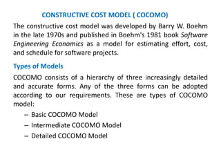
1. The constructive cost model was developed by Barry W. Boehm
in the late 1970s and published in Boehm's 1981 book Software
Engineering Economics as a model for estimating effort, cost,
and schedule for software projects.
Types of Models
COCOMO consists of a hierarchy of three increasingly detailed
and accurate forms. Any of the three forms can be adopted
according to our requirements. These are types of COCOMO
model:
– Basic COCOMO Model
– Intermediate COCOMO Model
– Detailed COCOMO Model
CONSTRUCTIVE COST MODEL ( COCOMO)
2. The constructive cost model was developed by Barry W. Boehm
in the late 1970s and published in Boehm's 1981 book Software
Engineering Economics as a model for estimating effort, cost,
and schedule for software projects.
Types of Models
COCOMO consists of a hierarchy of three increasingly detailed
and accurate forms. Any of the three forms can be adopted
according to our requirements. These are types of COCOMO
model:
– Basic COCOMO Model
– Intermediate COCOMO Model
– Detailed COCOMO Model
CONSTRUCTIVE COST MODEL ( COCOMO)
3. In COCOMO, projects are categorized into three types:
1. Organic
2. Semidetached
3. Embedded
1. Organic
If the project deals with developing a well-understood
application program, the size of the development team is
reasonably small, and the team members are experienced in
developing similar methods of projects.
Examples of this type of projects are simple business systems,
simple inventory management systems, and data processing
systems.
4. 2. Semidetached
If the development consists of a mixture of experienced and
inexperienced staff. Team members may have finite experience
in related systems but may be unfamiliar with some aspects of
the order being developed.
Example
Developing a new operating system (OS), a Database
Management System (DBMS), and complex inventory
management system.
3. Embedded
A software project with requiring the highest level of complexity,
creativity, and experience requirement fall under this category.
For Example: ATM, Air Traffic control.
Note - All the above system types utilize different values of the
constants used in Effort Calculations.
5. Calculations of Efforts & development time
1. Basic COCOMO Model:
The basic COCOMO model provide an accurate size of the project
parameters. The following expressions give the basic COCOMO
estimation model:
Effort = a1 x (KLOC) ^ a2 PM
Tdev = b1 x (Effort) ^ b2 Months
• Where
• KLOC is the estimated size of the software product indicate in
Kilo Lines of Code,
• a1,a2,b1,b2 are constants for each group of software products,
• Tdev is the estimated time to develop the software, expressed
in months,
• Effort is the total effort required to develop the software
product, expressed in person months (PMs).
6. Estimation of Development Effort
For the three classes of software products, the formulas for
estimating the effort based on the code size are shown below:
Organic: Effort = 2.4 (KLOC)^1.05 PM
Semi-detached: Effort = 3.0 (KLOC)^1.12 PM
Embedded: Effort = 3.6 (KLOC)^1.20 PM
Estimation of Development Time
For the three classes of software products, the formulas for
estimating the development time based on the effort are given
below:
Organic: T dev = 2.5 (Effort)^0.38 Months
Semi-detached: T dev = 2.5 (Effort)^0.35 Months
Embedded: T dev = 2.5 (Effort)^0.32 Months
7. Example1: Suppose a project was estimated to be 400 KLOC. Calculate
the effort and development time for each of the three model i.e.,
organic, semi-detached & embedded.
Solution: The basic COCOMO equation takes the form:
Effort=a1*(KLOC)^a2 PM
Tdev=b1*(efforts) ^b2 Months
Estimated Size of project= 400 KLOC
(i)Organic Mode
E = 2.4 * (400) ^1.05 = 1295.31 PM
TDev = 2.5 * (1295.31) ^ 0.38=38.07 PM
(ii)Semidetached Mode
E = 3.0 * (400)^1.12=2462.79 PM
TDev = 2.5 * (2462.79)^ 0.35=38.45 PM
(iii) Embedded Mode
E = 3.6 * (400)^1.20 = 4772.81 PM
TDev = 2.5 * (4772.8)^0.32 = 38 PM
8. 2. Intermediate COCOMO Model
The intermediate COCOMO model refines the initial estimates
obtained through the basic COCOMO model by using a set of 15
cost drivers based on various attributes of software engineering.
Classification of Cost Drivers and their attributes:
(i) Product attributes -
a. Required software reliability extent
b. Size of the application database
c. The complexity of the product
(ii) Hardware attributes -
a. Run-time performance constraints
b. Memory constraints
c. The volatility of the virtual machine environment
d. Required turnabout time
9. Intermediate COCOMO Contd…
(iii) Personnel attributes -
a. Analyst capability
b. Software engineering capability
c. Applications experience
d. Virtual machine experience
e. Programming language experience
(iv) Project attributes -
a. Use of software tools
b. Application of software engineering methods
c. Required development schedule
10. Intermediate Cocomo Contd…
Intermediate COCOMO equation:
E = ai (KLOC)^ bi*EAF
T Dev = ci (E)^di
Coefficient for Intermediate COCOMO
Project Ai Bi Ci Di
Organic 2.4 1.05 2.5 0.38
Semidetached 3.0 1.12 2.5 0.35
Embedded 3.6 1.20 2.5 0.32
11. 3. Detailed COCOMO Model
In detailed Cocomo, the whole software is differentiated into
multiple modules, and then we apply COCOMO in various
modules to estimate effort and then sum the effort.
The Six phases of detailed COCOMO are:
1. Planning and requirements
2. System structure
3. Complete structure
4. Module code and test
5. Integration and test
6. Cost Constructive model
12. Software Requirement Specification
A software requirements specification (SRS) is a detailed description of a software system
to be developed with its functional and non-functional requirements. The SRS is developed
based on the agreement between customer and developer. It may include the use cases of
how user is going to interact with software system.
Characteristics of a good SRS
1. Correctness
2. Modifiability
3. Completeness
4. Unambiguousness
5. Verifiability
6. Traceability
7. testability
8. Consistent
9. Design independence
10. Ranking for importance
11. Understandable by the customer
12. Right Level of abstraction
15. Parts of a SRS Document
1. Functional Requirements of the system
2. Non-functional Requirements of the system
3. Goals of implementation
16. Functional Requirements-
Functional requirements for a system describe what the system
should do. It describes the system functions like inputs, outputs,
exceptions and so on. It can be a calculation, data manipulation,
business process, user interaction, or any other specific
functionality which defines what function a system is likely to
perform.
Example- The software system should be integrated with banking
API
{ Fi}
INPUT OUTPUT
I1
I2
IN
O1
O2
ON
18. Entity Relationship (ER) – Data Model
It is a graphical representation of logical relationships of entities. It shows
that how various entities are related to each other in a database. An E-R
diagram represents the whole structure of a database. It shows what
entities are there in database, what attributes they are having and what
kind of relationships are there among entities.
Components of E-R Diagram (Graphical representation)
1. Entity -
2. Attribute –
3. Relationship -
4. Primary Key Attribute –
5. Multi-valued attribute -
19. Entity – It is real world object distinguishable from other objects. Each
entity has some properties which uniquely identify the entity.
Example-
1. Each employee of an organisation is an entity which has some properties
like employee id, employee name, designation, DOB, Basic Pay etc.
2. Each student of an Institute is an entity which has some properties like
student roll no, student name, branch, Dob etc.
Entity Set – The set of entities of same kind which share the same
properties or attributes.
Example – “EMPLOYEE” table is an entity set of all employees.
EMP_ID EMP_NAME DEPT DESG
1001 RAMESH CE LECTURER
1002 MANISH ECE ASSTT
1003 RAVEENA DE LECTURER
20. TYPES OF ENTITY
1. WEAK ENTITY - An entity which does not have sufficient attributes to
form a primary key is called a Weak-Entity. It is represented by double
ractangle
Example –
DEPARTURE – ENTITY CHILDREN - ENTITY
DEPARTURE
DEP_DATE CHILDREN
CNAME AGE
GENDER
21. 2. STRONG ENTITY -
The entity which has a primary key attribute is called as strong entity. It is
represented by a rectangle.
STUDENT
ROLL_NO NAME
GENDER
AGE
22. ATTRIBUTE
The property of an entity is called an attribute. Attributes are the
information about the entity which we want to store.
Example-
1. EMP_ID, EMP_NAME, DESG, DOB, DEPT, SALARY etc are the attributes
of “EMPLOYEE” entity.
2. STU_ID,NAME,AGE,GENDER etc are the attributes of “STUDENT” entity.
TYPES OF ATTRIBUTES
1. SIMPLE ATTRIBUTE – It is an attribute which can not be further divided.
Example – “SALARY” of a person is simple attribute because it can not be
further devided.
2. COMPOSITE ATTRIBUTE – Which can be further devided.
Example- “NAME” of a person can be further devided as “FIRST NAME”,
“MIDDLE NAME” and “LAST NAME”
3. SINGLE VALUED ATTRIBUTE- Which can have only single value.
Example – “GENDER” can have only one value either “MALE” or “FEMALE”
4. MULTI-VALUED ATTRIBUTE- Which can have more than one value.
Example – “CONTACT_NO” may have more than one value.
23. RELATIONSHIP
The association between entities is called relationship.
RELATIONSHIP SET - Set of relationships of same type.
CARDINALITY - The number of entities to which another entity can be
associated via a relationship set.
TYPES OF RELATIONSHIPS
1. ONE-TO-ONE ( 1 : 1 )
One record in Table-A is associated with only one record in Table-B.
1 Relationship 1
1 Relationship 1
1 Relationship 1
More Example- DRIVER – LICENSE, CITIZEN-AADHAR, PERSON-PASSPORT
DEPARTMENT_1 DEPT_1_HEAD
DEPARTMENT_2 DEPT_2_HEAD
DEPARTMENT_3 DEPT_3_HEAD
24. 2. ONE-TO-MANY (1 : M )
One record in Table-A (Parent Table) can be associated with any records in
Table-B (Child Table).
1 M
More example –
Department – Employee, Mother-Children, Student-Books,
FATHER CHILDREN
25. 3. MANY-TO-MANY RELATIONSHIP ( M : M)
One record in Table-A is associated with any number of records in Table-B
and one record in Table-B is associated with any number of records in
Table-A.
M M
More Example-
Book-Author, Course-Teacher, Course-Student
DOCTOR PATIENT
26. E-R DIAGRAM FOR LIBRARY MANAGEMENT SYSTEM
For drawing E-R diagram, the following database activities are to be
performed-
1. Identify all Objects (Entities about which information are to be stored.
2. Define attributes for each entity with a primary key for each entity.
3. Define relationships among entities.
ENTITIES
1. BOOK : (book_id, title, category, price)
2. STUDENT : (student_id,name,semester,contact_no, address, fine)
3. AUTHOR : (author_id, name, contact_no, address)
4. PUBLISHER : (pub_id, name, contact_no, address)
RELATIONSHIPS
BOOK : AUTHOR (M : M)
BOOK : STUDENT (M : M)
PUBLISHER : BOOK ( 1 : M)
27.
28. Data Flow Diagram
• A Data Flow Diagram (DFD) is a traditional visual
representation of the information flows within a system.
• It shows how data enters and leaves the system, what
changes the information, and where data is stored
• The DFD is also called as a data flow graph or bubble chart.
30. Levels in Data Flow Diagrams (DFD)
0-Level DFD
1-Level DFD
2-Level
0-Level DFD
It represents the entire software requirement as a single bubble
with input and output data denoted by incoming and outgoing
arrows. Then the system is decomposed and described as a DFD
with multiple bubbles.
32. 1-level DFD
In 1-level DFD, a context diagram is decomposed into multiple
bubbles/processes. In this level, we highlight the main objectives
of the system and breakdown the high-level process of 0-level
DFD into sub-processes.
34. 2-Level DFD
2-level DFD goes one process deeper into parts of 1-level DFD. It
can be used to project or record the specific/necessary detail
about the system's functioning.
40. Data Dictionary
A data dictionary contains metadata i.e data about the database.
It contains general information about the following −
Names of all the database tables and their schemas.
Details about all the tables in the database, such as their
owners, their security constraints, when they were created etc.
Physical information about the tables such as where they are
stored and how.
Table constraints such as primary key attributes, foreign key
information etc.
Information about the database views that are visible.
41. Data Dictionary- an example
Describing the Employee Details
Field Name Data Type Field Size for
display
Description Example
Employee
ID
Integer 10 Unique ID of
Employee
1001
Name Text 50 Name of
Employee
Ramesh
Date of Birth Date/Time 10 Date of Birth 10/01/1983
Phone Number Integer 10 Mobile
Number
9834343464
42. Types of Data Dictionary
Active Data Dictionary
When any changes are made in the database, the
data dictionary is automatically updated by the
database management system This is known as an
active data dictionary as it is self updating.
Passive Data Dictionary
When the database is modified, the database
dictionary is not automatically updated as in the
case of Active Data Dictionary.
A passive data dictionary is maintained separately
to the database whose contents are stored in the
dictionary.