2. 2146 J. Pringle et al.: Atmospheric circulation patterns and wave climates
attempts to model wave characteristics derived from circula-
tion patterns can be difficult and time-consuming. Statistical
knowledge gained from the observations of wave climates
and pressure fields allows insight into this complex relation-
ship without the need for explicit physical coupling. This can
be a useful tool for risk analysis since it provides insight into
the source of extreme events. If we understand the circulation
patterns that drive extreme events, then their occurrence (or
the occurrence of similar patterns) can have a degree of risk
attached to it. For example the risk could be the likelihood of
an extreme wave event, of severe erosion, of extended storm
durations, or a combination of all three.
Circulation patterns are herein described in terms of
pressure anomalies on the 700 hPa geopotential. The
types/classes or groups of anomalies can be specified by two
approaches: (1) those specified prior to classification and
(2) those that are derived and evolve during the classifica-
tion process (Huth et al., 2008). In the past, anomaly pat-
terns were identified by experts in the field: examples are
the Hess–Brezowsky catalogue or the Lamb classification
(Lamb, 1972; Hess and Brezowsky, 1952; Huth et al., 2008).
However the power of modern computers provides a means
to generate numerical solutions to complicated algorithms
that can automate the process.
It is important to note that atmospheric circulation pat-
terns are not a set of separated, well-defined states. CPs
change smoothly between states that form part of a con-
tinuous sequence of events (Huth et al., 2008). Therefore
the classes (or types) merely represent simplified climatic
events responsible for specific variables of interest. While
automated derivations of classification types utilize objec-
tive reasoning, according to Huth et al. (2008) the procedure
as a whole cannot be considered fully objective. A num-
ber of subjective decisions are still employed. For exam-
ple the number of CPs to use and the method of differen-
tiating classes. Existing objective-based classification algo-
rithms such as self-organizing maps (SOMs), principle com-
ponent analysis (PCA) and cluster analysis provide effective
ways to visualize the complex distribution of synoptic states
(Huth et al., 2008; Hewitson and Crane, 2002). These ap-
proaches are fundamentally based on only the predictor vari-
ables (atmospheric pressure anomalies in our case). Links to
surface weather variables are only made once the classifica-
tion technique has been carried out. This can therefore lead
to non-optimal links to the variable of interest (Bárdossy,
2010).
The classification method used for this study is a fuzzy-
rule-based algorithm developed by Bárdossy et al. (1995).
The classification technique aims to find strong links between
atmospheric CPs and a variable of interest, for this study the
wave height. The algorithm was originally used to link atmo-
spheric CPs with rainfall events (Bárdossy et al., 2002). In
the present study the method has been adapted to use wave
heights to guide the classification procedure. The main aim of
this paper is to investigate the feasibility of using this method
31°E 31.5°E 32°E
29.5°S
29°S
0 25 50
km
Durban Wave Rider
(29.9S,31.1E)
Richards Bay
Wave Rider
(28.8S,32.1E)
20°E 30°E
25°S
30°S
0 250500
km
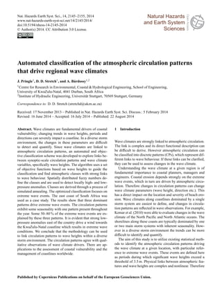
Figure 1. Locations of the wave observation buoys at Durban and
Richards Bay, along the KwaZulu-Natal coastline.
to identify CPs that are the main drivers of regional wave cli-
mates for application to coastal vulnerability assessments.
2 Methods
2.1 Case study site
The KwaZulu-Natal (KZN) coastline (Fig. 1) has a high-
energy wave climate. Tropical cyclones, mid-latitude (extra-
tropical) cyclones and cut-off lows have been cited as impor-
tant drivers of the local wave climate (Mather and Stretch,
2012; Corbella and Stretch, 2012b; Rossouw et al., 2011).
Tropical cyclones that become stationary to the south east
of Madagascar can occasionally drive large wave events that
cause severe beach erosion in KZN (Mather and Stretch,
2012; Corbella and Stretch, 2012b). Cut-off lows are deep
low-pressure systems that are displaced from the normal
path of west–east moving mid-latitude cyclones (Preston-
Whyte and Tyson, 1988). Instabilities within the westerly
zonal flow, due to the high wind shear, create vortices (and
low pressures) that can become cut-off and move equator-
ward (Preston-Whyte and Tyson, 1988). This diverse storm
environment leads to seasonality within the wave climate. On
average autumn and winter are associated with the largest
wave energy, while summer has the smallest (Corbella and
Stretch, 2012b). Seasons are defined according to Table 1.
2.2 Sources of data
Wave data were obtained from wave measurement buoys at
two locations along the KwaZulu-Natal coastline (Fig. 1)
for the period 1992–2009. A comparison of the wave data
from the Durban and Richards Bay measurement locations
by Corbella and Stretch (2012b) showed a strong correlation.
Nat. Hazards Earth Syst. Sci., 14, 2145–2155, 2014 www.nat-hazards-earth-syst-sci.net/14/2145/2014/
3. J. Pringle et al.: Atmospheric circulation patterns and wave climates 2147
Table 1. The allocation of months to seasons.
Season Months
Summer January–March
Autumn April–June
Winter July–September
Spring October–December
Therefore, where necessary, the two data sets were used to
fill in missing data to provide a continuous wave record for
the KwaZulu-Natal coastline. The data comprised significant
wave heights, maximum wave heights, wave periods, and
wave directions at 3-hourly intervals. However only daily
values of significant wave heights were used for the analy-
sis reported here.
The CP classification procedure was applied to daily nor-
malized pressure anomalies that describe atmospheric circu-
lation patterns. The anomalies were derived from the 700 hpa
geopotential height with a grid resolution of 2.5◦ (10◦ S,
0◦ E–50◦ S, 50◦ E). Geopotential heights were obtained from
the ERA-Interim data set for the period 1979–2009 (http:
//apps.ecmwf.int/datasets/). Letting k(i, t) be the geopoten-
tial height at location i and time t, then the anomaly at loca-
tion i and time t is defined as
h(i, t) =
k(i, t) − k(i)
σ(i)
, (1)
where k(i) and σ(i) are the average and standard deviation
of the geopotential at location i.
2.3 Classification methods
The classification used herein comprises two parts: (1) an
optimization procedure in which a set of classes defining at-
mospheric states are derived using an optimization process
as described in Sect. 2.4, and (2) a classification method that
involves a process of assigning CPs to the classes.
The aim is to identify a classification in which the set
of classes defining atmospheric pressure fields can explain
the occurrence of wave events at a specified location. There
are many ways in which classification algorithms can be
constructed. Classifications can be subjective, objective or
a mixture of both (Bárdossy, 2010; Huth et al., 2008). Ob-
jective classification algorithms employ a self-learning tech-
nique whereby atmospheric classes are derived through an
optimization procedure (for examples see Bárdossy, 2010;
Bárdossy et al., 2002; Huth et al., 2008; Hewitson and Crane,
2002). Since the goal is to gain insight into the drivers of a re-
gional wave climate, it follows that the wave climate should
be included within the optimization procedure (see Sect. 2.4).
Then the set of CP classes that are derived have strong links
to the regional wave climate. Furthermore, classes linked
with these variables explain, as best possible, their occur-
rences. This is a useful tool in guiding the algorithm to an
optimal solution. Classifying CPs linked to extreme wave
events is the focus of this study. The classifying procedure
uses wave heights as the dependent variable to find classes
of the independent variable, atmospheric pressure anoma-
lies. The method of classification is described in detail by
Bárdossy et al. (1995); Bárdossy et al. (2002) and Bárdossy
(2010). Only a brief overview is given here.
The classification method used herein is fuzzy-rule-based
which incorporates the use of fuzzy sets (Zadeh, 1965). This
allows the algorithm to handle imprecise statements such as
“strong high pressure” or “low pressure” (Bárdossy et al.,
1995). The CPs at each time realization are assigned to a cer-
tain CP class or group. Each CP class is defined by a rule
which comprises a number of fuzzy set membership func-
tions. The nth CP class is described by the fuzzy rule n as
a vector cn = [V (1, n), ..., V (i, n), ..., V (K, n)], for all
available grid points (1, ..., K), where V is the matrix con-
taining all CP rules and the index V (i, n) is the fuzzy set
number corresponding to the location i for rule n. The rules
consist of the following fuzzy sets:
1. fuzzy set number 0 – any type of anomaly,
2. fuzzy set number 1 – strong positive anomaly,
3. fuzzy set number 2 – weak positive anomaly,
4. fuzzy set number 3 – weak negative anomaly and
5. fuzzy set number 4 – strong negative anomaly.
The fuzzy set numbers (1, ..., 4) describe the locations of
different pressure types. However, the fuzzy set number 0 is
irrelevant for the CP classification. In general most of the
grid points belong to this fuzzy set number. The algorithm
only considers patterns with structures corresponding to the
arrangement of the fuzzy set numbers 1, ..., 4.
From the fuzzy set numbers described above, a member-
ship grade µ at location i can be assigned for each daily
anomaly pattern as
µn,j (i, t) = g (cn(i), t), (2)
where n is the fuzzy rule, g(cn(i), t) is the membership
function for the fuzzy set number j at location i at time t
(Bárdossy et al., 2002). The membership grade µ at each
location ranges between 0 and 1 based on the membership
function for the location specific fuzzy number. A value
of 0 implies that the anomaly value has no association with
the fuzzy number, and a value of 1 implies the anomaly is
strongly associated with the fuzzy number. It follows that a
combination of the membership grades provide insight into
the performance of each CP rule in relation to the daily
anomaly patterns. A degree of fit (DOF) is computed for each
CP rule, and the rule with the highest DOF value is assigned
to the circulation pattern class for that day. The degree of fit
is defined as follows (Bárdossy et al., 1995; Bárdossy et al.,
2002):
www.nat-hazards-earth-syst-sci.net/14/2145/2014/ Nat. Hazards Earth Syst. Sci., 14, 2145–2155, 2014
4. 2148 J. Pringle et al.: Atmospheric circulation patterns and wave climates
DOF(n, t) =
4
j=1
1
N(n, j)
N(n,j)
i=1
µn,j (i, t)Pj
1
Pj
, (3)
where t is the day, N(n, j) is the number of grid points cor-
responding to the fuzzy set number j for fuzzy rule n, the
term
N(n,j)
i=1
µn,j (i, t) sums all the membership grades at var-
ious locations corresponding to the fuzzy set number j for
rule n, and the exponent Pj is a parameter that allows us to
emphasize the influence of selected rules on the DOF.
The CP rules were obtained via an optimization proce-
dure following Bárdossy et al. (2002), which is described in
Sect. 2.4.
2.4 Optimization methods
The goal of the optimization is to derive a set of CP classes
or rules defining dominant circulation patterns in a partic-
ular region. The rules are strongly linked to a variable of
interest. The optimization procedure should maximize dis-
similarity between the CP types while minimizing the vari-
ability within the classes. The significant wave height (Hs)
was selected as the variable of interest for this study. The
algorithm considers both the daily average significant wave
height and the daily maximum significant wave height. The
optimization procedure was carried out for the period con-
taining all wave data (1992–2009). A simulated annealing
algorithm following Aarts and Korst (1989) is used in the
optimization procedure. Details of the process are given in
Bárdossy et al. (2002). The algorithm may be briefly outlined
as follows:
1. Randomly assigned CP rules are initialized and their
performance is evaluated through an objective func-
tion O.
2. The initial “annealing temperature” is set to q0.
3. A rule n is selected randomly.
4. A location i is selected randomly.
5. A fuzzy number c∗ is selected randomly.
6. If cn(i) = c∗, return to step 2.
7. Set cn(i) = c∗ and run the classification.
8. Calculate the new performance O∗ for the new rules.
9. If O∗ > O, accept the change.
10. If O∗ ≤ O, accept the change with probability
exp O −O∗
qj
.
11. If the change has been accepted, replace O by O∗.
12. Repeat steps 2–10 a specified number of iterations.
13. Decrease the “annealing temperature” such that
qnew < qold.
14. Repeat steps 2–12, until the number of accepted
changes becomes less than a predefined limit.
The optimization process relies strongly upon a set of ob-
jective functions. The objective functions are based on the
extreme wave events, wave heights and storm duration as dis-
cussed below.
Objective functions
A good classification contains classes with corresponding
wave statistics which differ from the statistics calculated
without classification. The goal of the classification is to ob-
tain a set of CP rules which correspond to the occurrence
of extreme waves. Extreme waves events are defined where
Hs ≥ 3.5 m. Therefore the objective functions used within the
algorithm are designed to optimize the CP occurrences which
coincide with extreme wave events. These are relatively rare
events. A random classification leads to the same probability
of occurrence as the mean for each rule, which is undesir-
able (Bárdossy, 2010). A good classification should lead to
rules that differ from the climatological mean for the selected
variable, in this case the wave height.
The intention of this classification is to find CPs that drive
extreme wave events. Three objective functions were used
as the performance measures. The first objective function re-
lates to the conditional probability of an event based on the
occurrence of a CP class. It is given as
O1(θ) =
T
t=1
hCP(t) (p(Hs ≥ θ|CP(t)) − p)2
, (4)
where θ is a predefined threshold, T is the total number of
days, hCP(t) is the frequency of the CP class, p(CP(t)) is the
probability that the threshold is exceeded for a given CP on
a day t, and p is the unclassified probability of exceedance
for all days in period T . The advantage of incorporating a
predefined threshold θ is to allow the algorithm to evaluate
different scenarios. For this study two different thresholds
were considered. The first relates to extreme wave events
where θ1 = 3.5 m. The second, with θ2 = 2.5 m, allows the
algorithm to explore a larger data set for deriving the classes.
Another useful measure of performance relates to the
mean significant wave heights. The ratio between the CP
class-averaged wave heights to the unclassified mean pro-
vides information on the separability of the classes from the
mean. Therefore the second objective function incorporating
average significant wave heights is defined as
O2 =
T
t=1
hCP(t)
Hs(CP(t))
Hs
− 1 , (5)
Nat. Hazards Earth Syst. Sci., 14, 2145–2155, 2014 www.nat-hazards-earth-syst-sci.net/14/2145/2014/
5. J. Pringle et al.: Atmospheric circulation patterns and wave climates 2149
where Hs(CP(t)) is the mean significant wave height on a
day with the given CP(t) class and Hs is the mean daily wave
height without classification. Storm durations are defined as
the times from when wave heights exceed 3.5 m to the time
when they again reduce below 3.5 m. To account for the per-
sistence of types of CPs during extreme events, Eq. (5) was
modified to include storm durations as
O3 =
T
t=1
hCP(t)
D(CP(t))
D
− 1 , (6)
where D(CP(t)) is the average storm duration for the CP(t)
class and D is the unclassified average storm duration.
A weighted linear combination of Eqs. (4), (5) and (6) was
used to optimize the solution to the classification algorithm.
The weights were chosen to emphasize the importance of cer-
tain objective functions relative to others and to correct for
the different magnitudes of the three objective functions.
2.5 Classification quality
Classification quality refers to the ability of the algorithm
to maximize dissimilarity between a set of CP classes while
minimizing variability within each CP class. This study
focuses on classifying CPs driving extreme wave events.
Therefore there are two criteria for measuring the classifi-
cation quality. The first is the ability of the classification to
explain extreme wave events. The second is the variability
of the classifications within each CP class. There exists an
optimal number of CP rules which successfully explain ex-
treme events and daily CP realizations. Too few rules implies
that the resulting CPs do not allow a proper distinction of
the causal mechanisms and would lead to classes which have
statistics similar to the unclassified case. Too many classes
increases the computational effort and captures features that
are not general and do not correspond to the wave generating
mechanisms. Bárdossy (2010) suggests utilizing the objec-
tive functions as a measure of the classification quality. Huth
et al. (2008) list a number of different quality measures that
explain the separability between and variability within CP
classes. For this study the variability within the classes as
well as the degree of fit are used as measures of the classi-
fication quality. This provides insight into the performance
of the classes with respect to their ability to explain average
CPs.
The variability of extreme events is defined as the position
of the lowest anomaly relative to the average pattern. This
was assumed as the storm centre. Wave events are driven by
storms associated with low pressures (i.e. negative anoma-
lies). The performance of the CP classes in explaining ex-
treme wave events can be measured by their relative con-
tribution to extreme events, namely p(CP|Hs ≥ θ), where θ
is a predefined threshold (for this study 3.5 m). A classifica-
tion strongly linked to the wave climate should define classes
whose frequency of occurrence corresponds to the average
and extreme wave events. This implies that CPs driving ex-
treme events should occur infrequently, whereas CPs driving
the average wave climate should occur more frequently.
3 Results
3.1 Dominant CP classes
The objective functions (Eqs. 4, 5 and 6) were used to de-
rive a set of CP classes which explain extreme wave events.
Figure 2 shows the average anomaly patterns for all the CP
classes. CP99 refers to an unclassified class. Useful statis-
tical parameters relevant to this study for a given CP class
are (a) frequency of occurrence, (b) percentage contribution
of extreme events, and (c) average and maximum significant
wave heights (Hs). These parameters are obtained from the
classification and are shown in Table 2.
The results show two trends in CPs that drive wave devel-
opment. Firstly CP01 and CP02 (Fig. 2a and b) according to
Table 2 occur most frequently (∼ 17 % of the time). CP01 re-
sembles that of mid-latitude cyclones which frequently travel
in a west to east direction south of the country, while CP02
resembles the high-pressure systems that follow the mid-
latitude cyclones. Secondly, Table 2 shows that CP03 is as-
sociated with 30–60% of all extreme wave events. The large
contribution by this class to extreme events is present all
year-round with the highest contribution in winter (∼ 65 %).
CP03 (Fig. 2c) occurs infrequently (7–9 % of the time), but
when it does occur it is associated with average and maxi-
mum significant wave heights ranging from 2.4 to 3.0 and
from 5.0 to 8.5 m, respectively. CP05 and CP06 (Fig. 2e
and f) according to the classification are responsible for about
30 % of extreme events in spring and summer, respectively.
CP06 represents low-pressure anomalies southeast of Mada-
gascar. This appears to resemble the strong low-pressure sys-
tems that are associated with tropical cyclones. According to
Mather and Stretch (2012) low-pressure systems southeast
of Madagascar can cause large swells. CP05 resembles low-
pressure systems over the interior which extend southwards.
No time lag was considered when deriving the CP classes.
This constrains the algorithm to only consider CPs occurring
on the day of a wave event and assumes that extreme events
are driven by relatively stationary CPs.
3.2 CP variability
3.2.1 Degree of fit (DOF)
The degree of fit relates to how well the CP for each day is
classified as a given class relative to the rule file. The larger
the degree of fit is, the stronger the relation between the CP
and the CP class. Figure 4 shows the average anomaly pat-
tern for CP03 together with the CPs associated with both the
highest and lowest degree of fit value for that class. CP03 is
associated with cut-off lows to the east/south-east of South
www.nat-hazards-earth-syst-sci.net/14/2145/2014/ Nat. Hazards Earth Syst. Sci., 14, 2145–2155, 2014
6. 2150 J. Pringle et al.: Atmospheric circulation patterns and wave climates
6 Pringle, Stretch & B´ardossy: Atmospheric circulation patterns & wave climates
0E 20E 40E
50S
30S
10S
Longitude
Lattitude
0.2
0.4
0.6
0.8
−0.8
−0.6
−0.4
−0.2
0E 20E 40E
50S
30S
10S
Longitude
Lattitude
0.2 0.4
0.6
0.8
−0.6
−0.4
−0.2
−0.2
(a) CP01 (b) CP02
0E 20E 40E
50S
30S
10S
Longitude
Lattitude
0.8
0.6
0.4
0.2
−0.2
−0.4
−0.6
−0.8
0E 20E 40E
50S
30S
10S
Longitude
Lattitude
0.2
0.4
0.6
0.8
0.2
−0.4
−0.2
(c) CP03 (d) CP04
0E 20E 40E
50S
30S
10S
Longitude
Lattitude
0.2
0.4
0.6
0.8
0.2
−0.2
−0.4
−0.6
−0.8
0E 20E 40E
50S
30S
10S
Longitude
Lattitude
0.2
0.8
0.6
0.4
−0.2
−0.4
−0.6
−0.8
(e) CP05 (f) CP06
0E 20E 40E
50S
30S
10S
Longitude
Lattitude
0.8
0.6
0.4
0.2
−0.2
−0.4
−0.6
−0.8
0E 20E 40E
50S
30S
10S
Longitude
Lattitude
0.2
0.40.6
0.8
−0.8
−0.6
−0.4
−0.2
(g) CP07 (h) CP08
Fig. 2. Average anomaly patterns for all CP classes:1–8. Positive anomaly contours are shown as the dashed line while negative contours are
solid.
Figure 2. Average anomaly patterns for all CP classes: 1–8. Positive anomaly contours are shown as the dashed line while negative contours
are solid.
Nat. Hazards Earth Syst. Sci., 14, 2145–2155, 2014 www.nat-hazards-earth-syst-sci.net/14/2145/2014/
7. J. Pringle et al.: Atmospheric circulation patterns and wave climates 2151
Table 2. CP occurrence frequencies and wave height statistics associated with each CP. Statistics were calculated for the period 1992–2009.
Statistics CP01 CP02 CP03 CP04 CP05 CP06 CP07 CP08 CP99∗
Occurrence frequency (p(CP) %)
Summer 18 18 8.0 13 7.5 8.1 5.6 15 8.3
Autumn 18 19 8.0 11 10 7.2 5.1 13 8.8
Winter 16 17 8.1 12 11 8.4 4.5 14 8.9
Spring 17 16 9.1 12 9.4 7.7 5.0 15 9.2
All seasons 17 17 8.3 12 9.6 7.8 5.1 14 8.8
Threshold exceedance for a given CP (p(Hs ≥ θ|CP) %)
Summer – 0.4 8.0 0.3 – 3.5 2.6 0.7 –
Autumn 1.2 1.5 12 1.6 2.1 2.0 5.6 0.6 5.0
Winter 0.9 0.8 14 – 0.9 0.4 2.3 0.8 0.4
Spring 0.3 – 4.6 0.6 2.2 – 0.7 – –
All seasons 0.6 0.7 9.6 0.6 1.4 1.5 2.8 0.5 1.4
Exceedance contribution (p(CP|Hs ≥ θ) %)
Summer – 5.6 50 2.8 – 22 11 8.3 –
Autumn 7.7 10 33 6.4 7.7 5.1 10 2.6 17
Winter 7.5 7.5 64 – 5.7 1.9 5.7 5.7 1.9
Spring 4.5 – 55 9.1 27 – 4.5 – –
All seasons 5.8 7.4 48 4.2 7.9 6.9 8.5 4.2 7.4
Average Hs (m) for each CP
Summer 1.8 1.9 2.5 1.8 1.8 2.2 2.2 1.9 1.9
Autumn 1.8 1.9 2.7 1.9 2.0 2.0 2.1 1.9 2.1
Winter 2.0 2.0 2.9 1.9 2.1 2.0 2.2 2.0 1.9
Spring 2.0 1.9 2.4 1.9 2.2 2.0 2.2 2.0 2.0
All seasons 1.9 1.9 2.6 1.9 2.1 2.1 2.2 2.0 2.0
Standard deviation of Hs (m) for each CP
Summer 0.48 0.49 1.1 0.49 0.53 0.76 0.74 0.61 0.49
Autumn 0.58 0.66 1.0 0.70 0.76 0.66 0.90 0.55 1.0
Winter 0.58 0.61 0.94 0.55 0.66 0.58 0.66 0.55 0.67
Spring 0.51 0.49 0.84 0.52 0.71 0.50 0.61 0.50 0.49
All seasons 0.54 0.57 1.0 0.56 0.69 0.63 0.74 0.56 0.70
Max Hs (m) for each CP
Summer 3.4 4.0 8.5 3.7 3.4 5.0 5.2 5.6 3.3
Autumn 4.0 5.5 5.7 5.5 6.3 4.3 5.1 4.0 5.4
Winter 4.2 3.8 5.6 3.4 3.8 3.5 4.3 4.8 3.6
Spring 3.9 3.3 5.3 4.5 5.4 3.4 3.7 3.5 3.3
All seasons 4.2 5.5 8.5 5.5 6.3 5.0 5.2 5.6 5.4
∗ CP99 is the unclassified class. Blank entries imply zero occurrences in the data set.
Africa. The pattern also shows a strong high-pressure region
to the southwest. The combination of strong cut-off lows oc-
curring in conjunction with high-pressure regions comprises
an important feature for channelling waves towards the east-
ern coastline. Figure 4c is the CP with the lowest degree of
fit for the class CP03, and it shows only a weak anomaly
pattern.
3.2.2 Variability within classes
It is expected that in the vicinity of the regions defining rule
types (high or low pressures) the standard deviation should
be low. This is because the classification is based on the loca-
tion of these rules in comparison to the anomaly patterns for
specific days. Whereas the locations of “any anomaly” rule
types (fuzzy number 0) are expected to have significant vari-
ability, the variability in the vicinity of negative anomalies
www.nat-hazards-earth-syst-sci.net/14/2145/2014/ Nat. Hazards Earth Syst. Sci., 14, 2145–2155, 2014
8. 2152 J. Pringle et al.: Atmospheric circulation patterns and wave climatesPringle, Stretch & B´ardossy: Atmospheric circulation patterns & wave climates 9
0E 20E 40E
50S
30S
10S
Longitude
(a)
Lattitude
−1
−0.5
0
0.5
1
0E 20E 40E
50S
30S
10S
(b)
−4
−2
0
2
0E 20E 40E
50S
30S
10S
(c)
−2
−1
0
1
2
Fig. 3. (a) Average CP03 with (+) symbols indicating the centers of all negative anomalies (low pressures) contributing to the class. (b) &
(c) show actual CP’s for the dates 19/03/2007 and 30/08/2006 respectively, both of which were classified as members of the CP03 class.
0E 20E 40E
50S
30S
10S
Longitude
(a)
Lattitude
−1
−0.5
0
0.5
1
0E 20E 40E
50S
30S
10S
(b)
−3
−2
−1
0
1
0E 20E 40E
50S
30S
10S
(c)
0
0.5
1
1.5
2
0E 20E 40E
50S
30S
10S
Longitude
Lattitude
0.5
0.6
0.7
0.8
1
0.9
(d)
Fig. 4. Average anomaly pattern for CP03 (a) with (b) the anomaly
with highest DOF, (c) the anomaly with lowest DOF value, while
(d) shows the standard deviation for all CP03 anomalies.
Acknowledgements. Wave data for the study were provided by
eThekwini Municipality, Council for Scientific and Industrial Re-
search, and the SA National Port Authority. The ERA-Interim data555
were provided by ECMWF. We are grateful for funding from the
eThekwini Municipality, the National Research Foundation, and the
Nelson Endowment Fund in the UKZN School of Engineering.
References
Aarts, E. and Korst, J.: Simulated annealing and boltzmann ma-560
chines: a stochastic approach to combinatorial optimization and
neural computing., John Wiley & Sons, Chichester, 1989.
B´ardossy, A.: Atmospheric circulation pattern classification for
South-West Germany using hydrological variables, Physics and
Chemistry of the Earth, pp. 498–506, 2010.565
B´ardossy, A., Duckstein, L., and Bogardi, I.: Fuzzy rule-based clas-
sification of atmospheric circulation patterns, International Jour-
nal of Climatology, 15, 1087–1097, 1995.
B´ardossy, A., Stehlik, J., and Caspary, H. J.: Automated objective
classification of daily circulation patterns for precipitation and570
temperature downscaling based on optimized fuzzy rules., Cli-
mate Research, 23, 11–22, 2002.
Callaghan, D. P., Nielson, P., Short, A., and Ranasinghe, R.: Sta-
tistical simulation of wave climate and extreme beach erosion,
Coastal Engineering, 55, 375–390, 2008.575
Corbella, S. and Stretch, D. D.: Shoreline recovery from storms on
the east coast of South Africa, Natural Hazards and Earth System
Sciences, 12, 11–22, 2012a.
Corbella, S. and Stretch, D. D.: The wave climate on the the
KwaZulu Natal Coast, Journal of the South African Institute of580
Civil Engineering, 54, 45–54, 2012b.
Corbella, S. and Stretch, D. D.: Simulating a multivariate sea storm
using Archimedean copulas, Coastal Engineering, 76, 68–78,
2013.
Hess, P. and Brezowsky, H.: Katalog der Großwetterlagen Europas,585
Ber. DT. Wetterd. in der US-Zone 33, Bad Kissingen, Germany,
1952.
Hewitson, B. and Crane, R.: Self-organizing maps: applications to
synoptic climatology, Climate Research, 22, 13–26, 2002.
Figure 3. (a) Average CP03 with (+) symbols indicating the centres of all negative anomalies (low pressures) contributing to the class during
extreme events. (b) and (c) show actual CPs for the dates 19 March 2007 and 30 August 2006, respectively, both of which were classified as
members of the CP03 class.
0E 20E 40E
50S
30S
Longitude
(a)
Latti
−1
−0.5
0
5
3
1
Fig. 3. (a) Average CP03 with (+) symbols indicating the centers of all negative anoma
(c) show actual CP’s for the dates 19/03/2007 and 30/08/2006 respectively, both of whic
0E 20E 40E
50S
30S
10S
Longitude
(a)
Lattitude
−1
−0.5
0
0.5
1
0E 20E 40E
50S
30S
10S
(b)
−3
−2
−1
0
1
0E 20E 40E
50S
30S
10S
(c)
0
0.5
1
1.5
2
0E 20E 40E
50S
30S
10S
Longitude
Lattitude
0.5
0.6
0.7
0.8
1
0.9
(d)
Fig. 4. Average anomaly pattern for CP03 (a) with (b) the anomaly
with highest DOF, (c) the anomaly with lowest DOF value, while
(d) shows the standard deviation for all CP03 anomalies.
Acknowledgements. Wave data for the study were provided by
eThekwini Municipality, Council for Scientific and Industrial Re-
References
Aarts, E. and K560
chines: a sto
neural compu
B´ardossy, A.:
South-West G
Chemistry of565
B´ardossy, A., D
sification of
nal of Clima
B´ardossy, A., S
classification570
temperature
mate Researc
Callaghan, D. P
tistical simul
Coastal Engi575
Corbella, S. and
the east coast
Sciences, 12
Corbella, S. an
KwaZulu Na580
Civil Engine
Corbella, S. and
using Archim
2013.
Hess, P. and Bre585
Figure 4. Average anomaly pattern for CP03 (a) with (b) the anomaly with highest DOF, (c) the anomaly with lowest DOF value, while
(d) shows the standard deviation for all CP03 anomalies.
(low pressures) can be attributed to the movement of the low-
pressure systems. It is also expected that high-pressure sys-
tems are more stable with lower variability in their positions.
For example Fig. 4d shows lower variability in the vicinity
of the high-pressure region while high variability (standard
deviation of (1) in the low-pressure region. This can be at-
tributed to the movement of low-pressure systems around the
negative anomaly. Figure 4d shows high standard deviation
values in comparison to the mean negative anomaly. This
Nat. Hazards Earth Syst. Sci., 14, 2145–2155, 2014 www.nat-hazards-earth-syst-sci.net/14/2145/2014/
9. J. Pringle et al.: Atmospheric circulation patterns and wave climates 2153
could also indicate that CP anomalies driving extreme events
(cut-off lows) are associated with strong negative anomalies.
3.3 CP rules and extreme events
Daily CPs classified as in a certain class for extreme wave
events (Hs ≥ 3.5 m) were compared to the average patterns
for that class. Figure 3 shows the average pattern for CP03 to-
gether with selected extreme events corresponding to CP03.
The centres of the CPs are shown as “+” symbols in the
plot. A centre is defined as the location of the peak neg-
ative anomaly. The variability within the class is apparent.
However the majority of CPs classified as CP03 resemble
strong cut-off lows to the east/southeast of the country. It is
apparent that these strong cut-off lows drive extreme wave
events. Figure 5 and Table 3 show CPs associated with the
six largest significant wave height events. Four out the six
events have been classified as CP03, the class contributing to
the majority of extreme events. The concept of CPs belong-
ing, to some degree, to all the classes is evident in Fig. 5f.
This shows a similar pattern to CP04 and CP08, which both
represent low pressures southeast of Madagascar. However
according to the classification this CP belongs to class CP08
and not CP04. From visual inspection it appears to resemble
class CP04 better than CP08. Figure 5a and c are the CPs
associated with the March 2007 storm which caused severe
coastal erosion along the KwaZulu-Natal coastline (Mather
and Stretch, 2012; Corbella and Stretch, 2012a) with signifi-
cant wave heights reaching 8.5 m.
4 Discussion
Classifying circulation patterns is a useful tool for investi-
gating the occurrence of certain patterns over a given region.
There are many different techniques used for classifying CPs,
each of which has its benefits and drawbacks (Huth et al.,
2008). Classification can be subjective or objective (to a de-
gree). However the goal is always to group similar patterns
into individual classes. A useful application for engineering
purposes is utilizing a variable of interest to “guide” the al-
gorithm to find CPs linked to its occurrence. Bárdossy et al.
(2002) successfully implemented this to classify CPs that ex-
plained wet and dry events in Europe.
The emphasis of the present study has been on the sta-
tistical link between atmospheric circulation patterns and ex-
treme wave events. This is the first time the method described
here has been used in this context, and it has the potential
to improve current methods of risk analysis. The benefit of
fuzzy logic as a classification tool is that each daily CP be-
longs, to some degree, to all the CP classes. This is character-
istic of atmospheric circulation where daily CPs form part of
a continuum rather than a set of individual states as suggested
by the derived CP classes (Huth et al., 2008). However a po-
tential drawback of the method is the manner in which the
Table 3. Six of the most extreme wave events on record and their
associated CPs for the period 1992 to 2009.
Fig. 5 Date CP Hs (m)
(a) 19 Mar 2007 CP03 8.50
(b) 5 May 2001 CP05 6.30
(c) 18 Mar 2001 CP03 5.92
(d) 3 Apr 2001 CP03 5.66
(e) 23 Sep 1993 CP03 5.64
(f) 19 Mar 2001 CP08 5.63
CPs on each day are assigned to a class (Huth et al., 2008).
The degree of fit (Sect. 3) used in this study incorporates the
connectivity to a given class through and/or combinations of
high/low and not high/not low anomalies as described in Bár-
dossy et al. (1995). However this technique has been success-
ful in associating CPs with rainfall events (e.g. Bárdossy et
al., 2002; Bárdossy, 2010)
In the context of our case study site on the east coast
of South Africa, the most frequent CPs are low- and high-
pressure anomalies located south of the country. This can
be attributed to the west–east progression of mid-latitude
cyclones which frequent this area. They are major contrib-
utors to the wave climate along the South African coast-
line (Rossouw et al., 2011). The low-pressure systems can
become isolated after being displaced towards the Equa-
tor and can become stationary (Preston-Whyte and Tyson,
1988). These stationary cut-off lows can drive the devel-
opment of extreme wave events. Table 2 indicates that the
dominant CP that drives extreme events along the KwaZulu-
Natal coastline is CP03, which is associated with abnormally
low pressure to the east-southeast. CPs classified as CP03
resemble cut-off lows, and the pattern agrees with specula-
tions by Mather and Stretch (2012), Rossouw et al. (2011)
and Corbella and Stretch (2012b) concerning drivers of ex-
treme waves. Low-pressure anomalies linked to storms east
to south-east of South Africa drive wind fields that direct the
wave attack toward the coastline.
Callaghan et al. (2008) and Corbella and Stretch (2013)
highlight the importance of identifying independent storms
for risk analysis of extreme wave events. One limitation with
the methods described herein is that it is difficult to evaluate
the independence of the different CPs. A particular storm in
various stages of development may belong to a number of
CP classes rather than a single class according to the classi-
fication scheme. Examples are cut-off lows that become de-
tached from extratropical cyclones travelling west to east in
the region south of the country. The process of storm devel-
opment drives wave development. This suggests that it may
be better to locate a specific type of CP at any location rather
than a specified type of CP at a fixed location.
www.nat-hazards-earth-syst-sci.net/14/2145/2014/ Nat. Hazards Earth Syst. Sci., 14, 2145–2155, 2014
10. 2154 J. Pringle et al.: Atmospheric circulation patterns and wave climates10 Pringle, Stretch & B´ardossy: Atmospheric circulation patterns & wave climates
0 20 40
−50
−30
−10
19/3/2007− CP03
(a)
0 20 40
−50
−30
−10
5/5/2001− CP05
(b)
0 20 40
−50
−30
−10
18/3/2001− CP03
(c)
0 20 40
−50
−30
−10
3/4/2001− CP03
(d)
0 20 40
−50
−30
−10
23/9/1993− CP03
(e)
0 20 40
−50
−30
−10
19/3/2001− CP08
(f)
−3
−2
−1
0
1
2
3
Fig. 5. CP’s associated with the six largest significant wave heights for the dates (a) 19/3/2007, (b) 5/5/2001, (c) 18/3/2001, (d) 3/4/2001, (e)
23/9/1993 and (f) 19/3/2001.
Huth, R., Beck, C., Philipp, A., Demuzere, M., Ustrnul, Z.,590
Cahynov´a, M., Kysel´y, J., and Tveito, O. E.: Classifications of at-
mospheric circulation patterns: recent advances and application,
Annals of the New York academy of sciences, 1146, 105–152,
2008.
Komar, P. D., Allan, J. C., and Ruggiero, P.: Ocean Wave Cli-595
mates: Trends Variations Due to Earth’s Changing Climate, in:
Handbook of coastal and ocean engineering, edited by Kim, Y.,
chap. 35, pp. 972–995, World Scientific Publishing Co., Hacken-
sack, USA, 2010.
Lamb, H. H.: British Isles weather types and a register of the daily600
sequence of circulation patterns, 1861–1971, Meteorological Of-
fice, Geophysical Memoir No. 116, London: HMSO, 1972.
Mather, A. A. and Stretch, D. D.: A perspective on sea level rise
and coastal storm surge from southern and eastern Africa: a case
study near Durban, South Africa, Water, 4, 237–259, 2012.605
Preston-Whyte, R. A. and Tyson, P. D.: The atmosphere and weather
of Southern Africa, Oxford University Press, Cape Town, 1988.
Rossouw, J., Coetzee, L., and Visser, C.: A South African wave cli-
mate study, in: IPCC, 18, pp. 87–107, 1982.
Taljaard, J.: Development, Distribution and Movement of Cyclones610
and AntiCyclones in the South Hemishpere During the IGY,
Journal of Applied Meteorology, 6, 973–987, 1967.
Zadeh, L.: Fuzzy Sets, information control, 8, 338–353, 1965.
Figure 5. CPs associated with the six largest significant wave heights for the dates (a) 19 March 2007, (b) 5 May 2001, (c) 18 March 2001,
(d) 3 April 2001, (e) 23 September 1993 and (f) 19 March 2001.
5 Conclusions
A fuzzy-rule-based classification method has been adapted
to identify the atmospheric circulation patterns that drive re-
gional wave climates. The east coast of South Africa was
used as a case study. The method is based on normalized
anomalies in daily 700 hPa geopotential heights. The CP
classes are derived from an optimization procedure which is
guided by a variable of interest, in this case wave heights. The
classification shows a strong anomaly pattern east-southeast
of South Africa which explains 30–60 % of extreme wave
events. This CP type explains extreme events in all seasons.
However it occurs infrequently (∼ 8 % of the time) and is as-
sociated with large wave heights ranging from 5.0 to 8.5 m.
Frequently occurring CP classes have a similar structure to
mid-latitude cyclones or translational low-pressure systems
(followed by a zone of high pressure) that occur south of
South Africa (Taljaard, 1967).
The methodology discussed here appears to be new in the
context of wave climate analysis and has potential for appli-
cation to risk assessment studies in coastal management and
engineering.
Acknowledgements. Wave data for the study were provided by
eThekwini Municipality, Council for Scientific and Industrial
Research, and the SA National Port Authority. The ERA-Interim
data were provided by ECMWF. We are grateful for funding from
the eThekwini Municipality, the National Research Foundation, and
the Nelson Endowment Fund in the UKZN School of Engineering.
Edited by: R. Lasaponara
Reviewed by: three anonymous referees
References
Aarts, E. and Korst, J.: Simulated annealing and Boltzmann ma-
chines: a stochastic approach to combinatorial optimization and
neural computing, John Wiley & Sons, Chichester, 1989.
Bárdossy, A.: Atmospheric circulation pattern classification for
South-West Germany using hydrological variables, Phys. Chem.
Earth, 35, 498–506, 2010.
Bárdossy, A., Duckstein, L., and Bogardi, I.: Fuzzy rule-based clas-
sification of atmospheric circulation patterns, Int. J. Climatol.,
15, 1087–1097, 1995.
Bárdossy, A., Stehlik, J., and Caspary, H. J.: Automated objective
classification of daily circulation patterns for precipitation and
temperature downscaling based on optimized fuzzy rules, Clim.
Res., 23, 11–22, 2002.
Callaghan, D. P., Nielson, P., Short, A., and Ranasinghe, R.: Sta-
tistical simulation of wave climate and extreme beach erosion,
Coast. Eng., 55, 375–390, 2008.
Nat. Hazards Earth Syst. Sci., 14, 2145–2155, 2014 www.nat-hazards-earth-syst-sci.net/14/2145/2014/
11. J. Pringle et al.: Atmospheric circulation patterns and wave climates 2155
Corbella, S. and Stretch, D. D.: Shoreline recovery from storms on
the east coast of Southern Africa, Nat. Hazards Earth Syst. Sci.,
12, 11–22, doi:10.5194/nhess-12-11-2012, 2012a.
Corbella, S. and Stretch, D. D.: The wave climate on the the
KwaZulu Natal Coast, J. S. Afr. Inst. Civ. Eng., 54, 45–54, 2012b.
Corbella, S. and Stretch, D. D.: Simulating a multivariate sea storm
using Archimedean copulas, Coast. Eng., 76, 68–78, 2013.
Hess, P. and Brezowsky, H.: Katalog der Großwetterlagen Europas,
Ber. DT. Wetterd. in der US-Zone 33, Bad Kissingen, Germany,
1952.
Hewitson, B. and Crane, R.: Self-organizing maps: applications to
synoptic climatology, Clim. Res., 22, 13–26, 2002.
Huth, R., Beck, C., Philipp, A., Demuzere, M., Ustrnul, Z.,
Cahynová, M., Kyselý, J., and Tveito, O. E.: Classifications of at-
mospheric circulation patterns: recent advances and application,
Ann. New York Acad. Sci., 1146, 105–152, 2008.
Komar, P. D., Allan, J. C., and Ruggiero, P.: Ocean Wave Cli-
mates: Trends Variations Due to Earth’s Changing Climate, in:
Handbook of coastal and ocean engineering, edited by: Kim, Y.,
chap. 35, World Scientific Publishing Co., Hackensack, USA,
972–995, 2010.
Lamb, H. H.: British Isles weather types and a register of the daily
sequence of circulation patterns, 1861–1971, Geophysical Mem-
oir No. 116, Meteorological Office, HMSO, London, 1972.
Mather, A. A. and Stretch, D. D.: A perspective on sea level rise
and coastal storm surge from southern and eastern Africa: a case
study near Durban, South Africa, Water, 4, 237–259, 2012.
Preston-Whyte, R. A. and Tyson, P. D.: The atmosphere and weather
of Southern Africa, Oxford University Press, Cape Town, 1988.
Rossouw, J., Coetzee, L., and Visser, C.: A South African wave
climate study, Coastal Engineering Proceedings, 18, https://
journals.tdl.org/icce/index.php/icce/article/view/3618/3300 (last
access: August 2013), 2011.
Taljaard, J.: Development, Distribution and Movement of Cyclones
and AntiCyclones in the South Hemishpere During the IGY, J.
Appl. Meteorol., 6, 973–987, 1967.
Zadeh, L.: Fuzzy Sets, Information Control, 8, 338–353, 1965.
www.nat-hazards-earth-syst-sci.net/14/2145/2014/ Nat. Hazards Earth Syst. Sci., 14, 2145–2155, 2014