Projection of a Vector upon a Plane from an Arbitrary Angle, via Geometric (Clifford) Algebra
•
1 gefällt mir•591 views

We show how to calculate the projection of a vector, from an arbitrary direction, upon a given plane whose orientation is characterized by its normal vector, and by a bivector to which the plane is parallel. The resulting solutions are tested by means of an interactive GeoGebra construction.

Empfohlen
Empfohlen
Weitere ähnliche Inhalte
Was ist angesagt?
Was ist angesagt? (20)
Ähnlich wie Projection of a Vector upon a Plane from an Arbitrary Angle, via Geometric (Clifford) Algebra
Ähnlich wie Projection of a Vector upon a Plane from an Arbitrary Angle, via Geometric (Clifford) Algebra (20)
Mehr von James Smith
Mehr von James Smith (19)
Kürzlich hochgeladen
Kürzlich hochgeladen (20)
Projection of a Vector upon a Plane from an Arbitrary Angle, via Geometric (Clifford) Algebra
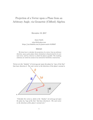
- 1. Projection of a Vector upon a Plane from an Arbitrary Angle, via Geometric (Clifford) Algebra December 19, 2017 James Smith nitac14b@yahoo.com https://mx.linkedin.com/in/james-smith-1b195047 Abstract We show how to calculate the projection of a vector, from an arbitrary direction, upon a given plane whose orientation is characterized by its nor- mal vector, and by a bivector to which the plane is parallel. The resulting solutions are tested by means of an interactive GeoGebra construction. Vector s is the “shadow” of vector g cast upon the plane by “rays of the Sun” that have direction ˆr. The unit vector in the direction of the plane’s normal is ˆe. “Calculate the vector s, which is the “shadow” of vector g cast upon the plane by “rays of the Sun” that have direction ˆr. The unit vector in the direction of the plane’s normal is ˆe.” 1
- 2. Contents 1 Introduction 2 2 Formulating the Problem in Geometric-Algebra (GA) Terms, and Devising a Solution Strategy 3 2.1 Initial Observations . . . . . . . . . . . . . . . . . . . . . . . . . . 3 2.2 Recalling What We’ve Learned from Solving Similar Problems Via GA . . . . . . . . . . . . . . . . . . . . . . . . . . . . . . . . 3 2.3 Further Observations, and Identifying a Strategy . . . . . . . . . 4 3 Solutions for s 4 3.1 Solution via the Inner Product with ˆe . . . . . . . . . . . . . . . 5 3.2 Solution via the Outer Product with T . . . . . . . . . . . . . . . 5 4 Testing the Formulas that We’ve Derived 7 5 Appendix: Calculating the Bivector of a Plane Whose Normal is the Vector ˆe 8 1 Introduction In this document, we will solve—numerically as well as symbolically—a problem of a type that can take the following concrete form, with reference to Fig.1: “A pole (not necessarily vertical) casts a shadow onto the perfectly flat plaza into which it is set. With respect to a right-handed orthonormal reference frame with basis vectors ˆa, ˆb, and ˆc, the direction of the Sun’s rays is ˆr = ˆara + ˆbrb + ˆcrc. The vector g from the pole’s base to the pole’s tip, is g = ˆaga + ˆbgb + ˆcgc, and the upward-pointing unit vector normal to the plane is ˆe = ˆaea+ˆbeb+ˆcec. Calculate s, the vector from the base of the pole to the tip of the pole’s shadow.”
- 3. Figure 1: Vector s is the “shadow” of vector g cast upon the plane by “rays of the Sun” that have direction ˆr. The unit vector in the direction of the plane’s normal is ˆe. 2 Formulating the Problem in Geometric-Algebra (GA) Terms, and Devising a Solution Strategy 2.1 Initial Observations Let’s begin by making a few observations that might be useful: 1. By saying “the direction of the Sun’s rays is ˆr = ˆara + ˆbrb + ˆcrc”, we assumed that all of the Sun’s rays are parallel. We’ll use that assumption throughout this document. 2. The tip of the shadow is at the point where a ray that just grazes the tip of the pole intersects the surface of the plaza. 3. Therefore, the vector from the tip of the pole to the tip of the shadow is some scalar multiple of ˆr. We’ll call that scalar multiple λˆr, and add it to our earlier diagram to produce Fig. 2. 4. From Fig. 2, we can see that s = g + λˆr. 2.2 Recalling What We’ve Learned from Solving Similar Problems Via GA Let’s also refresh our memory about techniques that we may have used to solve other problems via GA: 1. Problems involving projections onto a plane are usually solved by using the appropriately-oriented bivector that is parallel to the plane, rather than 3
- 4. Figure 2: The same situation as in Fig. 1, but noting that the vector from the tip of g to the tip of s is a scalar multiple (“λ”) of ˆr. by using the vector that is perpendicular to it. The Appendix (Section 5) shows how to find the required bivector, given said vector. 2. In a GA equation with two unknowns, such as the equation s = g + λˆr at the end of the preceding list, a common strategy is to eliminate one of the unknowns by using either the “dot” product or the ‘wedge” product (“∧”) with a known quantity. Examples of this strategy are given in Ref. [2], and in Ref. [3], pp. 39-47. 2.3 Further Observations, and Identifying a Strategy Guided by Sections 2.1 and 2.2, we might realize that the vector s is perpendicular to ˆe. Thus, one method of solving the equation s = g + λˆr is to eliminate s by “dotting” both sides with ˆe, thereby obtaining an equation that from which we can obtain an expression for λ in terms of g, ˆe, and ˆr. That expression can then be substituted for λ in the original eqation (s = g + λˆr) to find s. The same observations that led us to the first strategy also lead us to see that s is parallel to the plane of the plaza. Therefore, s’s product “∧” with the bivector that’s parallel to that plane is zero. That is, if we denote said bivector by the symbol “T”, then s ∧ T = 0. Using this observation, we also arrive at an equation for λ—and thus for s—but this time in terms of g, ˆr, and T. We’ll use both approaches in this document. 3 Solutions for s We’ll begin with the solution that uses the normal vector ˆe. 4
- 5. 3.1 Solution via the Inner Product with ˆe Taking up the first of the solution strategies that we identified in Section 2.3, we write s = g + λˆr; s · ˆe =0 = (g + λˆr) · ˆe; ∴ λ = − g · ˆe ˆr · ˆe . (3.1) Question: Does our expression for λ make sense? Let’s pause for a moment to examine that result before proceeding. Does it make sense? The geometric interpretation of that result is that |λ| is the ratio of the lengths of the projections of g and ˆr upon ˆe. So far, so good—a study of Fig. 2 confirms that |λ| must indeed be equal to that ratio. Examining Fig. 2 further, we see (1) that no shadow will be produced unless λ is positive, and (2) that no shadow will be produced unless the projections of g and ˆr are oppositely directed. Eq. (3.1) is consistent with those observations: λ is positive only when g · ˆe and ˆr · ˆe are opposite in sign, and that difference in sign occurs only when ˆe and ˆr are oppositely directed. Now that we’ve assured ourselves that our expression for λ makes sense, we continue by making the substitutions ˆr = ˆara + ˆbrb + ˆcrc, g = ˆaga + ˆbgb + ˆcgc, and ˆe = ˆaea + ˆbeb + ˆcec: λ = − ˆaga + ˆbgb + ˆcgc · ˆaea + ˆbeb + ˆcec ˆara + ˆbrb + ˆcrc · ˆaea + ˆbeb + ˆcec = − gaea + gbeb + gcec raea + rbeb + rcec . (3.2) Now, we substitute that expression for λ in our original equation, then simplify: s = g + λˆr = ˆaga + ˆbgb + ˆcgc − gaea + gbeb + gcec raea + rbeb + rcec ˆara + ˆbrb + ˆcrc . By expanding the product on the right-hand side, then rearranging, the result is s = ˆa ga (rbeb + rcec) − ra (gbeb + gcec) raea + rbeb + rcec + ˆb gb (raea + rcec) − rb (gaea + gcec) raea + rbeb + rcec + ˆc gc (raea + rbeb) − rc (gaea + gbeb) raea + rbeb + rcec . (3.3) 3.2 Solution via the Outer Product with T In this section, we’ll write T as T = ˆaˆbτab + ˆbˆcτbc + ˆaˆcτac in order to arrive at a solution in which the plane of the plaza is expressed in that way. The Appendix 5
- 6. (5) shows how to find T in terms of the components of ˆe. We indicated in Section 2.3 that because s is parallel to the plaza (and therefore to T), s ∧ T = 0. Using that fact, we arrive at a preliminary version of λ as follows: s = g + λˆr; s ∧ T =0 = (g + λˆr) ∧ T; λˆr ∧ T = −g ∧ T ∴ λ = − (g ∧ T) (ˆr ∧ T) −1 . (3.4) Now, we need to calculate g ∧ T and (ˆr ∧ T) −1 . To find the former, we use Macdonald’s ([4], p. 111) definition of the product “∧”. See also the list of formulas in Reference [2], pp. 2-4. g ∧ T = gT 3 = ˆaga + ˆbgb + ˆcgc T = ˆaˆbτab + ˆbˆcτbc 3 = ˆaˆbˆc (τabgc + τbcga − τacgb) . Similarly, ˆr ∧ T = ˆaˆbˆc (τabrc + τbcra − τacrb). We recognize the product ˆaˆbˆc as I3: the unit pseudoscalar for G3. Its multiplicative inverse (I−1 3 ) is −I3, = −ˆaˆbˆc. Therefore, multiplicative inverse of ˆr ∧ T is (ˆr ∧ T) −1 = I−1 3 |ˆr ∧ T| 2 = − ˆaˆbˆc (τabrc + τbcra − τacrb) 2 . Using that result, and our expression for ˆr ∧ T, Eq. (3.4) becomes λ = − ˆaˆbˆc (τabrc + τbcra − τacrb) − ˆaˆbˆc (τabrc + τbcra − τacrb) (τabrc + τbcra − τacrb) 2 = − τabgc + τbcga − τacgb τabrc + τbcra − τacrb . (3.5) Substituting this expression for λ in s = g + λˆr, we obtain s = ˆa τab (garc − gcra) + τac (gbra − garb) τabrc + τbcra − τacrb + ˆb τab (gbrc − gcrb) + τbc (gbra − garb) τabrc + τbcra − τacrb + ˆc τbc (gcra − garc) + τac (gbrc − gcrb) τabrc + τbcra − τacrb . (3.6) 6
- 7. Figure 3: Screen shot (Ref. [5]) of an interactive GeoGebra worksheet that calculates the vector s, and compares the result to the vector s that was obtained by construction. 4 Testing the Formulas that We’ve Derived Fig. 3 shows an interactive GeoGebra worksheet (Reference [5]) that calculates the vector s, and compares the result to the vector s that was obtained by construction. The worksheet calculates λ from ˆe as well as from T, but shows the numerical calculation only for T because of space limitations. References [1] J. A. Smith, 2017a, “Formulas and Spreadsheets for Simple, Composite, and Complex Rotations of Vectors and Bivectors in Geometric (Clifford) Algebra”, http://vixra.org/abs/1712.0393. [2] J. A. Smith, 2017b, “Some Solution Strategies for Equations that Arise in Geometric (Clifford) Algebra”, http://vixra.org/abs/1610.0054 . [3] D. Hestenes, 1999, New Foundations for Classical Mechanics, (Second Edition), Kluwer Academic Publishers (Dordrecht/Boston/London). [4] A. Macdonald, Linear and Geometric Algebra (First Edition) p. 126, CreateSpace Independent Publishing Platform (Lexington, 2012). [5] J. A. Smith, 2017c, “Projection of Vector on Plane via Geometric Algebra” (a GeoGebra construction), https://www.geogebra.org/m/ykzkbQJq. 7
- 8. 5 Appendix: Calculating the Bivector of a Plane Whose Normal is the Vector ˆe As may be inferred from a study of References [3] (p. (56, 63) and [4] (pp. 106-108) , the bivector T that we seek is the one whose dual is ˆe. That is, Q must satisfy the condition ˆe = QI−1 3 ; ∴ Q = ˆeI3. (5.1) Although we won’t use that fact here, I−1 3 is I3’s negative: I−1 3 = −ˆaˆbˆc. where I3 is the right-handed pseudoscalar for G3 . That pseudoscalar is the product, written in right-handed order, of our orthonormal reference frame’s basis vectors: I3 = ˆaˆbˆc (and is also ˆbˆcˆa and ˆcˆaˆb). Therefore, writing Q as Q = ˆaea + ˆbeb + ˆcec, Q = ˆeI3 = ˆaea + ˆbeb + ˆcec ˆaˆbˆc = ˆaˆaˆbˆcea + ˆbˆaˆbˆceb + ˆcˆaˆbˆcec = ˆaˆbec + ˆbˆcea − ˆaˆceb. (5.2) To make this simplification, we use the following facts: • The product of two perpendicular vectors (such as ˆa and ˆb) is a bivector; • Therefore, for any two perpendicular vectors p and q, qp = −qp; and • (Of course) for any unit vector ˆp, ˆpˆp = 1. In writing that last result, we’ve followed [4]’s convention (p. 82) of using ˆaˆb, ˆbˆc, and ˆaˆc as our bivector basis. Examining Eq. (5.2) we can see that if we write Q in the form Q = ˆaˆbqab + ˆbˆcqbc + ˆaˆcqac , then qab = ec, qbc = ea, qac = −ec. (5.3) 8