1. Development of an Accurate Position
Estimation System for Autonomous
Robots
Somesh Daga and James Petrie
January 9, 2017
Project #1669
Engineering Physics 479
University of British Columbia
1
3. F Radio Protocol Code 36
F.1 Camera Packet Initialization Code . . . . . . . . . . . . . . . . . . . . . . . . . . . 36
F.2 USB Camera Packet Receive Code . . . . . . . . . . . . . . . . . . . . . . . . . . . 37
F.3 Transmission Side Code . . . . . . . . . . . . . . . . . . . . . . . . . . . . . . . . . 39
F.4 Receive Side Code . . . . . . . . . . . . . . . . . . . . . . . . . . . . . . . . . . . . 41
List of Figures
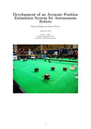
1 Overview of Thunderbots Setup . . . . . . . . . . . . . . . . . . . . . . . . . . . . . 5
2 Kalman Filter Performance without Camera Data . . . . . . . . . . . . . . . . . . 8
3 Kalman Filter Performance with Camera Data (Actual Latency=330 ms, Perceived
Latency=300ms) . . . . . . . . . . . . . . . . . . . . . . . . . . . . . . . . . . . . . 9
4 Communcation Architecture of Thunderbots Platform . . . . . . . . . . . . . . . . 11
5 State Estimation vs Camera Data for a 3-step Path . . . . . . . . . . . . . . . . . . 16
6 Step Response of X-position in Global Reference Frame . . . . . . . . . . . . . . . 17
7 Step Response of Y-position in Global Reference Frame . . . . . . . . . . . . . . . 18
8 Step Response of θ-orientation in Global Reference Frame . . . . . . . . . . . . . . 19
9 Zoomed-in Y-position Response . . . . . . . . . . . . . . . . . . . . . . . . . . . . . 20
10 Latency behavior of Camera Data versus Encoder-based State Estimation . . . . . 23
List of Tables
1 Size of elements required for time-rewinding aspect of Kalman Filter . . . . . . . . 14
2 Mean and Standard Deviation of Error in Desired Locations at steady-state . . . . 21
3 List of Deliverables and Ongoing Commitments . . . . . . . . . . . . . . . . . . . . 26
3
4. 1 Executive Summary
The UBC Thunderbots Club annually participates in the Small Size League (SSL) of the Robocup
competition, where autonomous robots play soccer in a 6-on-6 format. Based on previous experi-
ences, the robots were seen to exhibit high positional and angular errors on high speed plays due
to an inadequate position estimation system. Hence, the aim of this ENPH 479 project was to
improve the robot’s position estimation system in order to execute plays with accuracy.
Prior to this project, the robots relied on relative position commands and on-board sensor mea-
surements to determine their state during a play. This open-loop architecture led to accumulating
errors in position and angular orientation of the robots. This was changed to a closed-loop ar-
chitecture by employing a global positioning system by broadcasting camera packets containing
positions of all robots, ball, camera data latency and various status information to all robots on the
field. Simulations of a Kalman filter, a real-time & recursive algorithm to integrate camera data
and on-board sensors measurements, were conducted in MATLAB to determine its effectiveness
as a state estimation system. Delay variables (perceived and actual) were employed to account
for latency of camera data delivery to the robots, showing minor errors for latencies on the order
of 330ms and a difference in perceived versus actual latency of 30ms. The implementation of the
Kalman Filter on the robots’ firmware was found to be infeasible, and instead a latency-adjusted,
kinematics-based solution using camera and wheel-encoder measurements was implemented. The
resulting errors in positions were found to be within 1.4 millimetres of the desired positions with
corresponding variances of 2 millimetres.
The infeasibility of the Kalman Filter was largely attributed to drifting measurements on the ac-
celerometer and gyroscope sensors, introducing noise with non-zero means and therefore violating
a fundamental requirement of the Kalman algorithm. The latency of camera data was determined
through results-based tuning - measuring and reducing the jitter in angular orientation at fixed
cartesian coordinates by iterating over a range of latencies used with the state estimation algo-
rithm. Based on the magnitude of the resulting latency of ∼75ms, the main sources of latency
were found to be due to queuing of camera packets and the processing time of the computer vision
algorithms. The packet queuing latency was then accurately determined to have a mean of 25ms
with a standard deviation of 4.5ms through the use of timing functions while the computer vision
software exhibited a latency of mean 50ms with negligible variation. Accounting for this latency in
the state estimation algorithm was found to reduce the standard deviation of error in the angular
orientation of the robots, from 1.4◦
to 0.6◦
.
Elimination of sensor drift on the robots would allow for revisiting the Kalman Filter, leading
to potentially better state estimation. Moreover, other forms of the Kalman Filter such as the
Extended Kalman Filter could be used to account for nonlinearities in the robot’s dynamics.
Implementation of time synchronization protocols over the entire Thunderbots ecosystem would
provide more accurate measures of end-to-end latency and in turn, result in a better state estima-
tion system. Lastly, improvements in the dynamics of the robot impacted by design defects and
wheel slippage would lead to better response.
4
5. 2 Introduction
The UBC Thunderbots team develops soccer-playing robots to compete in the Small Size League
of the Robocup competition every year. Matches take place in a 6-on-6 format with overhead
cameras on the field, and a central computer relaying positions for all robots and the ball to each
of the team’s computers. This information is then used by each team to initiate the required plays.
Figure 1: Overview of Thunderbots Setup
The current platform at Thunderbots uses the position data to assign relative position commands
and primitives to each of the robots in order to execute these plays, as the robots are unaware
of their global positions on the field. On-board sensors are used to determine the state of the
robots (position, velocity and acceleration) during a play, using simple kinematic relations. Based
on reviews of last year’s performance, it was observed that robots were highly inaccurate on high-
speed plays (∼ 2m/s), due to accumulation of error during a play and the absence of a mechanism
to correct for mid-play errors i.e. open-loop system. This is the basis for the development of an
accurate global position estimation system for the robots.
In order to solve this problem, we proposed to deliver the global position data obtained from
the central computer, completely downstream to the firmware on the robots. Broadcasting this
data continuously (∼ 30 packets per second) would allow for correction of accumulated errors given
that the errors in camera data were established to be a few orders of magnitude lower than the
on-board sensors on the robots. Moreover, since Kalman filters are used widely in navigation ap-
plications to combine various sensor inputs with different variances to determine the best estimate
of state and the corresponding uncertainties, we chose to apply it to the camera data and the
outputs of the on-board sensors.
Hence, the project objectives could be summarized as follows.
• Simulation of Kalman Filter (with delay variables to account for latency) to determine effec-
tiveness of solution
• Implementation of Camera Packet handling threads and functions (to segregate it from the
rest of the software stack on each of the team’s computer)
• Implementation of Radio Communication to broadcast Camera Data to the robots
5
6. • Implementation of the State Estimation Algorithm on the robot firmware
• Testing and Tuning of time delay variables to account for data communication latencies
An aspect of the project that was eliminated after the proposal stage was the time synchronization
of the clocks between the team’s computer and the microcontroller on the robots. This was done
due to a number of reasons:
1. Unsynchronized clocks also exist between the central and team’s computers, and the NTP
protocol could not be used due to lack of internet connectivity. This same applies to the
team’s computer and the microcontroller on the robot
2. Inability to eliminate or account for transmission-side delays associated with interrupts and
event handling due to unsupported MAC Layer timestamping on radio transceiver modules
3. Other time synchronization protocols would require additional hardware (e.g. IR beacons to
signal an event) and too extensive for the duration of this project.
While time synchronization implementations would have allowed for accurately determining the
delays (most protocols allow for accuracies on the order of a millisecond) in the capture of an im-
age and its transmission to the microcontroller to use in the Kalman filter, simulations performed
for variations up to 10% in the perceived delay versus the actual delay (330 ms or less) for data
delivery did not affect the results to any significant extent. A 330 ms value for the time delay
was quoted by former members of Thunderbots, however, this claim was falsified through tuning
procedures which revealed a latency on the order of 35ms, which could be mostly accounted for by
the camera packet queuing on the AI layer.
In the following sections, we will describe and explain the methods, results and recommenda-
tions for each of the listed project objectives in the stated order. Methods of debugging and/or
verification of the results are also detailed. In the final sections, we will conclude with the state of
the project and the extent to which the primary objective was achieved - to provide an accurate
position estimation for the robots - with suitable metrics, as well as recommendations and ongoing
commitments to build upon our work.
6
7. 3 Kalman Filter Simulation
This section describes the simulation of a Kalman Filter to estimate the state of a single robot
subject to specified accelerations. We present a time-delayed Kalman Filter to account for latencies
in camera data.
The results and analysis are conducted for representative maximums in data latency, in order
to determine the worst-case scenarios for the performance of the system.
3.1 Theory
Kalman filtering, also known as linear quadratic estimation (LQE), is an algorithm that uses a
series of measurements observed over time, containing statistical noise and other inaccuracies, and
produces estimates of unknown variables that tend to be more precise than those based on a single
measurement alone, by using Bayesian inference and estimating a joint probability distribution
over the variables for each timeframe1
.
Without delving into the details of the derivation2
, we present the estimation and update equa-
tions that are used each time the sensor outputs are read (refer to Appendix A for the state-space
representation matrices and vectors):
Kalman Gain: Kk = Pk|k−1HT
(HPk|k−1HT
+ R)−1
Update Estimate: ˆxk = ˆxk|k−1 + Kk(zk − Hˆxk|k−1)
Update Covariance: Pk = (I − KkH)Pk|k−1
Project into k+1: ˆxk+1|k = F ˆxk + Buk, Pk+1|k = FPkFT
+ Q
In the equations above, ˆxk|k−1 and Pk|k−1 refer to the initial estimates of state and errors at
time k, based on the previous timestep.
The fundamental assumptions in the use of the standard Kalman Filter are:
• Application to a linear-time invariant system
• Measurement noise have Gaussian distributions with means of zero
3.2 Matlab Implementation
The Kalman Filter Simulation Code is provided in Appendix B.
The filter was simulated in Matlab for a single robot with two sets of state-space representa-
tion matrices - one set for the wheel encoders, accelerometers and gyroscope, and another set for
the camera data. This was required as the camera data is not read in as quickly (∼30 Hz) as
the data from the other sensors (200 Hz). This is reflected in the Kalman Update Function in
Appendix B.
The measurement covariances of the sensors defined in the simulation reflect the real values,
based on sensor datasheets provided by the manufacturers. From the comparison of the R_cam
and R_local variables, it can be seen that the measurement variance (noise) of the camera is a few
order of magnitudes lower than that of the other sensors, hence, justifying its use in the Kalman
filter to correct for accumulated errors in position.
In order to incorporate the delayed camera data, past measurements and state data are stored
(since the previous camera packet) in order to re-apply the Kalman filter update equations to
produce the present estimate of state.
1"Kalman filter - Wikipedia." https://en.wikipedia.org/wiki/Kalman_filter. Accessed 30 Dec. 2016.
2"Tutorial: The Kalman Filter." http://www.zabaras.com/Courses/UQ/kf1.pdf. Accessed 30 Dec. 2016.
7
8. 3.3 Results and Analysis
Based on the experiences of former members of the Thunderbots team, we were told that the
latency of the camera packets was on the order of 330 ms (a claim that was later debunked during
the course of this project and is described in Section 7).
Using the worst-case scenario value of 330 ms for the latency of the camera packets with a ‘per-
ceived’ camera delay of 300ms, we obtained the following results (compare against case with no
camera data in Figure 2):
Figure 2: Kalman Filter Performance without Camera Data
8
9. Figure 3: Kalman Filter Performance with Camera Data (Actual Latency=330 ms, Perceived
Latency=300ms)
A timescale of 4 seconds was chosen for the simulation as it is representative of a typical play/prim-
itive instruction, and hence would exhibit expected deviations in end positions. Moreover, accel-
erations were varied over the full range of 3 m/s2
(maximum acceleration the robots can achieve)
to characterize the ‘high-speed’ plays where errors are most significant.
The Kalman Position curves exhibit a 1-dimensional path that the robot ‘believes’ it is follow-
ing, while the Actual Position curves reveal the true trajectory of the robot. The additional
Corrected Kalman curve with the camera data shows the estimate of position that is corrected by
the incoming camera packets. This, in turn affects the behaviour of the Kalman Position curve.
While the above represents a 1-dimensional analysis in position, similar results are seen for angular
orientation as well. Incorrect angular orientations highly impact the shooting/dribbling of the ball
on the field due to the angle of contact of the ‘chipper’ mechanism with respect to the ball.
As can be seen from Figure 2, error accumulates over the trajectory of the robot and the po-
sition estimate deviates greatly from the actual position as compared to the results of Figure 3.
Therefore, the results justify the use of the Kalman filter in developing an accurate state estimation
system.
9
10. 4 Camera Packet Handling
4.1 System Overview
Prior to the completion of this project, the camera data was used by the AI (without any method to
account for delay) to calculate the relative distance from the robot to its destination. A movement
primitive command was then sent to the robot instructing it to move that far from its current
position.
The new implementation works differently- the camera data is handled by the AI computer and
then transmitted over radio to the robots. A separate AI thread was created to process camera
data. The vision thread is responsible for time stamping and storing the data, and the main thread
sends it over the radio.
When the Thunderbots AI is started up, this thread is created and a reference to it is stored
as a member variable of the VisionSocket object. This thread enters a while-true loop, and in each
pass it waits for an input from the vision computer using the Linux ’recv’ function with blocking
set to true. When a vision packet is received, a timestamp called ’time_recv’ is created. The
vision packet is then saved to a mutex-locked (for thread safety) queue along with the time_recv
timestamp. The vision thread loop then starts again.
The main AI loop checks the vision packet queue once per iteration. It requests the queue mutex
and then flushes the queue, handling each vision packet. The current time is compared against the
time the packet was received, and then all new robot position data is transferred over the radio
to the robots, as discussed in section 5. The measured time difference is also transmitted to the
robots. This information is useful because then the robots have a much more accurate time by
which to rewind and replay sensor data, as is described in section 6.
4.2 Debugging
This software was mainly debugged using print statements to ensure that the correct information
was being sent to the radio function. More rigorous debugging occurred simultaneously with the
testing of the radio protocol. The code has been used for several weeks with no unexplained
behaviour or crashes, ruling any threading bugs unlikely.
4.3 Results
The use of this separate thread has removed any uncertainty in the delay time that the AI imposes
on each packet. Without the thread, timestamps would be delayed between 30 and 60 milliseconds,
with no way to quantify this delay. This implementation has been found to delay the data by an
average of 25 milliseconds, with a maximum observed value of 31 milliseconds and a minimum
observed value of 18 milliseconds. This amount of time is likely not problematic when onboard
sensors are also used.
10
11. 5 Radio Communication of Camera Packets
This section describes the implementation of a new radio protocol for the Thunderbots platform,
delivering positions of the robots, the ball, timestamp and other states of the system e.g. e-stop,
completely downstream to the robots.
5.1 Communication Architecture
Figure 4: Communcation Architecture of Thunderbots Platform
The central computer transmits the camera data to each of the team’s computer using Google
Protobuf (or Protocol Buffers) messages. These messages are just a means of serializing structured
data, similar to XML and JSON. In our architecture, these messages are sent over a CAT-5 cable
to the AI computer.
These messages are then intercepted by the Camera Packet Handling thread detailed in the pre-
vious section, queuing up these data packets to be serially processed in order to initialize the bulk
of the Camera Packet messages (structure is defined in section 5.2).
The mostly initialized Camera Packets are then sent over to the radio dongle connected to the
computer via a USB protocol. The rest of the Camera Packet fields are initialized at this stage e.g.
estop is directly connected to the dongle and so the estop field is assigned in the camera packets
here.
The fully assigned packets are then broadcasted to the radio dongles of all the robots on the field.
Upon receipt of the camera packets, interrupts are generated by the dongle to the microprocessor,
triggering the decoding sequence and subsequent use of the packets.
5.2 The Camera Packet
The Camera Packet is a variable-size data structure depending on the availability of valid posi-
tion/angular data for the robots and the ball, and depending upon the status of the emergency
stop switch. This was a requirement in order to minimize the bandwidth consumption on the radio
channel. There are a maximum of 8 robots that can be on the field at any time (to justify the use
of bit masking for certain bytes in the camera packet).
The structure of the Camera Packet can be summarized as follows:
11
12. 1. Flag Vector (Byte 1) - A bit-masked byte with the first 3 bit positions corresponding to the
state or validity of the emergency stop, timestamp and ball positions
Bit Flag
3-7 Reserved
2 Does packet contain a ball position?
1 Does packet contain a camera timestamp?
0 Emergency Stop flag
2. Mask Vector (Byte 2) - A bit-masked byte with bits set in positions corresponding to Robot
IDs if valid position data exists for those robots
3. Ball X Position (Bytes 3-4) - A 2-byte representation of the ball’s x cartesian coordinates on
the field (in mm)
4. Ball Y Position (Bytes 5-6) - A 2-byte representation of the ball’s y cartesian coordinates on
the field (in mm)
Word Value
0 Ball’s global x-position, in mm
1 Ball’s global y-position, in mm
5. 8 x Robot Position (Bytes 7-54) - Each robot position is given by a 6-byte structure, with 2
bytes each for the Robot’s x, y (both in mm) and θ (in milliradians) coordinates
Word Value
0 Robot’s global x-position, in mm
1 Robot’s global y-position, in mm
2 Robot’s signed global angle position, in milliradians
6. Timestamp (Bytes 55-62) - An 8-byte timestamp that currently relays the time delay/latency
(in ms) associated with the queuing and sending of the camera packets
7. Status Byte (Byte 63) - First 3 bits are used to denote the Robot ID that is required to
return a status message
12
13. Bits Value
3-7 Reserved
2-0 Robot number
5.3 Debugging
In the debugging phase, we wished to ensure that packets were being received on the robot firmware
and packets were complete and followed the rules dictated by their variable sizing.
The firmware on the robot provides SD Card logging facilities, through the passing of logger
objects between different tasks in the firmware. The logger object was passed into the receiving
side of the radio code (which is invoked upon registering an interrupt from the radio transceiver
module) to log all the bytes of the incoming camera packets.
Once written on, the SD card does not retain its default filesystem e.g. NTFS, FAT32. It registers
data in the form of epochs, where data is merely written into sectors of memory on the SD card.
After logging the data and transferring the card to a computer, the sdutil binary (available on-
line) was used to generate a spreadsheet (.tsv) file to view the data in any commercial spreadsheet
software.
The bytes logged by the radio receiving code onto the SD card were inspected based on differ-
ent conditions i.e. with and without ball data, different estop states, different numbers of robots
on the field etc. Once all cases were verified, we proceeded to test the implementation with robots
on the field.
5.4 Testing and Results
In order to verify the working behaviour of the radio code and its integration with the rest of
the firmware, plays were executed for the robot to move to specific end locations on the field.
As expected, the robots moved to the specified positions, thus verifying the correctness of the
implementation of the radio protocol. At this stage, the errors in positions and orientations were
not important and so, no quantitative data is presented here.
13
14. 6 Implementation of State Estimation Algorithms
This section describes the framework and implementation of the Kalman filter and its failings
in delivering an effective state estimation system. A second approach based on kinematics and
the integration of camera data with wheel encoder measurements that was ultimately used in the
project is detailed.
6.1 The Kalman Filter
As mentioned throughout this report, the Kalman Filter was to be the algorithm of choice in inte-
grating the camera data and measurements from the accelerometer, gyrosocope and wheel encoders
in delivering a state estimation system for the Thunderbots platform.
However, certain problems were encountered (detailed below) that led to the infeasibility in using
the Kalman filter as an effective solution.
6.1.1 Framework
The framework for the Kalman filter was developed by the current electrical lead of the Thunder-
bots team, Ryan de Laco. This was still in its experimental stages and a work in progress prior to
the merging of his work in our project.
The framework for the Kalman Filter uses the sensors and camera data to update state variables
on the robot, before calling on a Kalman step to run the state estimation and update equations
as described in the simulation section and Appendix A. The results of the Kalman filter are then
stored and used by the controller code and the like.
6.1.2 Firmware Implementation
The firmware code for the Kalman filter can be seen in Appendix C.
Required matrix operations were implemented without the use of third-party libraries in order
to conserve memory space. Also, the measurement covariance matrices (Q_x, Q_y and Q_t) are
multiplied by the length of the timestep in order to adjust for the process noise error. A linear
scaling with the length of the timestep is justified by the following statistical rationale:
Linear Scaling of Error with Timestep
Let Xt = Xt/2 + Xt/2 , where Xt represents the process noise over a period t which is in
turn given by the process noise over 2 periods of half the length. It is reasonable to assume
both Xt/2 to be i.i.d (independent and identically distributed) random variables.
So V ar(Xt) = V ar(Xt/2) + V ar(Xt/2) = 2V ar(Xt/2). This can be more generally
stated as, V ar(Xt) = n ∗ V ar(Xt/n). Hence, we can deduce that the process noise
covariance matrices will scale with the length of the timesteps.
The time-rewinding aspect of the Kalman filter in the simulation required storage of various ele-
ments (detailed in the table below) at every timestep since the last obtained camera packet.
Parameters Declaration Size of Type (bytes) Total Size (bytes)
States float x_x[3], x_y[3], x_t[3] 4 36
Estimate Variance Matrices float P_x[3][3], P_y[3][3], P_t[3][3] 4 108
Measurements float z[3] 4 12
Inputs float x_accel, y_accel, t_accel 4 12
Table 1: Size of elements required for time-rewinding aspect of Kalman Filter
Based on the latency of ∼75 ms determined later in the project (see section 7), this would require
a storage of storage of 36+108+12+12 = 168 bytes at every run of the control loop (which runs
at 200 Hz). Hence, a memory space of at least 168 * 200 * 0.075 = 2.46 kB would be required for
14
15. this aspect, which is well within the available SRAM size of 24 kB for the ARM Cortex M4 MCU
used on the robots.
6.1.3 Testing and Results
The C Kalman code was debugged using multiple print statements in the Kalman step function. A
MATLAB function was written with identical matrix operations as the C function for every line.
These two functions were compared to validate each step of the process. Several errors were found
in the C matrix multiplication and inversion functions being used. The overall update of the state
and covariance matrix was made to match the MATLAB function when the same input matrices
were used.
The Kalman firmware was tested on the robot with actual camera and sensor data. The move-
ments of the robot were not as expected- it would move rapidly to some point relatively close to
the destination (approx. 30cm), hover there for a few seconds, then move rapidly to another point
also close to the destination. The location of the destination was constant, and to all appearances
there was nothing to predict when the robot would rapidly move to the next position. Due to time
constraints and the success of a simpler algorithm (discussed in section 6.2) the Kalman filter was
not developed further.
6.1.4 Issues
From the logging of accelerometer and gyroscope data on the robot (only one was available for
testing), it was seen that they were highly inaccurate and exhibited significant drift in their out-
puts. This in-turn meant that the “noise” or error on the sensor was distributed normally with a
non-zero mean. However, this violates the fundamental assumption of the Kalman Filter requiring
that the errors from sensors be distributed around a mean of 0, and so ruling out the use of the
Kalman Filter as a feasible solution.
While it was possible to use just the wheel encoder and camera data in the Kalman Filter, it
would result in unnecessary complexity for only one sensor measurement. Another failing of the
Kalman Filter in the current circumstance was that on-board sensor measurements provided mea-
surements relative to the reference frame of the robot while camera measurements were in the
global reference frame. This meant that a conversion was required from one reference frame to
another based on the current angle of the robot. This violates the other fundamental requirement
of the Kalman Filter which requires that measurements be independent of the current state of the
robot.
6.2 Latency-Adjusted Kinematics Solution
Based on the issues with the sensor described above, we decided to proceed with the use of only
the camera packets and the wheel encoders in developing the position estimation system.
The alternative solution that was eventually implemented is described in the sections below.
6.2.1 Algorithm
The algorithm assumes a non-zero latency in the camera packets, which is later determined and
set based on the results of the tuning procedure detailed in section 7.
The algorithm maintains a list of the latest robot speeds as measured by the wheel encoders.
When a camera packet is obtained, wheel encoder speeds from some time in the past that is de-
termined by the latency variable, are integrated and added to the position data obtained from the
camera.
Since, the wheel encoders report speeds in the reference frame of the robot, they are converted to
global coordinates by the application of rotation matrices based on the current angle estimate of
the robot. This is done during each step of the integration based on the best estimate of robot
direction at the time the wheel encoder measurement was made.
15
16. 6.2.2 Implementation
The list/buffer for the speeds reported by the wheel encoders was implemented through the use of
a circular buffer - a fixed size array with pointer variables that are incremented circularly as data
is added to the array. This buffer is accessed using a method that reads the data from a specified
time in the past.
The sensors are sampled and used at fixed intervals of 5ms that are generated from timer inter-
rupts on the microcontroller. This provides the integration time between successive wheel encoder
speeds in order to estimate current position and angular orientation of the robots.
As with the rotation of the encoder speeds by the current angle estimate of the algorithm, the
control algorithms used by the robot also require defining the displacement of the robot with
respect to the desired location in the robot’s reference frame. In order to achieve this, the differ-
ence in the desired location and the current position estimate of the robot, both defined in global
coordinates, is rotated by the current estimate of angle for the control calculations.
6.2.3 Testing and Results
With the appropriate values of latency in place, the robot was tested by requiring it to perform
a 3-step maneuver ending at the initial location. In order to quantify the performance of the
implemented algorithm, differences between the desired locations and the means of the achieved
steady state positions at each step, as well as the jitter/variance in the position and angular
orientation of the robot at each location were determined. This was achieved by logging the camera
data and the robot’s state estimates using an SD card and performing the required analysis using
the R data analysis software.
Figure 5: State Estimation vs Camera Data for a 3-step Path
Figure 5 shows the position of the robot as it follows the 3-step path. Blue lines denote estimated
position and black dots are camera measurements. It can be seen that the robot follows a very
consistent path, with small recurring errors in the trajectory followed and position estimation. The
reason for both of these problems is believed to be wheel slippage. Independent tests by mechanical
16
17. and electrical team members have revealed that the base plate of the robot is misaligned and that
the front left wheel of the robot often is not in contact with the ground, especially during periods
of high acceleration. This component of the problem has been deemed outside the scope of the
project. In the future, mechanical improvements will be made. Despite this deficiency, it has been
observed that robot control performance has improved significantly.
The following three graphs show how x position, y position, and angle change over time during the
maneuver.
Figure 6: Step Response of X-position in Global Reference Frame
17
18. Figure 7: Step Response of Y-position in Global Reference Frame
18
19. Figure 8: Step Response of θ-orientation in Global Reference Frame
19
20. These graphs demonstrate the stability of the resultant system. There is very little overshoot or
oscillation, and the response time of the system is quite fast given that the robots have a maxi-
mum velocity of 2m/s. The estimate matches the camera data quite well for most stages of the
maneuver. Exceptions are believed to be due to wheel slippage.
Figure 9 shows the y position over a two second interval to give a more detailed view of how
the estimate tracks camera measurements.
Figure 9: Zoomed-in Y-position Response
It can be seen that the camera data lags the position estimate, as it was designed to do. The
camera function exhibits steps because new data only arrives every 30ms (opposed to a robot tick
time length of 5ms). The estimated position is fairly smooth, with only a few vertical adjustments
due to an unexpected camera data point (which is believed to be due to the wheel slippage prob-
lem discussed before). The position doesn’t overshoot the destination at all for this stage, and it
stabilizes to the correct position quite quickly.
The steady state behaviour of the system is a very important property of the overall design. The
robot must be able to reach an accurate position and angle in order to perform precise movements
with the ball, like shooting it at a small target across the field. The steady state position errors
from the three stages of the maneuver are shown in Table 2 below.
20
21. Step 1 (0 m, 0 m, 0 rad) Step 2 (0.7 m, -0.7 m, 0 rad) Step 3 (2 m, 1 m, 0.3 rad)
Mean Error, x -1.47 mm 1.22 mm -0.22 mm
Mean Error, y -0.42 mm -0.87 mm -0.36 mm
Mean Error, θ 0.82 degrees 0.035 degrees -0.10 degrees
Error Std, x 1.75 mm 2.54 mm 0.88 mm
Error Std, y 2.0 mm 1.86 mm 2.24 mm
Error Std, θ 1.06 degrees 0.93 degrees 0.87 degrees
Table 2: Mean and Standard Deviation of Error in Desired Locations at steady-state
It has been demonstrated that the steady state positional error has been reduced to the order of
2mm and the steady state angular error has been reduced to the order of 1 degree. These values are
quite close (within 50%) of the tolerances given by the vision system, suggesting that the steady
state error is almost as low as it can feasibly be made while using the current sensors. These
tolerances are more than sufficient for precise movements with the ball.
21
22. 7 Tuning for End-to-End Camera Packet Latency
This section describes the determination of the total end-to-end latency of the camera packets as
well as the sources of latency inferred from the results. The results of this section were employed
for the latency adjustment of the state estimation algorithm detailed in section 6.2.
7.1 Tuning Methodology
Since it was not possible to implement time synchronization protocols across the entire Thunder-
bots ecosystem i.e across the central computer, team computers and the robots, due to infeasibility
in implementing NTP protocols (no internet access) and lack of an advanced radio transceiver mod-
ule that is capable of timestamping messages at the MAC layer, we approached tuning for latency
using a results-based method.
Initial tests were conducted with the robot being required to move to desired end positions using
wheel encoder data alone. It was seen that while errors were present in each of the desired states
(position and angular orientation) there was hardly any jitter in the orientation of the robot as
it achieved it’s believed desired position. However, testing the state estimation algorithm with an
out-of-tune latency estimate produced considerable jitter which evolved into instability for certain
guesses of latency. Based on the documentation of the computer vision software at Thunderbots,
the standard deviation of the angular positions reported by the camera are on the order of 1 de-
gree. Hence, it was fair to assume that the jitter produced was due to unaccounted latency in the
camera data. Moreover, the jitter appeared to lead to a condition of angular instability due to the
mismatch in timing of the camera data and the control algorithms.
This results based approach for the tuning can be summarized as follows:
1. Robot given a desired end location and orientation different from initial state
2. At end position, robot iterates through a range of latency guesses, staying at each guess for
a period of time (∼ 5 seconds) to observe the results
3. Robot is timed using stopwatch to determine the iteration at which the most stable behaviour
was seen
4. Successively reduce the iteration interval, similar to root-finding using the bisection method
5. Based on the required tolerance for the latency, stop iterating when the iteration interval is
reduced to the size of the tolerance
7.2 Results and Analysis
As the robot iterated through the latency ranges, the transition from unstable to stable and back
was quite evident, with the angular jitter being very small and the angular orientation being highly
accurate (within 1 degree) of the required orientation.
After successive iterations of the ranges of the latency guesses, we found the latency to be on
the order of 60 ms (much smaller than the so claimed 330 ms!). Based on the handling of the cam-
era packet detailed in section 4, the packets are queued and processed at a rate of 30 packets/sec,
which corresponds to 33.3 ms/packet. Hence, it was fair to believe this to be a significant source
of the latency. In order to verify our suspicions, timing functions were used in the camera packet
handling code to determine the time between the queuing of the packets and the time they were
processed. The resulting statistical averages and standard deviations of this process were found to
be:
¯t = 25ms, σt = 4.5ms
Any additional sources of latency were assumed to be a result of the computer vision processing
on the central computer. This was assumed to be constant, due to it being a more deterministic
process with a multi-threaded implementation for handling multiple incoming raw images (refer to
SSL-Vision documentation3
for details on the computer vision software).
3"SSL-Vision: The Shared Vision System for the RoboCup Small ... - DFKI."
https://www.dfki.de/web/forschung/publikationen?pubid=5268. Accessed 6 Jan. 2017.
22
23. The tuned latency of 60 milliseconds is validated by the following analysis comparing encoder
and camera data stored simultaneously on the robot. The robot is given commands to change its
angle rapidly. After several of these movements have been performed the logged data is graphed.
Figure 10 shows the angular position over time as measured by the camera and the wheel encoders
(initially set to match values). The wheel encoder time series was manually shifted in time until
it best matched the camera time series. This occurs when the delay time is set to 75 ms, as shown
by the blue line in the graph.
The combination of tuned value and compared data provide strong evidence for a delay time
between 60 and 75 ms. On average 25 of the milliseconds are believed to be caused by the delay in
AI. The remaining latency is likely due to the computer vision algorithm. Based on these findings,
the robots apply a delay time with a base value of 35 milliseconds and a variable value equal to
the delay AI reports.
Figure 10: Latency behavior of Camera Data versus Encoder-based State Estimation
Based on the logging of test data on the SD card for robots required to move to desired positions
and orientations, the jitter in the angular orientations of the robots was found to exhibit an angular
standard deviation of 0.6°. Based on the analysis of robots from game logs (positions and angular
orientations of robots during play are logged by the camera data on the AI computers for games
played during all competitions), the robots previously displayed multiple modes of instability such
as not settling in a position (positional) or continuously turning in place (angular instability).
For trajectories where robots did exhibit stable behaviour, the standard deviation of the angular
23
24. jitter was calculated to be 1.4°. Hence, we can see that considerable improvement in the state
estimation system has been achieved through reduction of the angular variation of the robot from
1.4° to 0.6°. Moreover, the step responses shown in section 6.2.3 which were obtained after the
implementation of the tuning, display steady state behaviour unlike the older step responses which
typically exhibited indefinite steady state times.
24
25. 8 Conclusion
Simulations of a Kalman Filter in MATLAB, using sensor measurements and camera data, with
variable latency and variable ‘perceived’ latency revealed that differences between the two (meant
to represent errors in determining latency) on the order of 30 ms resulted in end position and
orientation deviations on the order of as opposed to the errors of for an open-loop control system
(without camera data).
A new radio protocol was developed to broadcast camera packets containing positions and an-
gular orientation of all robots, the ball, processing latencies and other system state variables to
robots on the field. Initialization of the variable-sized camera packets is done through means of a
camera data handling thread to queue incoming position and orientation data received from the
computer vision software, and define the required fields of the packets. Debugging and testing
was performed through logging of packets received on an SD card and through field-testing of the
robots to move to desired end locations and orientations.
Implementation of the Kalman Filter proved impractical and unfeasible due to violation of the
assumption of the algorithm - measurements are independent of state and that the noise is dis-
tributed with zero mean. A kinematics based solution was implemented through treating camera
and wheel encoder data to be ideal, and adjusting for latency of the camera data. The results
showed that the end location deviations were down to from and angular orientation deviations/jit-
ter at steady state was down to from .
The latency of the camera packets was determined through results-based testing, with the robot
iterating through guesses of latency and quantifying the jitter of the angular orientation of the
robot at a fixed location. The quantification of latency was performed in a manner similar to the
root-finding procedures of a bisection method and found to be in the neighbourhood of 60 ms.
The primary source of the error was found to be due to the queuing of camera packets on the AI
layer, with a mean time delay of 25 ms and standard deviation of 4.5 ms. These varying latency
values are forwarded via the camera packets to the robots and added to a constant value of 50 ms
representing the latency of the computer vision algorithms, justified by their deterministic nature
and multi-threaded implementation.
25
26. 9 Project Deliverables
This section details the deliverables at the conclusion of ENPH 479 and commitments to the
Thunderbots Club that will extend beyond the end of the course. A financial summary is not
presented as no costs were incurred in the development of this project.
9.1 List of Deliverables and Ongoing Commitments
The following table summarizes the list of deliverables to the Thunderbots club available at the
end of the project and the state of these deliverables. Any necessary changes and/or additions
that are detailed in the ‘State’ of these deliverables represent the ongoing commitments to the
Thunderbots club to ensure that our work integrates seamlessly with their platform and is usable
in competition play.
Deliverable State
Matlab Simulation of Kalman Filter Complete
C++ Code for Camera Data Handling Mostly complete; Needs integration with AI stack
C++ Code for Camera Packet Initialization and
USB transfer
Complete
C Code for transmission side of Radio Protocol Complete
C Code for receiving side of Radio Protocol Complete
C Code for Kalman Filter Partially Complete; Needs further investigation with
reliable sensor measurements and/or other Kalman
Filter forms
C Code for Latency-Adjusted Kinematics-based
State Estimation
Mostly Complete; Needs some code cleanup
Documentation of Tuning and Tuning code Partially Complete
Documentation of Radio Protocol Complete
Table 3: List of Deliverables and Ongoing Commitments
26
27. 10 Recommendations
A couple of potential improvements that could be made to the position estimation platform based
on the results of the project are:
10.1 Wheel Slip Detection
Wheel slippage is a problem that is well-known at Thunderbots, however no counter-measures
against it have been implemented as of yet. We can determine when wheels are slipping by
comparing four encoder speeds against the three degrees of freedom, and gyroscope data. If they
are slipping, another method to update state and temporarily reduce the acceleration of the motors
should be used. By implementing wheel slip detection, the maximum acceleration can be increased,
which in turn would lead to improvements in the responsiveness of the robots.
10.2 Controller Improvements
Given the relatively poor state estimation system on the robots prior to the project, it is likely
the controller was not optimally tuned. Re-tuning the controller and/or implementation of better
controllers would greatly improve the performance of the robot on the field. With our state
estimation in place, significant overshoots on the order of 10 cm were observed in the approach to
desired locations on the field.
10.3 Symmetric Robot Geometry
The robot weight distribution is not symmetric because of an odd number of capacitors and an
improperly machined motor mount. It is believed that this asymmetry causes the robots to drive
in a skewed direction when reliant on the front left wheel. Either fixing this mechanically or
accounting for the asymmetry in the control logic will likely solve this problem.
10.4 Time Synchronization Protocols
Implementation of time synchronization protocols between all the devices on the Thunderbots
platform i.e. the central computer, team’s computer and the microcontroller, would allow for
determining the latencies in the delivery of camera packets to a higher degree of accuracy. It
was due to hardware and network restrictions (no internet access on devices) that such measures
could not be implemented. However, there do exist other protocols that could be implemented
with the introduction of additional hardware and communication between all the devices on the
platform e.g. having a beacon transmit to all devices and subsequent sharing of the time the
beacon event was registered on each device. Given the time restrictions on this project, such time
synchronization protocols could not be explored.
10.5 Kalman Filter Improvements
As it stands, some robots were unbalanced due to the reasons detailed in section 10.3. It would
be worthwhile to determine any other characteristics of the electrical/mechanical systems on the
robots that would result in significant non-linear dynamic behaviour. If such behaviour exists,
looking into other forms of the Kalman Filter that account for nonlinearities such as the Extended
Kalman Filter (EKF) would be valuable.
A State-Space Representation of Kalman Filter
The application of the Kalman filter requires that a system be linear-time invariant (or approxi-
mately linear-time invariant in the region of operation), with respect to its inputs and state vector.
Systems meeting this criterion can be expressed mathematically as:
xk = Fxk−1 + Buk + wk
where,
27
28. xk = state vector at time k
xk−1 = state vector at time k-1
uk = input vector
wk = process noise vector (assumed constant over time)
F = state transition matrix between time steps
B = input to state conversion matrix
The observations of state must also be linear-time invariant.
zk = Hxk + vk
where,
zk = observation vector (measurement from sensors)
vk = measurement noise vector (assumed constant over time)
H = noiseless state to measurement conversion matrix
The linear-time invariant properties require that the matrices F, B and H are constant over time.
An additional three matrices are defined for the Kalman filter:
Q = E[wkwk
T
]
R = E[vkvk
T
]
Pk = E[(xk − ˆxk)(xk − ˆxk)T
]
where ˆxk = output state estimate of Kalman filter at time k
Q and R represent the covariance matrices for the process and measurement noise respectively
and are assumed to be stationary over time. Pk is the covariance matrix for the error in state that
is updated at each timestep. It is the trace (the sum of diagonal elements) of Pk that is to be
minimized at each step to produce the optimal estimate of state.
B Kalman Filter Simulation Code
B.1 Simulation Loop
1 TIMESTEP = 1/100;
2 MAX_TIME = 4; % end of simulation
3 STEPS = round (MAX_TIME/TIMESTEP) ;
4 CAMERA_DELAY = 0 . 3 3 ; % Time in past that camera measures p o s i t i o n
5 PERCEIVED_CAMERA_DELAY = 0 . 3 ; % Camera delay used in kalman f i l t e r
6 CAMERA_FREQUENCY = 30; % measurements per second
7
8 %the s t a t e update matrix ( get next s t a t e given current one
9 F=[1 TIMESTEP 0.5∗TIMESTEP^2; 0 1 TIMESTEP; 0 0 0 ] ;
10
11 %input to s t a t e update matrix
12 B = [ 0 ; 0; 1 ] ;
13
14
15
16 % Process noise f o r process of length one second ( covariance approximated
17 % as zero )
28
29. 18 X_VAR = [ 0 . 0 5 ^ 2 ; 0.2^2; 0 . 2 ^ 2 ] ;
19
20 %the s t a t e measurement operator
21 H_cam= [1 0 0 ] ;
22 H_local= [0 , 1 , 0; 0 , 0 , 1 ] ;
23
24 %Measurement covariance − to be measured l a t e r
25 R_cam = [ 0 . 0 0 4 ^ 2 ] ;
26 R_local = [0.05^2 , 0 ; 0 , 0 . 0 1 7 ^ 2 ] ;
27
28 %the s t a t e vector over time , both the kalman estimation and the r e a l value
29 %x ( 1 , : ) − p o s i t i o n s
30 %x ( 2 , : ) − v e l o c i t i e s
31 %x ( 3 , : ) − a c c e l e r a t i o n s
32 x r e a l=zeros (3 ,STEPS) ;
33 xguess=zeros (3 ,STEPS) ;
34
35 %the s t a t e vector over time , both the kalman estimation and the r e a l value
36 %x ( 1 , : ) − p o s i t i o n s
37 %x ( 2 , : ) − v e l o c i t i e s
38 %x ( 3 , : ) − a c c e l e r a t i o n s
39 x r e a l=zeros (3 ,STEPS) ;
40 x=zeros (3 ,STEPS) ;
41 xused=zeros (3 ,STEPS) ;
42 z=zeros (2 ,STEPS) ;
43
44 %s t a r t estimate covariance (’shouldnt r e a l l y matter in steady s t a t e )
45 P = zeros (3 ,3 ,STEPS) ;
46 P( : , : , 1 )= eye (3) ;
47
48
49 %something to keep track of time
50 t=zeros (1 ,STEPS) ;
51
52 a = 3∗ s i n ( ( 1 :STEPS) ∗TIMESTEP∗5) ;
53
54
55
56
57 f o r i =2:STEPS
58
59 t ( i ) = t ( i −1)+TIMESTEP;
60
61 i f ( mod( t ( i ) ,1/CAMERA_FREQUENCY) < TIMESTEP && t ( i ) > CAMERA_DELAY && t ( i ) >←
PERCEIVED_CAMERA_DELAY)
62
63 % Get data at the actual camera delay time
64 steps_back = c e i l (CAMERA_DELAY/TIMESTEP) ;
65 picture_time = t ( i ) − CAMERA_DELAY;
66 T1 = t ( i − steps_back ) ;
67 T2 =t ( i − steps_back +1) ;
68 Weight1 =(picture_time − T1) /TIMESTEP;
69 Weight2 =(T2 − picture_time ) /TIMESTEP;
70
71 cam_pos = Weight1∗ x r e a l (1 , i−steps_back ) + Weight2∗ x r e a l (1 , i − steps_back←
+1) ;
72 cam_pos = cam_pos + randn (1) ∗R_cam. ^ ( 0 . 5 ) ;
73
74 % Steps to go back in time to apply data ( based on perceived delay )
75 steps_back = c e i l (PERCEIVED_CAMERA_DELAY/TIMESTEP) ;
76 perceived_picture_time = t ( i ) − PERCEIVED_CAMERA_DELAY;
77 j = i − steps_back + 1;
78
79 [ xtemp , Ptemp ] = kalmanUpdate ( x ( : , j − 1) , P ( : , : , j − 1) , a ( j − 1) , z ( : , j ←
−1) , perceived_picture_time − t ( j − 1) , f a l s e ) ;
80
81 [ x ( : , j ) , P ( : , : , j ) ] = kalmanUpdate (xtemp , Ptemp , a ( j −1) , cam_pos , t ( j ) − ←
perceived_picture_time , true ) ;
82
83 f o r j = ( i − steps_back + 2) : ( i − 1)
84 [ x ( : , j ) , P ( : , : , j ) ] = kalmanUpdate (x ( : , j − 1) , P ( : , : , j − 1) , a ( j − 1) ,←
z ( : , j −1) , TIMESTEP, f a l s e ) ;
85 end
29
30. 86 end
87
88 %actual model run to simulate t h i s time step
89 x r e a l ( : , i ) = F∗ x r e a l ( : , i −1) + B∗a ( i ) + randn (3 ,1) . ∗ (TIMESTEP∗X_VAR) . ^ ( 0 . 5 ) ;
90
91 % Measurement i s based on r e a l values , and e r r o r s due to sensors
92 z ( : , i ) = H_local∗ x r e a l ( : , i ) + randn (2 ,1) . ∗ ( R_local ∗ [ 1 ; 1 ] ) . ^ ( 0 . 5 ) ;
93
94 [ x ( : , i ) , P ( : , : , i ) ] = kalmanUpdate (x ( : , i −1) , P ( : , : , i −1) , a ( i ) , z ( : , i ) , ←
TIMESTEP, f a l s e ) ;
95 xused ( : , i ) = x ( : , i ) ;
96 end
97
98
99 f i g u r e ()
100 plot ( t , xused ( 2 , : ) , ' r ' , ' linewidth ' , 2)
101 hold on
102 plot ( t , x r e a l ( 2 , : ) , ' linewidth ' , 2)
103 legend ( 'Kalman Velocity ' , ' Actual Velocity ' )
104 x l a b e l ( 'Time ( s ) ' , ' f o n t s i z e ' , 12) ;
105 y l a b e l ( ' Velocity (m/ s ) ' , ' f o n t s i z e ' , 12) ;
106 t i t l e ( ' Velocity vs Time ' , ' f o n t s i z e ' , 14)
107 hold o f f
108
109 f i g u r e ()
110 plot ( t , xused ( 1 , : ) , ' r ' , ' linewidth ' , 2)
111 hold on
112 plot ( t , x r e a l ( 1 , : ) , ' linewidth ' , 2)
113 plot ( t , x ( 1 , : ) , ' g ' , ' linewidth ' , 2)
114 t i t l e ( ' Position vs Time ' , ' f o n t s i z e ' , 14)
115 y l a b e l ( ' Position (m) ' , ' f o n t s i z e ' , 12) ;
116 x l a b e l ( 'Time( s ) ' , ' f o n t s i z e ' , 12) ;
117 legend ( 'Kalman Position ' , ' Actual Position ' , ' Corrected Kalman ' )
118 hold o f f
B.2 Kalman Update Function
1 function [ x , P] = kalmanUpdate ( x0 , P0 , u , z , TIMESTEP, camera )
2
3 i f ( camera == true )
4 H = [1 0 0 ] ; %the s t a t e measurement operator
5 R = [ 0 . 0 0 4 ^ 2 ] ; %Measurement covariance
6 e l s e
7 H= [0 , 1 , 0; 0 , 0 , 1 ] ; %the s t a t e measurement operator
8 R = [0.05^2 , 0 ; 0 , 0 . 0 1 7 ^ 2 ] ; %Measurement covariance − to be measured l a t e r
9 end
10
11 %the s t a t e update matrix ( get next s t a t e given current one
12 F=[1 TIMESTEP 0.5∗TIMESTEP^2; 0 1 TIMESTEP; 0 0 0 ] ;
13
14 %input to s t a t e update matrix
15 B = [ 0 ; 0; 1 ] ;
16
17
18 % Process noise f o r process of length one second
19 X_VAR = [ 0 ; 0.2^2; 0 . 2 ^ 2 ] ;
20
21 %The amount of uncertainty gained per step
22 Q= TIMESTEP ∗ diag (X_VAR) ; %covariance approximated as zero
23
24 %p r e d i c t the current s t a t e and covariance given previous measurements
25 xtemp = F∗x0 + B∗u ;
26 Ptemp = F∗P0∗F' + Q;
27
28 %how much does the guess d i f f e r from the measurement
29 r e s i d u a l = z − H∗xtemp ;
30
31 %The kalman update c a l c u l a t i o n s
32 Kalman_gain = Ptemp∗H' / (H∗Ptemp∗H' + R) ;
33 x = xtemp + Kalman_gain∗ r e s i d u a l ;
30
31. 34 P = ( eye (3) − Kalman_gain∗H) ∗Ptemp ;
35
36 end
C Kalman Filter Firmware Code
1 #include "kalman . h"
2 #include <s t d i o . h>
3 void print_mat ( unsigned i n t rows , unsigned i n t cols , f l o a t X[ rows ] [ c o l s ] ) {
4 f o r ( unsigned i n t i = 0; i < rows ; i++){
5 f o r ( unsigned i n t j = 0; j < c o l s ; j++){
6 p r i n t f ( "%9.6 f " , X[ i ] [ j ] ) ;
7 }
8 p r i n t f ( "n" ) ;
9 }
10 }
11 const f l o a t eye_3 [ 3 ] [ 3 ] =
12 {{1.0 , 0.0 , 0.0} ,
13 {0.0 , 1.0 , 0.0} ,
14 {0.0 , 0.0 , 1 . 0 } } ;
15 const f l o a t F_x [ 3 ] [ 3 ] =
16 {{1.0 , DEL_T, 0.0} ,
17 {0.0 , 1.0 , 0.0} ,
18 {0.0 , 0.0 , 0 . 0 } } ;
19 const f l o a t F_y [ 3 ] [ 3 ] =
20 {{1.0 , DEL_T, 0.0} ,
21 {0.0 , 1.0 , 0.0} ,
22 {0.0 , 0.0 , 0 . 0 } } ;
23 const f l o a t F_t [ 3 ] [ 3 ] =
24 {{1.0 , DEL_T, 0.0} ,
25 {0.0 , 1.0 , 0.0} ,
26 {0.0 , 0.0 , 0 . 0 } } ;
27 const f l o a t B_x [ 3 ] [ 1 ] =
28 {{DEL_T_2/2} ,
29 {DEL_T} ,
30 { 1 . 0 } } ;
31 const f l o a t B_y [ 3 ] [ 1 ] =
32 {{DEL_T_2/2} ,
33 {DEL_T} ,
34 { 1 . 0 } } ;
35 const f l o a t B_t [ 3 ] [ 1 ] =
36 {{DEL_T_2/2} ,
37 {DEL_T} ,
38 { 1 . 0 } } ;
39 s t a t i c f l o a t P_x [ 3 ] [ 3 ] =
40 {{0.0 , 0.0 , 0.0} ,
41 {0.0 , 2.0 , 0.0} ,
42 {0.0 , 0.0 , 2 . 0 } } ;
43 s t a t i c f l o a t P_y [ 3 ] [ 3 ] =
44 {{0.0 , 0.0 , 0.0} ,
45 {0.0 , 2.0 , 0.0} ,
46 {0.0 , 0.0 , 2 . 0 } } ;
47 s t a t i c f l o a t P_t [ 3 ] [ 3 ] =
48 {{0.0 , 0.0 , 0.0} ,
49 {0.0 , 10.0 , 0.0} ,
50 {0.0 , 0.0 , 1 0 . 0 } } ;
51
52 const f l o a t Q_x [ 3 ] [ 3 ] =
53 {{DEL_T∗0.0 , DEL_T∗0.0 , DEL_T∗0.0001} ,
54 {DEL_T∗0.0 , DEL_T∗0.0001 , DEL_T∗0.02} ,
55 {DEL_T∗0.0001 , DEL_T∗0.02 , DEL_T∗ 4 . 0 } } ;
56 const f l o a t Q_y [ 3 ] [ 3 ] =
57 {{DEL_T∗0.0 , DEL_T∗0.0 , DEL_T∗0.0001} ,
58 {DEL_T∗0.0 , DEL_T∗0.0001 , DEL_T∗0.02} ,
59 {DEL_T∗0.0001 , DEL_T∗0.02 , DEL_T∗ 4 . 0 } } ;
60 const f l o a t Q_t [ 3 ] [ 3 ] =
61 {{DEL_T∗0.0 , DEL_T∗0.0 , DEL_T∗0.0013} ,
62 {DEL_T∗0.0 , DEL_T∗0.0025 , DEL_T∗0.5} ,
63 {DEL_T∗0.0013 , DEL_T∗0.5 , DEL_T∗100.0}};
31
32. 64 const f l o a t H_x [ 2 ] [ 3 ] =
65 {{0.0 , 1.0 , 0.0} ,
66 {0.0 , 0.0 , 1 . 0 } } ;
67 const f l o a t H_y [ 2 ] [ 3 ] =
68 {{0.0 , 1.0 , 0.0} ,
69 {0.0 , 0.0 , 1 . 0 } } ;
70 const f l o a t H_t [ 1 ] [ 3 ] =
71 {{0.0 , 1.0 , 0 . 0 } } ;
72 const f l o a t H_x_cam [ 3 ] [ 3 ] =
73 {{1.0 , 0.0 , 0.0} ,
74 {0.0 , 1.0 , 0.0} ,
75 {0.0 , 0.0 , 1 . 0 } } ;
76 const f l o a t H_y_cam [ 3 ] [ 3 ] =
77 {{1.0 , 0.0 , 0.0} ,
78 {0.0 , 1.0 , 0.0} ,
79 {0.0 , 0.0 , 1 . 0 } } ;
80 const f l o a t H_t_cam [ 2 ] [ 3 ] =
81 {{1.0 , 0.0 , 0.0} ,
82 {0.0 , 1.0 , 0 . 0 } } ;
83 const f l o a t R_x [ 2 ] [ 2 ] =
84 {{VAR_SPEED_X, 0.0} ,
85 {0.0 , VAR_ACC_X}};
86 const f l o a t R_y [ 2 ] [ 2 ] =
87 {{VAR_SPEED_Y, 0.0} ,
88 {0.0 , VAR_ACC_Y}};
89 const f l o a t R_t [ 1 ] [ 1 ] = {{(VAR_SPEED_T + VAR_GYRO) / 4}};
90 const f l o a t R_x_cam [ 3 ] [ 3 ] =
91 {{VAR_CAM_X, 0.0 , 0.0} ,
92 {0.0 , VAR_SPEED_X, 0.0} ,
93 {0.0 , 0.0 , VAR_ACC_X}};
94 const f l o a t R_y_cam [ 3 ] [ 3 ] =
95 {{VAR_CAM_Y, 0.0 , 0.0} ,
96 {0.0 , VAR_SPEED_Y, 0.0} ,
97 {0.0 , 0.0 , VAR_ACC_Y}};
98 const f l o a t R_t_cam [ 2 ] [ 2 ] =
99 {{VAR_CAM_T, 0.0} ,
100 {0.0 , (VAR_SPEED_T + VAR_GYRO) / 4}};
101 s t a t i c f l o a t S_x [ 2 ] [ 2 ] = {{0}};
102 s t a t i c f l o a t S_y [ 2 ] [ 2 ] = {{0}};
103 s t a t i c f l o a t S_t [ 1 ] [ 1 ] = {{0}};
104 s t a t i c f l o a t S_x_cam [ 3 ] [ 3 ] = {{0}};
105 s t a t i c f l o a t S_y_cam [ 3 ] [ 3 ] = {{0}};
106 s t a t i c f l o a t S_t_cam [ 2 ] [ 2 ] = {{0}};
107 s t a t i c f l o a t K_x [ 3 ] [ 3 ] = {{0}};
108 s t a t i c f l o a t K_y [ 3 ] [ 3 ] = {{0}};
109 s t a t i c f l o a t K_t [ 3 ] [ 3 ] = {{0}};
110 s t a t i c f l o a t x_x [ 3 ] = {0};
111 s t a t i c f l o a t x_y [ 3 ] = {0};
112 s t a t i c f l o a t x_t [ 3 ] = {0};
113 void kalman_step ( dr_data_t ∗ state , kalman_data_t ∗kalman_state ) {
114
115 // Temp values f o r the x and u c o n t r i b u t i o n s during the p r e d i c t step .
116 f l o a t temp_x [ 3 ] = {0};
117 f l o a t temp_u [ 3 ] = {0};
118 // Temp values f o r the p r e d i c t i o n step .
119 f l o a t temp_P [ 3 ] [ 3 ] ;
120 f l o a t temp_P2 [ 3 ] [ 3 ] ;
121 f l o a t y_x [ 3 ] ;
122 f l o a t y_y [ 3 ] ;
123 f l o a t y_t [ 2 ] ;
124 f l o a t temp_z [ 3 ] ;
125 // Prediction step .
126 // Predict x .
127 matrix_mult (temp_x , 3 , x_x , 3 , F_x) ;
128 matrix_mult (temp_u , 3 , &(kalman_state−>x_accel ) , 1 , B_x) ;
129 vectorAdd (temp_x , temp_u , 3) ;
130 vectorCopy (x_x , temp_x , 3) ;
131 // Predict y .
132 matrix_mult (temp_x , 3 , x_y , 3 , F_y) ;
133 matrix_mult (temp_u , 3 , &(kalman_state−>y_accel ) , 1 , B_y) ;
134 vectorAdd (temp_x , temp_u , 3) ;
135 vectorCopy (x_y , temp_x , 3) ;
136 // Predict t .
32
33. 137 matrix_mult (temp_x , 3 , x_t , 3 , F_t) ;
138 matrix_mult (temp_u , 3 , &(kalman_state−>t_accel ) , 1 , B_t) ;
139 vectorAdd (temp_x , temp_u , 3) ;
140 vectorCopy (x_t , temp_x , 3) ;
141
142 // Predict x covariance .
143 mm_mult(3 , 3 , 3 , F_x, ( const f l o a t (∗) [ 3 ] ) P_x, temp_P) ;
144 mm_mult_t(3 , 3 , 3 , ( const f l o a t (∗) [ 3 ] ) temp_P, F_x, P_x) ;
145 mm_add(3 , 3 , P_x, Q_x) ;
146 // Predict y covariance .
147 mm_mult(3 , 3 , 3 , F_y, ( const f l o a t (∗) [ 3 ] ) P_y, temp_P) ;
148 mm_mult_t(3 , 3 , 3 , ( const f l o a t (∗) [ 3 ] ) temp_P, F_y, P_y) ;
149 mm_add(3 , 3 , P_y, Q_y) ;
150 // Predict t covariance .
151 mm_mult(3 , 3 , 3 , F_t , ( const f l o a t (∗) [ 3 ] ) P_t , temp_P) ;
152 mm_mult_t(3 , 3 , 3 , ( const f l o a t (∗) [ 3 ] ) temp_P, F_t , P_t) ;
153 mm_add(3 , 3 , P_t , Q_t) ;
154
155 i f ( kalman_state−>new_camera_data ) {
156 kalman_state−>new_camera_data = f a l s e ;
157
158 // Calculate Kalman gain f o r x .
159 mm_mult(3 , 3 , 3 , H_x_cam, ( const f l o a t (∗) [ 3 ] ) P_x, temp_P) ;
160 mm_mult_t(3 , 3 , 3 , ( const f l o a t (∗) [ 3 ] ) temp_P, H_x_cam, S_x_cam←
) ;
161 mm_add(3 , 3 , S_x_cam, R_x_cam) ;
162 mm_inv(3 , S_x_cam) ;
163 mm_mult_t(3 , 3 , 3 , ( const f l o a t (∗) [ 3 ] ) P_x, H_x_cam, temp_P) ;
164 mm_mult(3 , 3 , 3 , ( const f l o a t (∗) [ 3 ] ) temp_P, ( const f l o a t (∗)←
[ 3 ] ) S_x_cam, K_x) ; // K_x [ 3 ] [ 3 ]
165 // Calculate Kalman gain f o r y .
166 mm_mult(3 , 3 , 3 , H_y_cam, ( const f l o a t (∗) [ 3 ] ) P_y, temp_P) ;
167 mm_mult_t(3 , 3 , 3 , ( const f l o a t (∗) [ 3 ] ) temp_P, H_y_cam, S_y_cam←
) ;
168 mm_add(3 , 3 , S_y_cam, R_y_cam) ;
169 mm_inv(3 , S_y_cam) ;
170 mm_mult_t(3 , 3 , 3 , ( const f l o a t (∗) [ 3 ] ) P_y, H_y_cam, temp_P) ;
171 mm_mult(3 , 3 , 3 , ( const f l o a t (∗) [ 3 ] ) temp_P, ( const f l o a t (∗) [ 3 ] ) ←
S_y_cam, K_y) ; // K_y [ 3 ] [ 3 ]
172 // Calculate Kalman gain f o r t .
173 mm_mult(2 , 3 , 3 , H_t_cam, ( const f l o a t (∗) [ 3 ] ) P_t , temp_P) ;
174 mm_mult_t(2 , 2 , 3 , ( const f l o a t (∗) [ 3 ] ) temp_P, H_t_cam, S_t_cam←
) ;
175 mm_add(2 , 2 , S_t_cam , R_t_cam) ;
176 mm_inv(2 , S_t_cam) ;
177 mm_mult_t(3 , 2 , 3 , ( const f l o a t (∗) [ 3 ] ) P_t , H_t_cam, temp_P) ;
178 mm_mult(3 , 2 , 2 , ( const f l o a t (∗) [ 3 ] ) temp_P, ( const f l o a t (∗)←
[ 3 ] ) S_t_cam , K_t) ; // K_t [ 3 ] [ 2 ]
179 // Add sensor r e s i d u a l to x .
180 matrix_mult (y_x , 3 , x_x , 3 , H_x_cam) ;
181 temp_z [ 0 ] = kalman_state−>cam_x ;
182 temp_z [ 1 ] = kalman_state−>wheels_x ;
183 temp_z [ 2 ] = kalman_state−>accelerometer_x ;
184 vectorSub (temp_z , y_x , 3) ;
185 vectorCopy (y_x , temp_z , 3) ;
186 matrix_mult (temp_x , 3 , y_x , 3 , ( const f l o a t (∗) [ 3 ] )K_x) ;
187 vectorAdd (x_x , temp_x , 3) ;
188 // Add sensor r e s i d u a l to y .
189 matrix_mult (y_y , 3 , x_y , 3 , H_y_cam) ;
190 temp_z [ 0 ] = kalman_state−>cam_y ;
191 temp_z [ 1 ] = kalman_state−>wheels_y ;
192 temp_z [ 2 ] = kalman_state−>accelerometer_y ;
193 vectorSub (temp_z , y_y , 3) ;
194 vectorCopy (y_y , temp_z , 3) ;
195 matrix_mult (temp_x , 3 , y_y , 3 , ( const f l o a t (∗) [ 3 ] )K_y) ;
196 vectorAdd (x_y , temp_x , 3) ;
197 // Add sensor r e s i d u a l to t .
198 matrix_mult (y_t , 2 , x_t , 3 , H_t_cam) ;
199 f l o a t cam_t = kalman_state−>cam_t ;
200 i f (cam_t >= y_t [ 0 ] ) {
201 f l o a t cam_sub = cam_t − 2∗M_PI;
202 i f (( cam_sub − y_t [ 0 ] ) ∗(cam_sub − y_t [ 0 ] ) >= (cam_t − y_t←
[ 0 ] ) ∗(cam_t − y_t [ 0 ] ) ) {
33
34. 203 temp_z [ 0 ] = cam_t ;
204 } e l s e {
205 temp_z [ 0 ] = cam_sub ;
206 }
207 } e l s e {
208 f l o a t cam_plus = cam_t + 2∗M_PI;
209 i f (( cam_plus − y_t [ 0 ] ) ∗( cam_plus − y_t [ 0 ] ) >= (cam_t − ←
y_t [ 0 ] ) ∗(cam_t − y_t [ 0 ] ) ) {
210 temp_z [ 0 ] = cam_t ;
211 } e l s e {
212 temp_z [ 0 ] = cam_plus ;
213 }
214 }
215 temp_z [ 1 ] = ( kalman_state−>gyro + kalman_state−>wheels_t ) / 2;
216 vectorSub (temp_z , y_t , 2) ;
217 vectorCopy (y_t , temp_z , 2) ;
218 matrix_mult (temp_x , 3 , y_t , 2 , ( const f l o a t (∗) [ 3 ] ) K_t) ;
219 vectorAdd (x_t , temp_x , 3) ;
220 i f (x_t [ 0 ] < −2∗M_PI) {
221 x_t [ 0 ] += 2∗M_PI;
222 }
223 e l s e i f (x_t [ 0 ] > 2∗M_PI) {
224 x_t [ 0 ] −= 2∗M_PI;
225 }
226 // Update the x covariance .
227 mm_mult(3 , 3 , 3 , ( const f l o a t (∗) [ 3 ] )K_x, H_x_cam, temp_P) ;
228 mm_sub(3 , 3 , eye_3 , ( const f l o a t (∗) [ 3 ] ) temp_P, temp_P2) ;
229 mm_mult(3 ,3 ,3 ,( const f l o a t (∗) [ 3 ] ) temp_P2 , ( const f l o a t (∗) [ 3 ] ) P_x, ←
temp_P) ;
230 mm_copy(3 ,3 ,P_x, temp_P) ;
231 // Update the y covariance .
232 mm_mult(3 , 3 , 3 , ( const f l o a t (∗) [ 3 ] )K_y, H_y_cam, temp_P) ;
233 mm_sub(3 , 3 , eye_3 , ( const f l o a t (∗) [ 3 ] ) temp_P, temp_P2) ;
234 mm_mult(3 ,3 ,3 ,( const f l o a t (∗) [ 3 ] ) temp_P2 , ( const f l o a t (∗) [ 3 ] ) P_y, ←
temp_P) ;
235 mm_copy(3 ,3 ,P_y, temp_P) ;
236 // Update the t covariance .
237 mm_mult(3 , 2 , 3 , ( const f l o a t (∗) [ 3 ] ) K_t, H_t_cam, temp_P) ;
238 mm_sub(3 , 3 , eye_3 , ( const f l o a t (∗) [ 3 ] ) temp_P, temp_P2) ;
239 mm_mult(3 ,3 ,3 ,( const f l o a t (∗) [ 3 ] ) temp_P2 , ( const f l o a t (∗) [ 3 ] ) P_t , ←
temp_P) ;
240 mm_copy(3 ,3 ,P_t , temp_P) ;
241 } e l s e {
242 // TODO Perform c o r r e c t i o n step .
243 // Calculate Kalman gain f o r x .
244 mm_mult(2 , 3 , 3 , H_x, ( const f l o a t (∗) [ 3 ] ) P_x, temp_P) ;
245 mm_mult_t(2 , 2 , 3 , ( const f l o a t (∗) [ 3 ] ) temp_P, H_x, S_x) ;
246 mm_add(2 , 2 , S_x, R_x) ;
247 mm_inv(2 , S_x) ;
248 mm_mult_t(3 , 2 , 3 , ( const f l o a t (∗) [ 3 ] ) P_x, H_x, temp_P) ;
249 mm_mult(3 , 2 , 2 , ( const f l o a t (∗) [ 3 ] ) temp_P, ( const f l o a t (∗) [ 3 ] ) S_x, ←
K_x) ;
250
251 // K_x [ 3 ] [ 2 ]
252 // Calculate Kalman gain f o r y .
253 mm_mult(2 , 3 , 3 , H_y, ( const f l o a t (∗) [ 3 ] ) P_y, temp_P) ;
254 mm_mult_t(2 , 2 , 3 , ( const f l o a t (∗) [ 3 ] ) temp_P, H_y, S_y) ;
255 mm_add(2 , 2 , S_y, R_y) ;
256 mm_inv(2 , S_y) ;
257 mm_mult_t(3 , 2 , 3 , ( const f l o a t (∗) [ 3 ] ) P_y, H_y, temp_P) ;
258 mm_mult(3 , 2 , 2 , ( const f l o a t (∗) [ 3 ] ) temp_P, ( const f l o a t (∗) [ 3 ] ) S_y, ←
K_y) ; // K_y [ 3 ] [ 2 ]
259 // Calculate Kalman gain f o r t .
260 mm_mult(1 , 3 , 3 , H_t, ( const f l o a t (∗) [ 3 ] ) P_t , temp_P) ;
261 mm_mult_t(1 , 1 , 3 , ( const f l o a t (∗) [ 3 ] ) temp_P, H_t, S_t) ;
262 mm_add(1 , 1 , S_t , R_t) ;
263 mm_inv(1 , S_t) ;
264 mm_mult_t(3 , 1 , 3 , ( const f l o a t (∗) [ 3 ] ) P_t , H_t, temp_P) ;
265 mm_mult(3 , 1 , 1 , ( const f l o a t (∗) [ 3 ] ) temp_P, ( const f l o a t (∗) [ 3 ] ) S_t , ←
K_t) ; // K_t [ 3 ] [ 1 ]
266 // Add sensor r e s i d u a l to x .
267 matrix_mult (y_x , 2 , x_x , 3 , H_x) ;
268 temp_z [ 0 ] = kalman_state−>wheels_x ;
34
35. 269 temp_z [ 1 ] = kalman_state−>accelerometer_x ;
270 vectorSub (temp_z , y_x , 2) ;
271 vectorCopy (y_x , temp_z , 2) ;
272 matrix_mult (temp_x , 3 , y_x , 2 , ( const f l o a t (∗) [ 3 ] )K_x) ;
273 vectorAdd (x_x , temp_x , 3) ;
274 // Add sensor r e s i d u a l to y .
275 matrix_mult (y_y , 2 , x_y , 3 , H_y) ;
276 temp_z [ 0 ] = kalman_state−>wheels_y ;
277 temp_z [ 1 ] = kalman_state−>accelerometer_y ;
278 vectorSub (temp_z , y_y , 2) ;
279 vectorCopy (y_y , temp_z , 2) ;
280 matrix_mult (temp_x , 3 , y_y , 2 , ( const f l o a t (∗) [ 3 ] )K_y) ;
281 vectorAdd (x_y , temp_x , 3) ;
282 // Add sensor r e s i d u a l to t .
283 matrix_mult (y_t , 1 , x_t , 3 , H_t) ;
284 temp_z [ 0 ] = ( kalman_state−>gyro + kalman_state−>wheels_t ) / 2;
285 vectorSub (temp_z , y_t , 1) ;
286 vectorCopy (y_t , temp_z , 1) ;
287 matrix_mult (temp_x , 3 , y_t , 1 , ( const f l o a t (∗) [ 3 ] ) K_t) ;
288 vectorAdd (x_t , temp_x , 3) ;
289 i f (x_t [ 0 ] < −2∗M_PI) {
290 x_t [ 0 ] += 2∗M_PI;
291 }
292 e l s e i f (x_t [ 0 ] > 2∗M_PI) {
293 x_t [ 0 ] −= 2∗M_PI;
294 }
295 // Update the x covariance .
296 mm_mult(3 , 2 , 3 , ( const f l o a t (∗) [ 3 ] )K_x, H_x, temp_P) ;
297 mm_sub(3 , 3 , eye_3 , ( const f l o a t (∗) [ 3 ] ) temp_P, temp_P2) ;
298 mm_mult(3 ,3 ,3 ,( const f l o a t (∗) [ 3 ] ) temp_P2 , ( const f l o a t (∗) [ 3 ] ) P_x, ←
temp_P) ;
299 mm_copy(3 ,3 ,P_x, temp_P) ;
300 // Update the y covariance .
301 mm_mult(3 , 2 , 3 , ( const f l o a t (∗) [ 3 ] )K_y, H_y, temp_P) ;
302 mm_sub(3 , 3 , eye_3 , ( const f l o a t (∗) [ 3 ] ) temp_P, temp_P2) ;
303 mm_mult(3 ,3 ,3 ,( const f l o a t (∗) [ 3 ] ) temp_P2 , ( const f l o a t (∗) [ 3 ] ) P_y, ←
temp_P) ;
304 mm_copy(3 ,3 ,P_y, temp_P) ;
305 // Update the t covariance .
306 mm_mult(3 , 1 , 3 , ( const f l o a t (∗) [ 3 ] ) K_t, H_t, temp_P) ;
307 mm_sub(3 , 3 , eye_3 , ( const f l o a t (∗) [ 3 ] ) temp_P, temp_P2) ;
308 mm_mult(3 ,3 ,3 ,( const f l o a t (∗) [ 3 ] ) temp_P2 , ( const f l o a t (∗) [ 3 ] ) P_t , ←
temp_P) ;
309 mm_copy(3 ,3 ,P_t , temp_P) ;
310 }
311 // Update the dead reckoning s t a t e .
312 state −>x = x_x [ 0 ] ;
313 state −>y = x_y [ 0 ] ;
314 state −>angle = x_t [ 0 ] ;
315 state −>vx = x_x [ 1 ] ;
316 state −>vy = x_y [ 1 ] ;
317 state −>avel = x_t [ 1 ] ;
318 }
D Latency-Adjusted Kinematics Code
1 void dr_apply_cam () {
2 f l o a t x = ( f l o a t ) ( robot_camera_data . x /1000.0) ;
3 f l o a t y = ( f l o a t ) ( robot_camera_data . y /1000.0) ;
4 f l o a t angle = ( f l o a t ) ( robot_camera_data . angle /1000.0) ;
5
6 speed_t wheel_speed ;
7
8 f l o a t wheel_speeds [ 3 ] ;
9 i n t additional_delay = ( i n t ) ( robot_camera_data . timestamp ) /(( i n t ) (1000∗TICK_TIME←
) ) ; // In number of robot t i c k s
10 //Todo : make sure delay i s l e s s than s i z e of c i r c b u f f e r
11 i n t total_delay = BASE_CAMERA_DELAY + additional_delay ;
12 f o r ( i n t i = total_delay ; i >= 0; i −−){
35
36. 13 wheel_speed = getFromQueue ( speed , SPEED_SIZE, i ) ;
14 wheel_speeds [ 0 ] = wheel_speed . speed_x ;
15 wheel_speeds [ 1 ] = wheel_speed . speed_y ;
16 wheel_speeds [ 2 ] = wheel_speed . speed_angle ;
17
18 rotate ( wheel_speeds , angle ) ;
19 x += wheel_speeds [ 0 ] ∗TICK_TIME;
20 y += wheel_speeds [ 1 ] ∗TICK_TIME;
21 angle += wheel_speeds [ 2 ] ∗TICK_TIME;
22 }
23
24 angle = fmod ( angle , 2∗M_PI) ;
25 i f ( angle > M_PI) angle −= 2∗M_PI;
26 current_state . x = x ;
27 current_state . y = y ;
28 current_state . angle = angle ;
29 }
E Camera Data Handling Code
1 void VisionSocket : : vision_loop () {
2
3 sock . set_blocking ( true ) ;
4
5 while ( true ) {
6 uint8_t b u f f e r [ 6 5 5 3 6 ] ;
7 ssize_t len = recv ( sock . fd () , buffer , s i z e o f ( b u f f e r ) , 0) ; // Blocks u n t i l ←
packet recei ved
8
9 AI : : Timestamp time_rec = std : : chrono : : steady_clock : : now () ; //Time packet ←
was received at
10
11 // Decode i t .
12 SSL_WrapperPacket packet ;
13 i f ( ! packet . ParseFromArray ( buffer , static_cast <int >( len ) ) ) {
14 LOG_WARN( u8" Received malformed SSL−Vision packet . " ) ;
15 continue ;
16 }
17
18 packets_mutex . lock () ;
19 vision_packets . push ( std : : make_pair ( packet , time_rec ) ) ;
20 packets_mutex . unlock () ;
21 }
22 }
F Radio Protocol Code
F.1 Camera Packet Initialization Code
1
2 void MRFDongle : : send_camera_packet ( std : : vector<std : : tuple<uint8_t , Point , Angle>>←
detbots , Point ball , uint64_t ∗ timestamp )
3 {
4 int8_t camera_packet [ 5 5 ] = {0};
5 int8_t mask_vec = 0; // Assume a l l robots do not have v a l i d p o s i t i o n at the ←
s t a r t
6 int8_t flag_vec = 0;
7 uint8_t numbots = static_cast <uint8_t >(detbots . s i z e () ) ;
8 uint8_t ball_maxRange = 100;
9
10 // I n i t i a l i z e pointer to s t a r t at l o c a t i o n of s t o r i n g b a l l data . F i r s t 2 bytes←
are f o r mask and f l a g vector
11 int8_t ∗ rptr = &camera_packet [ 2 ] ;
12
36
37. 13 i f ( b a l l . len () < ball_maxRange ) // Some s o r t of check to see i f we have v a l i d ←
b a l l p o s i t i o n s
14 {
15 flag_vec |= 0x04 ;
16
17 int16_t ballX = static_cast <int16_t >( b a l l . x ∗ 1000.0) ;
18 int16_t ballY = static_cast <int16_t >( b a l l . y ∗ 1000.0) ;
19
20 ∗ rptr++ = static_cast <int8_t >(ballX ) ; // Add Ball x p o s i t i o n
21 ∗ rptr++ = static_cast <int8_t >(ballX >> 8) ;
22
23 ∗ rptr++ = static_cast <int8_t >(ballY ) ; // Add Ball Y p o s i t i o n
24 ∗ rptr++ = static_cast <int8_t >(ballY >> 8) ;
25 }
26
27 // For the number of robot f o r which data was passed in , assign robot i d s to ←
mask vector and p o s i t i o n / angle data to camera packet
28 f o r ( std : : size_t i = 0; i < numbots ; i++)
29 {
30 uint8_t robotID = std : : get <0>(detbots [ i ] ) ;
31 int16_t robotX = static_cast <int16_t >(( std : : get <1>(detbots [ i ] ) ) . x ∗ 1000) ;
32 int16_t robotY = static_cast <int16_t >(( std : : get <1>(detbots [ i ] ) ) . y ∗ 1000) ;
33 int16_t robotT = static_cast <int16_t >(( std : : get <2>(detbots [ i ] ) ) . to_radians←
() ∗ 1000) ;
34
35 mask_vec |= int8_t (0 x01 << ( robotID ) ) ;
36 std : : cout << "Mask Vec : " << unsigned ( mask_vec ) << std : : endl ;
37 ∗ rptr++ = static_cast <int8_t >(robotX ) ;
38 ∗ rptr++ = static_cast <int8_t >(robotX >> 8) ;
39 ∗ rptr++ = static_cast <int8_t >(robotY ) ;
40 ∗ rptr++ = static_cast <int8_t >(robotY >> 8) ;
41 ∗ rptr++ = static_cast <int8_t >(robotT ) ;
42 ∗ rptr++ = static_cast <int8_t >(robotT >> 8) ;
43 }
44
45 // Mask and Flag Vectors should be f u l l y i n i t i a l i z e d by now . Assign them to ←
the packet
46 camera_packet [ 0 ] = mask_vec ;
47 camera_packet [ 1 ] = flag_vec ;
48
49 // Submit camera packet f o r t r a n s f e r over USB to the dongle firmware
50 camera_transfer . r e s e t (new USB : : BulkOutTransfer ( device , 1 , camera_packet , 55 , ←
55 , 0) ) ;
51 camera_transfer−>signal_done . connect ( s i g c : : mem_fun( this , &←
MRFDongle : : handle_camera_transfer_done ) ) ;
52 camera_transfer−>submit () ;
53 std : : cout << "Submitted camera t r a n s f e r " << std : : endl ;
54 }
F.2 USB Camera Packet Receive Code
1
2 s t a t i c void camera_task ( void ∗UNUSED( param ) ) {
3 f o r ( ; ; ) {
4 // Wait to be i n s t r u c t e d to s t a r t doing work .
5 ulTaskNotifyTake (pdTRUE, portMAX_DELAY) ;
6
7 // Allocate space to s t o r e the camera packet
8 uint8_t s e r i a l s [CAMERA_NUM_ROBOTS] = {};
9 s t a t i c uint8_t packet_buffer [ 5 5 ] ; // The max bytes p o s s i b l e in a camera ←
packet
10 s t a t i c uint8_t usb_buffer [ 5 5 ] ;
11
12 // F i l l the packet b u f f e r with a s a f e d e f a u l t .
13 memset ( packet_buffer , 0 , 55) ;
14
15 // Set up timer 6 to overflow every 20 m i l l i s e c o n d s f o r the camera packet .
16 // Timer 6 input i s 72 MHz from the APB.
17 // Need to count to 1 ,440 ,000 f o r each overflow .
18 // Set p r e s c a l e r to 1 ,000 , auto−reload to 1 ,440.
37
38. 19 rcc_enable_reset (APB1, TIM6) ;
20 {
21 TIM_basic_CR1_t tmp = {
22 .ARPE = 0 , // ARR i s not buffered .
23 .OPM = 0 , // Counter counters f o r e v e r .
24 .URS = 1 , // Update i n t e r r u p t s and DMA requests generated only at ←
counter overflow .
25 . UDIS = 0 , // Updates not i n h i b i t e d .
26 .CEN = 0 , // Timer not c u r r e n t l y enabled .
27 };
28 TIM6.CR1 = tmp ;
29 }
30 {
31 TIM_basic_DIER_t tmp = {
32 .UDE = 0 , // DMA disabled .
33 . UIE = 1 , // Interrupt enabled .
34 };
35 TIM6.DIER = tmp ;
36 }
37 TIM6.PSC = 999U;
38 TIM6.ARR = 1439U;
39 TIM6.CNT = 0U;
40 TIM6.CR1.CEN = 1; // Enable timer
41 portENABLE_HW_INTERRUPT(NVIC_IRQ_TIM6_DAC) ;
42
43 // Run !
44 bool ep_running = f a l s e ;
45 f o r ( ; ; ) {
46 // Start the endpoint i f p o s s i b l e .
47 i f ( ! ep_running ) {
48 i f ( uep_async_read_start (0x01U , usb_buffer , 55 , &←
handle_camera_endpoint_done ) ) {
49 ep_running = true ;
50 } e l s e {
51 i f ( errno == EPIPE) {
52 // Endpoint halted .
53 uep_halt_wait (0x01U) ;
54 } e l s e {
55 // Shutting down .
56 break ;
57 }
58 }
59 }
60
61 // Wait f o r a c t i v i t y .
62 ulTaskNotifyTake (pdTRUE, portMAX_DELAY) ;
63
64 i f ( __atomic_exchange_n(&camera_transfer_complete , f a l s e , ←
__ATOMIC_RELAXED) ) {
65 // Endpoint f i n i s h e d .
66 size_t transfer_length ;
67 i f ( uep_async_read_finish (0x01U , &transfer_length ) ) {
68 ep_running = f a l s e ;
69 i f ( transfer_length == 55) {
70 // This t r a n s f e r contains new data f o r every robot .
71 memcpy( packet_buffer , usb_buffer , 55) ;
72 f o r ( unsigned i n t i = 0; i != CAMERA_NUM_ROBOTS; ++i ) {
73 ++s e r i a l s [ i ] ;
74 }
75 } e l s e {
76 // Transfer i s wrong length ; r e j e c t .
77 uep_halt (0x01U) ;
78 }
79 } e l s e i f ( errno == ECONNRESET) {
80 // Shutting down .
81 ep_running = f a l s e ;
82 break ;
83 } e l s e i f ( errno == EOVERFLOW) {
84 // Halt endpoint due to a p p l i c a t i o n being dumb.
85 ep_running = f a l s e ;
86 uep_halt (0x01U) ;
87 } e l s e i f ( errno != EINPROGRESS) {
88 ep_running = f a l s e ;
38
39. 89 }
90 }
91
92 i f ( __atomic_exchange_n(&camera_tick_pending , f a l s e , __ATOMIC_RELAXED) ) ←
{
93 // Send a packet .
94 xSemaphoreTake ( transmit_mutex , portMAX_DELAY) ;
95 send_camera_packet ( packet_buffer , s e r i a l s ) ;
96 xSemaphoreTake ( transmit_complete_sem , portMAX_DELAY) ;
97 xSemaphoreGive ( transmit_mutex ) ;
98 }
99 }
100
101 // Turn o f f timer 6.
102 {
103 TIM_basic_CR1_t tmp = { 0 };
104 TIM6.CR1 = tmp ; // Disable counter
105 }
106 portDISABLE_HW_INTERRUPT(NVIC_IRQ_TIM6_DAC) ;
107 rcc_disable (APB1, TIM6) ;
108
109 // Done .
110 xSemaphoreGive ( enabled_mode_change_sem ) ;
111 }
112 }
F.3 Transmission Side Code
1
2 /∗∗
3 ∗ b r i e f Writes a camera packet into the radio transmit b u f f e r and begins
4 ∗ sending i t .
5 ∗
6 ∗ This function a l s o b l i n k s the transmit LED.
7 ∗
8 ∗ param [ in ] packet the v a r i a b l e s i z e camera packet (max . 55 bytes ) (8 byte ←
timestamp to be added in the function )
9 ∗
10 ∗ pre The transmit mutex must be held by the c a l l e r .
11 ∗/
12 s t a t i c void send_camera_packet ( const void ∗ packet , const uint8_t ∗ s e r i a l s )
13 {
14 unsigned i n t address = MRF_REG_LONG_TXNFIFO;
15
16 // Write out the MRF24J40 and 802.15.4 headers .
17 unsigned i n t header_length_address = address++;
18 unsigned i n t frame_length_address = address++;
19 unsigned i n t header_start_address = address ;
20 mrf_write_long ( address++, 0b01000001U ) ; // Frame c o n t r o l LSB
21 mrf_write_long ( address++, 0b10001000U ) ; // Frame c o n t r o l MSB
22 mrf_write_long ( address++, ++mrf_tx_seqnum) ; // Sequence number
23 mrf_write_long ( address++, radio_config . pan_id ) ; // Destination PAN ID LSB
24 mrf_write_long ( address++, radio_config . pan_id >> 8U) ; // Destination PAN ID ←
MSB
25 mrf_write_long ( address++, 0xFFU) ; // Destination address LSB
26 mrf_write_long ( address++, 0xFFU) ; // Destination address MSB
27 mrf_write_long ( address++, 0x00U) ; // Source address LSB
28 mrf_write_long ( address++, 0x01U) ; // Source address MSB
29
30 // Record the header length , now that the header i s f i n i s h e d .
31 mrf_write_long ( header_length_address , address − header_start_address ) ;
32
33 // Camera packet . 1 = mask , 2 = f l a g s , 3−4 = Ball x , 5−6 = Ball y , 7−54 = ←
Robots , 55 = status
34 const uint8_t ∗ rptr = packet ;
35
36 // Write the mask vector ( a l l values should already be defined ) . Byte 1
37 uint8_t mask = ∗ rptr++;
38
39 i f (mask == 32) {
39
40. 40 led_blink (LED_TX) ;
41 } e l s e {
42 led_blink (LED_RX) ;
43 }
44
45
46 mrf_write_long ( address++, mask) ;
47
48 // Write f l a g s ( including estop ) . Bit 2 should already be assigned . Byte 2
49 uint8_t f l a g s = ∗ rptr++;
50 i f ( estop_read () != ESTOP_RUN) // I f estop i s broken or switched on . Set the ←
f i r s t ( Bit 0) b i t of f l a g s
51 f l a g s |= 0x01 ;
52 e l s e
53 f l a g s |= 0x02 ; // I f estop i s not triggered , we w i l l have a v a l i d timestamp←
( generated below )
54
55 mrf_write_long ( address++, f l a g s ) ;
56
57 // Write Ball−x and Ball−y p o s i t i o n s . F i r s t 2 bytes are x−pos , and the next 2 ←
are y−pos . Bytes 3−6
58 // Only write i f we have v a l i d b a l l p o s i t i o n s
59 i f ( ( f l a g s >> 2) & 1)
60 {
61 f o r ( unsigned i n t i =0; i < 4; ++i )
62 {
63 mrf_write_long ( address++, ∗ rptr++);
64 }
65 }
66
67 // Write out the payload sent from the host . Only write data f o r robots with ←
v a l i d p o s i t i o n s ( look at mask vector )
68 // Each robot has 6 bytes of data (2b − xpos , 2b − ypos , 2b − thetapos ) . Bytes←
7 to [ ( 6 ∗ valid_robots ) + 6] bytes
69 uint8_t num_valid_robots = 0;
70 f o r ( size_t i = 0; i < 8; ++i )
71 {
72 i f ( (mask >> i ) & 1) num_valid_robots++;
73 }
74
75 f o r ( size_t i = 0; i != num_valid_robots ; ++i )
76 {
77 f o r ( size_t j = 0; j != CAMERA_BYTES_PER_ROBOT; ++j )
78 {
79 mrf_write_long ( address++, ∗ rptr++);
80 }
81 }
82
83 // Write out the timestamp i f estop not s e t
84 i f (( f l a g s & 1) == 0)
85 {
86 uint64_t stamp = rtc_get () ;
87 f o r ( unsigned i n t i = 0; i < 8; ++i ) {
88 mrf_write_long ( address++, ( uint8_t ) ( stamp >> (8 ∗ i ) ) ) ;
89 }
90 }
91
92 uint8_t status = 0;
93 // Advance the feedback p o l l i n g index .
94 poll_index = ( poll_index + 1U) % CAMERA_NUM_ROBOTS;
95
96 // Write the status vector . Last byte in camera packet
97 status |= poll_index ;
98 mrf_write_long ( address++, status ) ;
99
100 // Record the frame length , now that the frame i s f i n i s h e d .
101 mrf_write_long ( frame_length_address , address − header_start_address ) ;
102
103 // I n i t i a t e transmission with no acknowledgement .
104 mrf_write_short (MRF_REG_SHORT_TXNCON, 0b00000001U ) ;
105 }
40
41. F.4 Receive Side Code
1 s t a t i c void receive_task ( void ∗UNUSED( param ) ) {
2
3 uint16_t last_sequence_number = 0xFFFFU;
4 bool last_estop_run = f a l s e ;
5 bool estop_run = f a l s e ;
6 size_t frame_length ;
7 uint32_t i ;
8
9 while (( frame_length = mrf_receive ( dma_buffer ) ) ) {
10
11
12 uint16_t frame_control = dma_buffer [0U] | ( dma_buffer [1U] << 8U) ;
13 // Sanity−check the frame c o n t r o l word
14 i f ( ( ( frame_control >> 0U) & 7U) == 1U /∗ Data packet ∗/ && (( frame_control←
>> 3U) & 1U) == 0U /∗ No s e c u r i t y ∗/ && (( frame_control >> 6U) & 1U) ←
== 1U /∗ Intra −PAN ∗/ && (( frame_control >> 10U) & 3U) == 2U /∗ 16− b i t ←
d e s t i n a t i o n address ∗/ && (( frame_control >> 14U) & 3U) == 2U /∗ 16− b i t ←
source address ∗/ ) {
15 // Read out and check the source address and sequence number
16 uint16_t source_address = dma_buffer [7U] | ( dma_buffer [8U] << 8U) ;
17 uint8_t sequence_number = dma_buffer [2U] ;
18 i f ( source_address == 0x0100U && sequence_number != last_sequence_number←
) {
19
20 // Update sequence number
21 last_sequence_number = sequence_number ;
22
23 // Handle packet
24 uint16_t dest_address = dma_buffer [5U] | ( dma_buffer [6U] << 8U) ;
25 s t a t i c const size_t HEADER_LENGTH = 2U /∗ Frame c o n t r o l ∗/ + 1U /∗ ←
Seq# ∗/ + 2U /∗ Dest PAN ∗/ + 2U /∗ Dest ∗/ + 2U /∗ Src ∗/ ;
26 s t a t i c const size_t FOOTER_LENGTH = 2U /∗ FCS ∗/ + 1U /∗ RSSI ∗/ + 1U←
/∗ LQI ∗/ ;
27 i f ( dest_address == 0xFFFFU) {
28 // Broadcast frame must contain a camera packet .
29 // Note that camera packets have a v a r i a b l e length .
30 uint32_t buffer_position = HEADER_LENGTH;
31
32 // The f i r s t step i s to get the mask vector , which contains
33 // which robots have v a l i d camera data .
34 uint8_t mask_vector = dma_buffer [ buffer_position ++];
35
36 // The next byte contains the f l a g information .
37 uint8_t flag_vector = dma_buffer [ buffer_position ++];
38 bool contains_ball = ! ! ( flag_vector & 0x04 ) ;
39 bool contains_timestamp = ! ! ( flag_vector & 0x02 ) ;
40 last_estop_run = estop_run ;
41 estop_run = ! ( flag_vector & 0x01 ) ;
42 bool contains_robot = f a l s e ;
43
44 // I f the contains_ball f l a g was set , the next four bytes
45 // contain the b a l l p o s i t i o n .
46 i f ( contains_ball ) {
47 int16_t ball_x = 0;
48 int16_t ball_y = 0;
49
50 ball_x |= dma_buffer [ buffer_position ++];
51 ball_x |= ( dma_buffer [ buffer_position++] << 8) ;
52 ball_y |= dma_buffer [ buffer_position ++];
53 ball_y |= ( dma_buffer [ buffer_position++] << 8) ;
54
55 dr_set_ball_frame ( ball_x , ball_y ) ;
56 }
57
58 // The next bytes contain the robot camera information , i f any .
59 f o r ( i = 0; i < RECEIVE_DRIVE_NUM_ROBOTS; i++) {
60 i f ((0 x01 << i ) & mask_vector ) {
61 timeout_ticks = 1000U / portTICK_PERIOD_MS;
62 // Valid camera data f o r robot i , i f i t matches t h i s robot
63 // index , update camera data .
41
42. 64 i f ( i == robot_index ) {
65 int16_t robot_x = 0;
66 int16_t robot_y = 0;
67 int16_t robot_angle = 0;
68 contains_robot = true ;
69
70 robot_x |= dma_buffer [ buffer_position ++];
71 robot_x |= ( dma_buffer [ buffer_position++] << 8) ;
72 robot_y |= dma_buffer [ buffer_position ++];
73 robot_y |= ( dma_buffer [ buffer_position++] << 8) ;
74 robot_angle |= dma_buffer [ buffer_position ++];
75 robot_angle |= ( dma_buffer [ buffer_position++] << 8) ;
76
77 dr_set_robot_frame ( robot_x , robot_y , robot_angle ) ;
78 }
79 e l s e {
80 buffer_position += 6;
81 }
82 }
83 }
84
85 // I f the packet contains a timestamp , i t w i l l be in the next
86 // 8 bytes .
87 i f ( contains_timestamp ) {
88 uint64_t timestamp = 0;
89 f o r ( i = 0; i < 8; i++) {
90 timestamp |= (( uint64_t ) dma_buffer [ buffer_position++] << 8∗ i ) ;
91 }
92 rtc_set ( timestamp ) ;
93
94 // I f t h i s packet contained robot or b a l l information , update
95 // the timestamp f o r the camera data .
96 i f ( contains_robot ) {
97 dr_set_robot_timestamp ( timestamp ) ;
98 }
99 i f ( contains_ball ) {
100 dr_set_ball_timestamp ( timestamp ) ;
101 }
102 }
103
104 // The f i n a l byte i s the status byte .
105 uint8_t status = dma_buffer [ buffer_position ++];
106 i f (( status & 0x07 ) == robot_index ) {
107 feedback_pend_normal () ;
108 }
109
110 // I f the estop has been switched off , execute the stop p r i m i t i v e .
111 i f ( ! estop_run && last_estop_run ) {
112 primitive_params_t pparams ;
113 f o r ( i = 0; i < 4; i++) {
114 pparams . params [ i ] = 0;
115 }
116 pparams . slow = f a l s e ;
117 pparams . extra = 0;
118 // Take the drive mutex .
119 xSemaphoreTake ( drive_mtx , portMAX_DELAY) ;
120 // Reset timeout .
121 timeout_ticks = 1000U / portTICK_PERIOD_MS;
122 // primitive_start (0 , &pparams ) ;
123 // Return the drive mutex .
124 xSemaphoreGive ( drive_mtx ) ;
125 }
126 }
127
128 // Otherwise , i t i s a message packet s p e c i f i c to t h i s robot .
129 e l s e i f ( frame_length >= HEADER_LENGTH + 1U + FOOTER_LENGTH) {
130 s t a t i c const uint16_t MESSAGE_PURPOSE_ADDR = HEADER_LENGTH;
131 s t a t i c const uint16_t MESSAGE_PAYLOAD_ADDR = MESSAGE_PURPOSE_ADDR ←
+ 1U;
132 primitive_params_t pparams ;
133 switch ( dma_buffer [MESSAGE_PURPOSE_ADDR] ) {
134 case 0x00 :
135 i f ( frame_length == HEADER_LENGTH + 4U + FOOTER_LENGTH) {
42
43. 136 uint8_t which = dma_buffer [MESSAGE_PAYLOAD_ADDR] ;
137 uint16_t width = dma_buffer [MESSAGE_PAYLOAD_ADDR + 2U] ;
138 width <<= 8U;
139 width |= dma_buffer [MESSAGE_PAYLOAD_ADDR + 1U] ;
140 c h i c k e r _ f i r e ( which ? CHICKER_CHIP : CHICKER_KICK, width ) ;
141 }
142 break ;
143
144 case 0x01U : // Arm autokick
145 i f ( frame_length == HEADER_LENGTH + 4U + FOOTER_LENGTH) {
146 uint8_t which = dma_buffer [MESSAGE_PAYLOAD_ADDR] ;
147 uint16_t width = dma_buffer [MESSAGE_PAYLOAD_ADDR + 2U] ;
148 width <<= 8U;
149 width |= dma_buffer [MESSAGE_PAYLOAD_ADDR + 1U] ;
150 chicker_auto_arm ( which ? CHICKER_CHIP : CHICKER_KICK, ←
width ) ;
151 }
152 break ;
153
154 case 0x02U : // Disarm autokick
155 i f ( frame_length == HEADER_LENGTH + 1U + FOOTER_LENGTH) {
156 chicker_auto_disarm () ;
157 }
158 break ;
159
160 case 0x03U : // Set LED mode
161 i f ( frame_length == HEADER_LENGTH + 2U + FOOTER_LENGTH) {
162 uint8_t mode = dma_buffer [MESSAGE_PAYLOAD_ADDR] ;
163 i f (mode <= 4U) {
164 leds_test_set_mode (LEDS_TEST_MODE_HALL, mode) ;
165 } e l s e i f (5U <= mode && mode <= 8U) {
166 leds_test_set_mode (LEDS_TEST_MODE_ENCODER, mode − 5U) ;
167 } e l s e i f (mode == 0x21U) {
168 leds_test_set_mode (LEDS_TEST_MODE_CONSTANT, 0x7U) ;
169 } e l s e {
170 leds_test_set_mode (LEDS_TEST_MODE_NORMAL, 0U) ;
171 }
172 }
173 break ;
174
175 case 0x08U : // Reboot
176 i f ( frame_length == HEADER_LENGTH + 1U + FOOTER_LENGTH) {
177 main_shutdown (MAIN_SHUT_MODE_REBOOT) ;
178 }
179 break ;
180
181 case 0x09U : // Force on motor power
182 i f ( frame_length == HEADER_LENGTH + 1U + FOOTER_LENGTH) {
183 motor_force_power () ;
184 }
185 break ;
186
187 case 0x0CU: // Shut down
188 i f ( frame_length == HEADER_LENGTH + 1U + FOOTER_LENGTH) {
189 main_shutdown (MAIN_SHUT_MODE_POWER) ;
190 }
191 break ;
192
193 case 0x0DU: // Request build IDs
194 feedback_pend_build_ids () ;
195 break ;
196
197 case 0x0EU : // Set capacitor b i t s .
198 xSemaphoreTake ( drive_mtx , portMAX_DELAY) ;
199 char capacitor_flag = dma_buffer [MESSAGE_PAYLOAD_ADDR] ;
200 charger_enable ( capacitor_flag & 0x02 ) ;
201 chicker_discharge ( capacitor_flag & 0x01 ) ;
202 xSemaphoreGive ( drive_mtx ) ;
203 break ;
204
205 case 0x0FU : // Stop Primitive
206 case 0x10U : // Move Primitive
207 case 0x11U : // Dribble Primitive
43
44. 208 case 0x12U : // Shoot Primitive
209 case 0x13U : // Catch Primitive
210 case 0x14U : // Pivot Primitive
211 case 0x15U : // Spin Primitive
212 case 0x16U : // Direct Wheels Primitive
213 case 0x17U : // Direct Velocity Primitive
214 i f ( estop_run ) {
215 // Take the drive mutex .
216 xSemaphoreTake ( drive_mtx , portMAX_DELAY) ;
217 // Reset timeout .
218 timeout_ticks = 1000U / portTICK_PERIOD_MS;
219 f o r ( i = 0; i < 4; i++) {
220 pparams . params [ i ] = dma_buffer [MESSAGE_PAYLOAD_ADDR+ 2∗ i + 1] ←
<< 8;
221 pparams . params [ i ] |= dma_buffer [MESSAGE_PAYLOAD_ADDR + 2∗ i ] ;
222 }
223 pparams . slow = ! ! ( dma_buffer [MESSAGE_PAYLOAD_ADDR + 9] & 0x01 ) ;
224 pparams . extra = dma_buffer [MESSAGE_PAYLOAD_ADDR + 8 ] ;
225 // primitive_start ( dma_buffer [MESSAGE_PURPOSE_ADDR] − 0x0F , &←
pparams ) ;
226 // Return the drive mutex .
227 xSemaphoreGive ( drive_mtx ) ;
228 }
229 d e f a u l t :
230 break ;
231 }
232 }
233 }
234 }
235 }
236
237 // mrf_receive returned zero , which means a c a n c e l l a t i o n has been requested .
238 // This means we are shutting down .
239 xSemaphoreGive (main_shutdown_sem) ;
240 vTaskSuspend (0) ;
241 }
44