SlideShare ist ein Scribd-Unternehmen logo
1 von 22
Maunaloa_CO2_trend_with_R	
廣瀬英雄 「実例で学ぶ確率・統計」 (日本評論社)	
  
p.179	
  
回帰分析の応用	
  
マウナロアの二酸化炭素濃度	
  
マウナロアの二酸化炭素濃度の予測
1978 1980 1982 1984
335
340
345
ˆ" = (X
T
X)
#1
X
T
Y =
#2616.51
1.49203
2.87088
$
%
&
&
'
(
)
)
Var(") =#2
(XT
X)$1
=
1984.07 -1.00208 -0.31165
-1.00208 0.000506109 0.000157402
-0.31165 0.000157402 0.00843457
%
&
'
'
(
)
*
*
s.d.( ˆ"0) = 1984.07 = 44.5429
s.d.( ˆ"1) = 0.000506109 = 0.0224969
s.d.( ˆ"2) = 0.00843457 = 0.0918399
解答例	
y = "0 + "1x + "2 sin(2#(x $1974))
= "0 + "1x1 + "2 x2
x2 = sin(2"(x1 #1974))
ヒント	
320	
  
325	
  
330	
  
335	
  
340	
  
345	
  
350	
  
1974	
   1976	
   1978	
   1980	
   1982	
   1984	
   1986	
  
ˆ" = (X
T
X)
#1
X
T
Y =
#2510.43
1.438
$
%
& '
(
)
ˆ"2
=
1
n # p #1
(yi # ˆyi )2
i =1
n
$
=
1
n # p #1
(yi # ˆ%0 # ˆ%1x1.i # ˆ%2x2.i )2
i=1
n
$
= 0.503137
演習例	
  
1 マウナロアのCO2の経年変化の(非)線形回帰式を作り	
  
2 回帰係数の推定値とその分散共分散行列を求めよ
2000年から2008年までのマウナロアのCO2の
経年変化のデータを用い、	
  
•  マウナロアのCO2の経年変化の(非)線形回帰
式を作り 	
•  回帰係数の推定値とその分散共分散行列を
求めよ 	
•  また、2010年8月のCO2の濃度を予測せよ 	
演習内容
CO2Value.csv	
1958年から2008年までのマウナロアの
CO2濃度データ
#ファイルを読み込む	
InFileName	
  <-­‐	
  ""	
  	
  #ファイルの場所を入力	
CO2Data	
  <-­‐	
  read.csv(InFileName)	
ファイルの読み込み	
•  「CO2Value.csv」のフォルダの名前を入力	
  
“”は””になることに注意	


•  実行するとRにデータが読み込まれる	
  
コンソールで「CO2Data」と入力し、確認	
  
実行は「 Ctrl	
  +	
  r	
  」	
  
「CO2Data」確認画面	
エクセルの画面と比較する
説明変数Xの生成	
#Xを作成	
X1	
  <-­‐	
  c(2000+(1/12)*0:(((2009-­‐2000)*12)-­‐1)) #2000年から2009年、
月を小数で表す	
X2calc	
  <-­‐	
  funcOon(x)	
  {sin(2*pi*(x-­‐2000))} #X2を求める関数	
X2	
  <-­‐	
  X2calc(X1) #X2を求める関数にX1を代入する	
X	
  <-­‐	
  cbind(1,X1,	
  X2) #1,X1,X2で行列を作る	
	
X:	
  回帰式における説明変数
X1	
  <-­‐	
  c(2000+(1/12)*0:(((2009-­‐2000)*12)-­‐1))	
説明変数X1の生成	
0から(((2009-­‐2000)*12)-­‐1))まで順に	
ベクトルの生成	
  
←2を追加	
  
←3を追加	
  
X1=(1)	
  
X1=(1,2)	
  
X1=(1,2,3)	
  
説明変数X2の生成とXの作成	
X2calc	
  <-­‐	
  funcOon(x)	
  {sin(2*pi*(x-­‐2000))} #X2を求める関数	
X2	
  <-­‐	
  X2calc(X1) #X2を求める関数にX1を代入する	
X	
  <-­‐	
  cbind(1,X1,	
  X2) #1,X1,X2で行列を作る	
行列の生成	
1	
 X1	
 X2	
+	
 +	
•  コンソールで	
  
「X1」,「X2」,「X」を実行	
  
「X」の生成結果確認	
1,X1,X2を	
  
結びつけて	
  
一つのマトリクス
Xに
「Y」の生成	
#Yを作成	
Y	
  <-­‐	
  (CO2Data[43,2:13])	
  
for(i	
  in	
  44:51){	


  Y	
  <-­‐	
  c(Y,	
  CO2Data[i,2:13])	
  
}	
  
Y	
  <-­‐	
  as.numeric(Y)	
  #型を変換	
2000年のデータ	
  
CO2Data[行,列]	
Y=(2000年1月から12月,	
  2000年1月から12月,	


  …	


  )	
エクセルの画面と比較する
コンソールに「Y」を表示させる	
「Y」の生成結果確認
#Betaを計算	
Beta	
  <-­‐	
  #式を入力	
「β」の計算	
!を求める式を入力	
  
教科書で確認する	


ヒント:行列同士の掛け算は  「%∗%」	
  
    「solve(A)」で​#↑−1 	
  
    「t(A)」で​#↑& 	
  
A-­‐1	
AT	
β
「β」の計算	
(solve(t(X)%*%X))%*%t(X)%*%Y	
コンソールで「Beta」を実行
#関数を生成	
CO2	
  <-­‐	
  funcOon(x)	
  (Beta[1]	
  +	
  (Beta[2]*x)	
  +	
  (Beta[3]*X2calc(x)))	
  
CO2の予測	
教科書を確認する	
  
P171(12,16)	
	
  
#図をプロットする	
X1Y	
  <-­‐	
  cbind(X1,Y)	
  
plot(Y	
  ~	
  X1,	
  data	
  =X1Y,xlim=c(2001,2010),ylim=c(360,400))	
  	
  
par(new=T) #前の図に上書きする	
plotNum	
  <-­‐	
  seq(2001,2010,(1/12))	
  
plot(x=plotNum,y=CO2(plotNum),type="l",xlim=c(2001,2010),	
  
ylim=c(360,400))	
図のプロット
CO2濃度の経時変化描画
#分散共分散行列を求める	
Data	
  <-­‐	
  cbind(X1,X2,Y)	
  
cov(Data)	
  
_______	


#2010年8月のCO2濃度を求める	
NewYear	
  <-­‐	
  2010+((1/12)*8) #2010年8月、を数値化	
CO2(NewYear) #先ほど求めた関数に代入	
分散共分散行列の計算
計算結果
演習
Report例	


co2-­‐mlo-­‐monthly-­‐noaa-­‐esrl.xls	
  
	
   http://www.esrl.noaa.gov/gmd/ccgg/trends/

Weitere ähnliche Inhalte

Mehr von Hideo Hirose

統計の世界:予測を扱う科学 Statistics World: A Science of Prediction
統計の世界:予測を扱う科学 Statistics World: A Science of Prediction統計の世界:予測を扱う科学 Statistics World: A Science of Prediction
統計の世界:予測を扱う科学 Statistics World: A Science of PredictionHideo Hirose
 
Solve [X^2=A], where A is a matrix
Solve [X^2=A], where A is a matrixSolve [X^2=A], where A is a matrix
Solve [X^2=A], where A is a matrixHideo Hirose
 
コーヒーはホットかアイスか 意外なことが分かった
コーヒーはホットかアイスか 意外なことが分かったコーヒーはホットかアイスか 意外なことが分かった
コーヒーはホットかアイスか 意外なことが分かったHideo Hirose
 
多変数の極値問題は解析と線形代数の融合だ
多変数の極値問題は解析と線形代数の融合だ多変数の極値問題は解析と線形代数の融合だ
多変数の極値問題は解析と線形代数の融合だHideo Hirose
 
Homotopy法による非線形方程式の解法
Homotopy法による非線形方程式の解法Homotopy法による非線形方程式の解法
Homotopy法による非線形方程式の解法Hideo Hirose
 
Different classification results under different criteria, distance and proba...
Different classification results under different criteria, distance and proba...Different classification results under different criteria, distance and proba...
Different classification results under different criteria, distance and proba...Hideo Hirose
 
漸近理論をスライド1枚で(フォローアッププログラムクラス講義07132016)
漸近理論をスライド1枚で(フォローアッププログラムクラス講義07132016)漸近理論をスライド1枚で(フォローアッププログラムクラス講義07132016)
漸近理論をスライド1枚で(フォローアッププログラムクラス講義07132016)Hideo Hirose
 
雷の波形は指数関数(フォローアッププログラムクラス講義07072016)
雷の波形は指数関数(フォローアッププログラムクラス講義07072016)雷の波形は指数関数(フォローアッププログラムクラス講義07072016)
雷の波形は指数関数(フォローアッププログラムクラス講義07072016)Hideo Hirose
 
微分は約分ではない(フォローアッププログラムクラス講義06152016)
微分は約分ではない(フォローアッププログラムクラス講義06152016)微分は約分ではない(フォローアッププログラムクラス講義06152016)
微分は約分ではない(フォローアッププログラムクラス講義06152016)Hideo Hirose
 
Interesting but difficult problem: find the optimum saury layout on a gridiro...
Interesting but difficult problem: find the optimum saury layout on a gridiro...Interesting but difficult problem: find the optimum saury layout on a gridiro...
Interesting but difficult problem: find the optimum saury layout on a gridiro...Hideo Hirose
 
Central Limit Theorem & Galton Board
Central Limit Theorem & Galton BoardCentral Limit Theorem & Galton Board
Central Limit Theorem & Galton BoardHideo Hirose
 
回路方程式, ポアソン方程式, 中心極限定理による最適なサンマの焼き方
回路方程式, ポアソン方程式, 中心極限定理による最適なサンマの焼き方回路方程式, ポアソン方程式, 中心極限定理による最適なサンマの焼き方
回路方程式, ポアソン方程式, 中心極限定理による最適なサンマの焼き方Hideo Hirose
 
Extended cumulative exposure model, ecem
Extended cumulative exposure model, ecemExtended cumulative exposure model, ecem
Extended cumulative exposure model, ecemHideo Hirose
 
「科学=予測」Science cafe 2011 june 10
「科学=予測」Science cafe 2011 june 10「科学=予測」Science cafe 2011 june 10
「科学=予測」Science cafe 2011 june 10Hideo Hirose
 
Parameter estimation for the truncated weibull model using the ordinary diffe...
Parameter estimation for the truncated weibull model using the ordinary diffe...Parameter estimation for the truncated weibull model using the ordinary diffe...
Parameter estimation for the truncated weibull model using the ordinary diffe...Hideo Hirose
 
Trunsored data analysis
Trunsored data analysisTrunsored data analysis
Trunsored data analysisHideo Hirose
 
An accurate ability evaluation method for every student with small problem it...
An accurate ability evaluation method for every student with small problem it...An accurate ability evaluation method for every student with small problem it...
An accurate ability evaluation method for every student with small problem it...Hideo Hirose
 
A successful maximum likelihood parameter estimation in skewed distributions ...
A successful maximum likelihood parameter estimation in skewed distributions ...A successful maximum likelihood parameter estimation in skewed distributions ...
A successful maximum likelihood parameter estimation in skewed distributions ...Hideo Hirose
 
Estimation for the number of fragile samples in the trunsored and truncated m...
Estimation for the number of fragile samples in the trunsored and truncated m...Estimation for the number of fragile samples in the trunsored and truncated m...
Estimation for the number of fragile samples in the trunsored and truncated m...Hideo Hirose
 

Mehr von Hideo Hirose (20)

HTT vs. HTH
HTT vs. HTHHTT vs. HTH
HTT vs. HTH
 
統計の世界:予測を扱う科学 Statistics World: A Science of Prediction
統計の世界:予測を扱う科学 Statistics World: A Science of Prediction統計の世界:予測を扱う科学 Statistics World: A Science of Prediction
統計の世界:予測を扱う科学 Statistics World: A Science of Prediction
 
Solve [X^2=A], where A is a matrix
Solve [X^2=A], where A is a matrixSolve [X^2=A], where A is a matrix
Solve [X^2=A], where A is a matrix
 
コーヒーはホットかアイスか 意外なことが分かった
コーヒーはホットかアイスか 意外なことが分かったコーヒーはホットかアイスか 意外なことが分かった
コーヒーはホットかアイスか 意外なことが分かった
 
多変数の極値問題は解析と線形代数の融合だ
多変数の極値問題は解析と線形代数の融合だ多変数の極値問題は解析と線形代数の融合だ
多変数の極値問題は解析と線形代数の融合だ
 
Homotopy法による非線形方程式の解法
Homotopy法による非線形方程式の解法Homotopy法による非線形方程式の解法
Homotopy法による非線形方程式の解法
 
Different classification results under different criteria, distance and proba...
Different classification results under different criteria, distance and proba...Different classification results under different criteria, distance and proba...
Different classification results under different criteria, distance and proba...
 
漸近理論をスライド1枚で(フォローアッププログラムクラス講義07132016)
漸近理論をスライド1枚で(フォローアッププログラムクラス講義07132016)漸近理論をスライド1枚で(フォローアッププログラムクラス講義07132016)
漸近理論をスライド1枚で(フォローアッププログラムクラス講義07132016)
 
雷の波形は指数関数(フォローアッププログラムクラス講義07072016)
雷の波形は指数関数(フォローアッププログラムクラス講義07072016)雷の波形は指数関数(フォローアッププログラムクラス講義07072016)
雷の波形は指数関数(フォローアッププログラムクラス講義07072016)
 
微分は約分ではない(フォローアッププログラムクラス講義06152016)
微分は約分ではない(フォローアッププログラムクラス講義06152016)微分は約分ではない(フォローアッププログラムクラス講義06152016)
微分は約分ではない(フォローアッププログラムクラス講義06152016)
 
Interesting but difficult problem: find the optimum saury layout on a gridiro...
Interesting but difficult problem: find the optimum saury layout on a gridiro...Interesting but difficult problem: find the optimum saury layout on a gridiro...
Interesting but difficult problem: find the optimum saury layout on a gridiro...
 
Central Limit Theorem & Galton Board
Central Limit Theorem & Galton BoardCentral Limit Theorem & Galton Board
Central Limit Theorem & Galton Board
 
回路方程式, ポアソン方程式, 中心極限定理による最適なサンマの焼き方
回路方程式, ポアソン方程式, 中心極限定理による最適なサンマの焼き方回路方程式, ポアソン方程式, 中心極限定理による最適なサンマの焼き方
回路方程式, ポアソン方程式, 中心極限定理による最適なサンマの焼き方
 
Extended cumulative exposure model, ecem
Extended cumulative exposure model, ecemExtended cumulative exposure model, ecem
Extended cumulative exposure model, ecem
 
「科学=予測」Science cafe 2011 june 10
「科学=予測」Science cafe 2011 june 10「科学=予測」Science cafe 2011 june 10
「科学=予測」Science cafe 2011 june 10
 
Parameter estimation for the truncated weibull model using the ordinary diffe...
Parameter estimation for the truncated weibull model using the ordinary diffe...Parameter estimation for the truncated weibull model using the ordinary diffe...
Parameter estimation for the truncated weibull model using the ordinary diffe...
 
Trunsored data analysis
Trunsored data analysisTrunsored data analysis
Trunsored data analysis
 
An accurate ability evaluation method for every student with small problem it...
An accurate ability evaluation method for every student with small problem it...An accurate ability evaluation method for every student with small problem it...
An accurate ability evaluation method for every student with small problem it...
 
A successful maximum likelihood parameter estimation in skewed distributions ...
A successful maximum likelihood parameter estimation in skewed distributions ...A successful maximum likelihood parameter estimation in skewed distributions ...
A successful maximum likelihood parameter estimation in skewed distributions ...
 
Estimation for the number of fragile samples in the trunsored and truncated m...
Estimation for the number of fragile samples in the trunsored and truncated m...Estimation for the number of fragile samples in the trunsored and truncated m...
Estimation for the number of fragile samples in the trunsored and truncated m...
 

Maunaloa co2 trend prediction using R
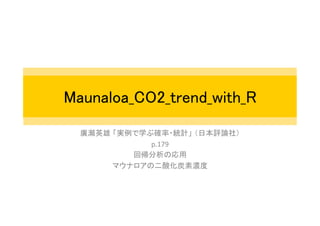