https://www.book4me.xyz/solution-manual-mechanics-of-flight-phillips/ Solution Manual for Mechanics of Flight - 2nd Edition Author(s) : Warren F. Phillips This solution manual include problems of all chapters of textbook (1 to 11)

1. W. F. Phillips, Mechanics of Flight, Second Edition: Solutions Manual by W. F. Phillips and N. R. Alley
Copyright © 2010 by John Wiley & Sons, Inc. 1 All rights reserved.
Chapter 1
Overview of Aerodynamics
1.1. The given data are a tabulation of the section lift, drag, and quarter-chord moment coefficients taken from test
data for a particular airfoil section. On one graph, plot both the section lift coefficient and the section normal
force coefficient as a function of angle of attack. On another graph, plot both the section drag coefficient and
the section axial force coefficient as a function of angle of attack.
Solution. The normal and axial force coefficients are found from
αα sin
~
cos
~~
DLN CCC += αα sin
~
cos
~~
LDA CCC −=
Using these equations in a spread-sheet gives
α (degs) LC
~
DC
~
4/
~
cmC NC
~
AC
~
−6.0 −0.38 0.0077 −0.0446 −0.37872 −0.032063
−5.0 −0.28 0.0071 −0.0440 −0.27955 −0.017331
−4.0 −0.18 0.0066 −0.0434 −0.18002 −0.005972
−3.0 −0.07 0.0063 −0.0428 −0.07023 0.002628
−2.0 0.04 0.0060 −0.0422 0.03977 0.007392
−1.0 0.14 0.0059 −0.0416 0.13988 0.008342
0.0 0.24 0.0058 −0.0410 0.24000 0.005800
1.0 0.35 0.0058 −0.0404 0.35005 −0.000309
2.0 0.46 0.0060 −0.0398 0.45993 −0.010057
3.0 0.56 0.0062 −0.0392 0.55956 −0.023117
4.0 0.65 0.0066 −0.0386 0.64888 −0.038758
5.0 0.76 0.0070 −0.0380 0.75772 −0.059265
6.0 0.87 0.0075 −0.0374 0.86602 −0.083481
7.0 0.97 0.0081 −0.0368 0.96376 −0.110174
8.0 1.07 0.0088 −0.0362 1.06081 −0.140201
9.0 1.16 0.0096 −0.0356 1.14722 −0.171982
10.0 1.26 0.0105 −0.0350 1.24268 −0.208456
11.0 1.35 0.0115 −0.0344 1.32739 −0.246303
12.0 1.44 0.0126 −0.0338 1.41115 −0.287068
Angle of Attack (degrees)
-6 -4 -2 0 2 4 6 8 10 12
-0.50
-0.25
0.00
0.25
0.50
0.75
1.00
1.25
1.50
-0.30
-0.25
-0.20
-0.15
-0.10
-0.05
0.00
0.05
CL
~
CN
~
CL
~
CN
~
CD
~
CA
~CA
~
CD
~
Notice that there is little difference between the lift and normal force coefficients but the difference between
the drag and axial force coefficients is large.
Access full Solution Manual only here
http://www.book4me.xyz/solution-manual-mechanics-of-flight-phillips/

2. W. F. Phillips, Mechanics of Flight, Second Edition: Solutions Manual by W. F. Phillips and N. R. Alley
Copyright © 2010 by John Wiley & Sons, Inc. 2 All rights reserved.
1.2. From the data presented in problem 1.1, on one graph, plot the location of the center of pressure, ,cxcp and
the aerodynamic center, ,cxac as a function of angle of attack.
Solution. The center of pressure is found from
N
m
N
mcp
C
C
C
C
c
x
c
x cx
~
~
25.0~
~
4/
−=−=
Using a central difference approximation for the aerodynamic derivatives, the aerodynamic center is found
from
)(
~
)(
~
)(
~
)(
~
25.0
2
)(
~
)(
~
2
)(
~
)(
~
25.0~
~
25.0~
~
4/4/
4/4/4/
,
,
,
,
αΔααΔα
αΔααΔα
αΔ
αΔααΔα
αΔ
αΔααΔα
α
α
α
α
−−+
−−+
−=
−−+−−+
−≅−=−=
NN
mm
NNmm
N
m
N
mac
CC
CC
CCCC
C
C
C
C
c
x
c
x
cc
cccx
Using these equations in a spread-sheet gives
α (degs) LC
~
DC
~
4/
~
cmC NC
~
cxcp cxac
-6.0 -0.38 0.0077 -0.0446 -0.37872 0.13224
-5.0 -0.28 0.0071 -0.0440 -0.27955 0.09261 0.24396
-4.0 -0.18 0.0066 -0.0434 -0.18002 0.00892 0.24427
-3.0 -0.07 0.0063 -0.0428 -0.07023 -0.35939 0.24454
-2.0 0.04 0.0060 -0.0422 0.03977 1.31120 0.24429
-1.0 0.14 0.0059 -0.0416 0.13988 0.54741 0.24401
0.0 0.24 0.0058 -0.0410 0.24000 0.42083 0.24429
1.0 0.35 0.0058 -0.0404 0.35005 0.36541 0.24454
2.0 0.46 0.0060 -0.0398 0.45993 0.33654 0.24427
3.0 0.56 0.0062 -0.0392 0.55956 0.32006 0.24365
4.0 0.65 0.0066 -0.0386 0.64888 0.30949 0.24394
5.0 0.76 0.0070 -0.0380 0.75772 0.30015 0.24447
6.0 0.87 0.0075 -0.0374 0.86602 0.29319 0.24418
7.0 0.97 0.0081 -0.0368 0.96376 0.28818 0.24384
8.0 1.07 0.0088 -0.0362 1.06081 0.28412 0.24346
9.0 1.16 0.0096 -0.0356 1.14722 0.28103 0.24340
10.0 1.26 0.0105 -0.0350 1.24268 0.27816 0.24334
11.0 1.35 0.0115 -0.0344 1.32739 0.27592 0.24288
12.0 1.44 0.0126 -0.0338 1.41115 0.27395
Angle of Attack (degrees)
-6 -4 -2 0 2 4 6 8 10 12
x/c
-1.50
-1.25
-1.00
-0.75
-0.50
-0.25
0.00
0.25
0.50
0.75
1.00
1.25
1.50
xcp/c
xac/c
xcp/c

3. W. F. Phillips, Mechanics of Flight, Second Edition: Solutions Manual by W. F. Phillips and N. R. Alley
Copyright © 2010 by John Wiley & Sons, Inc. 3 All rights reserved.
1.3. As predicted from thin airfoil theory, the section lift and leading-edge moment coefficients for a NACA 2412
airfoil section are given by
)03625.0(2
~
+= απLC and )07007.0(
2
~
+−= απ
lemC
where α is in radians. On one graph, plot both the section lift and normal force coefficients as a function of
angle of attack, from −6 to +12 degrees. On another graph, plot both the section drag and axial force
coefficients as a function of angle of attack, from −6 to +12 degrees.
Solution. Thin airfoil theory predicts zero drag and the normal and axial force coefficients are found from
ααπαα cos)03625.0(2sin
~
cos
~~
+=+= DLN CCC
ααπαα sin)03625.0(2sin
~
cos
~~
+−=−= LDA CCC
Using these equations in a spread-sheet gives
α (degs) α (rad) LC
~
DC
~
NC
~
AC
~
−6.0 −0.10472 −0.43021 0.000000 −0.42785 −0.044969
−5.0 −0.08727 −0.32055 0.000000 −0.31933 −0.027937
−4.0 −0.06981 −0.21088 0.000000 −0.21037 −0.014710
−3.0 −0.05236 −0.10122 0.000000 −0.10108 −0.005298
−2.0 −0.03491 0.00844 0.000000 0.00844 0.000295
−1.0 −0.01745 0.11810 0.000000 0.11809 0.002061
0.0 0.00000 0.22777 0.000000 0.22777 0.000000
1.0 0.01745 0.33743 0.000000 0.33738 −0.005889
2.0 0.03491 0.44709 0.000000 0.44682 −0.015603
3.0 0.05236 0.55675 0.000000 0.55599 −0.029138
4.0 0.06981 0.66641 0.000000 0.66479 −0.046487
5.0 0.08727 0.77608 0.000000 0.77312 −0.067640
6.0 0.10472 0.88574 0.000000 0.88089 −0.092585
7.0 0.12217 0.99540 0.000000 0.98798 −0.121309
8.0 0.13963 1.10506 0.000000 1.09431 −0.153795
9.0 0.15708 1.21473 0.000000 1.19977 −0.190025
10.0 0.17453 1.32439 0.000000 1.30427 −0.229978
11.0 0.19199 1.43405 0.000000 1.40770 −0.273630
12.0 0.20944 1.54371 0.000000 1.50998 −0.320956
Angle of Attack (degrees)
-6 -4 -2 0 2 4 6 8 10 12
-0.50
-0.25
0.00
0.25
0.50
0.75
1.00
1.25
1.50
-0.30
-0.25
-0.20
-0.15
-0.10
-0.05
0.00
0.05
CL
~
CN
~
CL
~
CN
~
CD
~
CA
~
CA
~
CD
~

4. W. F. Phillips, Mechanics of Flight, Second Edition: Solutions Manual by W. F. Phillips and N. R. Alley
Copyright © 2010 by John Wiley & Sons, Inc. 4 All rights reserved.
1.4. From the thin airfoil relations for the airfoil section presented in problem 1.3, on one graph, plot the location
of the center of pressure, ,cxcp and the aerodynamic center, ,cxac as a function of angle of attack, from −6
to +12 degrees.
Solution. From problem 1.3
)03625.0(2
~
+= απLC and )07007.0(
2
~
+−= απ
lemC
ααπαα cos)03625.0(2sin
~
cos
~~
+=+= DLN CCC
The center of pressure is found from
αα
α
ααπ
απ
cos)03625.0(4
)07007.0(
cos)03625.0(2
)07007.0)(2(
~
~
0.0~
~
+
+
=
+
+−
−=−=−=
N
m
N
mcp
C
C
C
C
c
x
c
x lex
The aerodynamic center is found from
]sin)03625.0([cos4
1
sin)03625.0(2cos2
)2(
~
~
0.0~
~
,
,
,
,
αααααπαπ
π
α
α
α
α
+−
=
+−
−
−=−=−=
N
m
N
mac
C
C
C
C
c
x
c
x lex
Using these equations in a spread-sheet gives
α (degs) α (rad) cxcp cxac
-6.00 -0.10472 0.12721 0.25320
-5.00 -0.08727 0.08459 0.25208
-4.00 -0.06981 -0.00192 0.25120
-3.00 -0.05236 -0.27521 0.25055
-2.00 -0.03491 6.54765 0.25014
-1.00 -0.01745 0.69992 0.24996
0.00 0.00000 0.48324 0.25000
1.00 0.01745 0.40750 0.25027
2.00 0.03491 0.36905 0.25078
3.00 0.05236 0.34589 0.25151
4.00 0.06981 0.33052 0.25248
. . . .
. . . .. . . .
10.00 0.17453 0.29459 0.26366
11.00 0.19199 0.29242 0.26650
12.00 0.20944 0.29077 0.26967
Angle of Attack (degrees)
-6 -4 -2 0 2 4 6 8 10 12
x/c
-1.50
-1.25
-1.00
-0.75
-0.50
-0.25
0.00
0.25
0.50
0.75
1.00
1.25
1.50
xcp/c
xac/c
xcp/c

5. W. F. Phillips, Mechanics of Flight, Second Edition: Solutions Manual by W. F. Phillips and N. R. Alley
Copyright © 2010 by John Wiley & Sons, Inc. 5 All rights reserved.
1.5. Write a computer subroutine to compute the geopotential altitude, temperature, pressure, and air density as a
function of geometric altitude for the standard atmosphere that is defined in Table 1.2.1. The only input
variable should be the geometric altitude in meters. All output variables should be in standard SI units. Test
this subroutine by comparing its output with the results that were obtained in Example 1.2.1 and those
presented in Appendix A.
Solution. The following Fortran subroutine provides one possible solution. Beyond 79,000 m this subroutine
assumes constant temperature, which is not according to the actual definition beyond 90,000 m.
Subroutine statsi(h,z,t,p,d)
! h = geometric altitude, specified by user (m)
! z = geopotential altitude, returned by subroutine (m)
! t = temperature, returned by subroutine (K)
! p = pressure, returned by subroutine (N/m**2)
! d = density, returned by subroutine (kg/m**3)
real Lt,zsa(0:8),Tsa(0:8),Psa(0:8)
data zsa/ 0.,11000.,20000.,32000.,47000.,52000.,61000.,79000.,9.9e20/
data Tsa/288.15,216.65,216.65,228.65,270.65,270.65,252.65,180.65,180.65/
data g0,R,Re,Psa(0)/9.80665,287.0528,6356766.,101325./
z=Re*h/(Re+h)
do i=1,8
Lt=-(Tsa(i)-Tsa(i-1))/(zsa(i)-zsa(i-1))
if(Lt.eq.0.)then
if(z.le.zsa(i))then
t=Tsa(i-1)
p=Psa(i-1)*exp(-g0*(z-zsa(i-1))/R/Tsa(i-1))
d=p/R/t
return
else
Psa(i)=Psa(i-1)*exp(-g0*(zsa(i)-zsa(i-1))/R/Tsa(i-1))
endif
else
ex=g0/R/Lt
if(z.lt.zsa(i))then
t=Tsa(i-1)-Lt*(z-zsa(i-1))
p=Psa(i-1)*(t/Tsa(i-1))**ex
d=p/R/t
return
else
Psa(i)=Psa(i-1)*(Tsa(i)/Tsa(i-1))**ex
endif
endif
end do
t=Tsa(8)
p=0.0
d=0.0
return
end
http://www.book4me.xyz/solution-manual-mechanics-of-flight-phillips/

6. W. F. Phillips, Mechanics of Flight, Second Edition: Solutions Manual by W. F. Phillips and N. R. Alley
Copyright © 2010 by John Wiley & Sons, Inc. 6 All rights reserved.
1.6. Write a computer subroutine to compute the geopotential altitude, temperature, pressure, and air density as a
function of geometric altitude for the standard atmosphere that is defined in Table 1.2.1. The only input
variable should be the geometric altitude in feet. All output variables should be in English engineering units.
Test the subroutine by comparison with Example 1.2.2 and the results presented in Appendix B. Since this
standard atmosphere is defined in SI units, this subroutine could be written using simple unit conversion and
a single call to the subroutine written for problem 1.5.
Solution. The following Fortran subroutine provides one possible solution.
Subroutine statee(h,z,t,p,d)
c h = geometric altitude, specified by user (ft)
c z = geopotential altitude, returned by subroutine (ft)
c t = temperature, returned by subroutine (R)
c p = pressure, returned by subroutine (lbf/ft**2)
c d = density, returned by subroutine (slugs/ft**3)
hsi=h*0.3048
call statsi(hsi,zsi,tsi,psi,dsi)
z=zsi/0.3048
t=tsi*1.8
p=psi*0.02088543
d=dsi*0.001940320
return
end
1.7. Show that the velocity distribution for the 2-D source flow, which is expressed in Eq. (1.5.4), is irrotational.
Solution. For this flow
r
r
iV
π
Λ
2
=
In cylindrical coordinates the vorticity is given by
0
00
2
1111
=
∂
∂
∂
∂
∂
∂
=
∂
∂
∂
∂
∂
∂
=×∇
r
zr
rr
VrVV
zr
rr
zr
zr
zr
π
Λ
θθ
θ
θ
θ iiiiii
V
1.8. Show that the velocity distribution for the 2-D vortex flow, which is expressed in Eq. (1.5.6), is irrotational.
Solution. For this flow
θ
π
Γ iV
r2
−=
In cylindrical coordinates the vorticity is given by
0
0
2
0
1111
=
−
∂
∂
∂
∂
∂
∂
=
∂
∂
∂
∂
∂
∂
=×∇
π
Γ
θθ
θ
θ
θ
zr
rr
VrVV
zr
rr
zr
zr
zr iiiiii
V

7. W. F. Phillips, Mechanics of Flight, Second Edition: Solutions Manual by W. F. Phillips and N. R. Alley
Copyright © 2010 by John Wiley & Sons, Inc. 7 All rights reserved.
1.9. Show that the velocity distribution for the 2-D doublet flow, which is expressed in Eq. (1.5.8), is irrotational.
Solution. For this flow
θ
π
θκ
π
θκ iiV 22
2
sin
2
cos
rr
r −−=
In cylindrical coordinates the vorticity is given by
01
2
sin
2
sin
0
2
sin
2
cos
1111
22
2
=
⎟
⎟
⎠
⎞
⎜
⎜
⎝
⎛
−=
−−
∂
∂
∂
∂
∂
∂
=
∂
∂
∂
∂
∂
∂
=×∇ z
zr
zr
zr
rrr
rr
zr
rr
VrVV
zr
rr
i
iiiiii
V
π
θκ
π
θκ
π
θκ
π
θκ
θθ
θ
θ
θ
1.10. Show that the velocity distribution for the 2-D stagnation flow, which is expressed in Eq. (1.5.10), is
irrotational.
Solution. For this flow
yx ByBx iiV −=
In Cartesian coordinates the vorticity is given by
0
0
=
−
∂
∂
∂
∂
∂
∂
=
∂
∂
∂
∂
∂
∂
=×∇
ByBx
zyx
VVV
zyx
zyx
zyx
zyx iiiiii
V
1.11. Show that the velocity distribution for the 2-D vortex flow, which is expressed in Eq. (1.5.6), satisfies the
incompressible continuity equation.
Solution. For this flow
θ
π
Γ iV
r2
−=
The incompressible continuity equation is given by
0=⋅∇ V
In cylindrical coordinates the divergence is given by
( ) ( ) ( ) ( ) ( ) 00
2
10111 =
∂
∂
+⎟
⎠
⎞
⎜
⎝
⎛
−
∂
∂
+
∂
∂
=
∂
∂
+
∂
∂
+
∂
∂
=⋅∇
zrrrr
V
z
V
r
rV
rr
zr
π
Γ
θθ
θV

8. W. F. Phillips, Mechanics of Flight, Second Edition: Solutions Manual by W. F. Phillips and N. R. Alley
Copyright © 2010 by John Wiley & Sons, Inc. 8 All rights reserved.
1.12. The section geometry for a NACA 4-digit series airfoil is completely fixed by the maximum camber, the
location of maximum camber, the maximum thickness, and the chord length. The first digit indicates the
maximum camber in percent of chord. The second digit indicates the distance from the leading edge to the
point of maximum camber in tenths of the chord. The last two digits indicate the maximum thickness in
percent of chord. The camber line is given by
⎪
⎪
⎩
⎪
⎪
⎨
⎧
≤≤
⎥
⎥
⎦
⎤
⎢
⎢
⎣
⎡
⎟
⎠
⎞
⎜
⎝
⎛
−
−−⎟
⎠
⎞
⎜
⎝
⎛
−
−
≤≤
⎥
⎥
⎦
⎤
⎢
⎢
⎣
⎡
⎟
⎠
⎞
⎜
⎝
⎛
−⎟
⎠
⎞
⎜
⎝
⎛
=
cxx
xc
xc
xc
xcy
xx
x
x
x
xy
xy
mc
mcmc
mc
mc
mcmc
mc
c
,2
0,2
)( 2
2
where ymc is the maximum camber and xmc is the position of maximum camber. The thickness about the
camber line, measured perpendicular to the camber line itself, is given by
⎥
⎥
⎦
⎤
⎢
⎢
⎣
⎡
⎟
⎠
⎞
⎜
⎝
⎛−⎟
⎠
⎞
⎜
⎝
⎛+⎟
⎠
⎞
⎜
⎝
⎛−⎟
⎠
⎞
⎜
⎝
⎛−=
432
015.1843.2516.3260.1969.2)(
c
x
c
x
c
x
c
x
c
xtxt m
where tm is the maximum thickness. For the NACA 2412 airfoil section, determine x/c and y/c for the camber
line, upper surface, and lower surface at chordwise positions of x/c = 0.10.
Solution. The NACA 2412 airfoil section has 2% maximum camber located at 40% chord. We wish to
determine the dimensionless coordinates of the camber line at 10% chord. Thus, we use the camber line
definition for mcxx ≤≤0 , which gives
10.0==
c
x
c
xc
00875.0
40.0
10.0
40.0
10.0202.02
22
=⎥
⎦
⎤
⎢
⎣
⎡
⎟
⎠
⎞
⎜
⎝
⎛−⎟
⎠
⎞
⎜
⎝
⎛=
⎥
⎥
⎦
⎤
⎢
⎢
⎣
⎡
⎟
⎠
⎞
⎜
⎝
⎛
−⎟
⎠
⎞
⎜
⎝
⎛
=
cx
cx
cx
cx
c
y
c
y
mcmc
mcc
Similarly, the dimensionless thickness at 10% chord is
( ) ( ) ( ) ( )[ ]
0936554.0
1.0015.11.0843.21.0516.31.0260.11.0969.212.0
015.1843.2516.3260.1969.2
432
432
=
−+−−=
⎥
⎦
⎤
⎢
⎣
⎡
⎟
⎠
⎞
⎜
⎝
⎛−⎟
⎠
⎞
⎜
⎝
⎛+⎟
⎠
⎞
⎜
⎝
⎛−⎟
⎠
⎞
⎜
⎝
⎛−=
c
x
c
x
c
x
c
x
c
x
c
t
c
t m
From the camber line definition, the camber line slope at 10% chord is
075.0
40.0
10.01
40.0
02.0212212 2
=⎥⎦
⎤
⎢⎣
⎡
⎟
⎠
⎞
⎜
⎝
⎛−=⎥
⎦
⎤
⎢
⎣
⎡
⎟
⎠
⎞
⎜
⎝
⎛
−=⎥
⎦
⎤
⎢
⎣
⎡
⎟⎟
⎠
⎞
⎜⎜
⎝
⎛
−⎟
⎠
⎞
⎜
⎝
⎛
=
cx
cx
cx
cy
x
x
x
y
dx
dy
mcmc
mc
mcmc
mc
c
Using Eqs. (1.6.1) through (1.6.4), the dimensionless coordinates of the upper and lower surfaces at 10%
chord are

9. W. F. Phillips, Mechanics of Flight, Second Edition: Solutions Manual by W. F. Phillips and N. R. Alley
Copyright © 2010 by John Wiley & Sons, Inc. 9 All rights reserved.
( ) ( )
096498.0075.0
075.012
0936554.010.0
12 22
=
+
−=
+
−=
dx
dy
dxdy
ct
c
x
c
x c
c
u
( ) ( )
055447.0
075.012
0936554.000875.0
12 22
=
+
+=
+
+=
dxdy
ct
c
y
c
y
c
cu
( ) ( )
103502.0075.0
075.012
0936554.010.0
12 22
=
+
+=
+
+=
dx
dy
dxdy
ct
c
x
c
x c
c
l
( ) ( )
037947.0
075.012
0936554.000875.0
12 22
−=
+
−=
+
−=
dxdy
ct
c
y
c
y
c
cl
1.13. Using the formulas given in problem 1.12, for the NACA 0012 airfoil section, determine x/c and y/c of the
upper and lower surfaces at chordwise positions of x/c = 0.00, 0.001, 0.10, 0.40, 0.50, 0.90, and 1.00.
Solution. Following the procedure used in the solution to problem 1.12 results in
xc yc xu yu xl yl
0.000000 0.000000 0.000000 0.000000 0.000000 0.000000
0.001000 0.000000 0.001000 0.005557 0.001000 −0.005557
0.100000 0.000000 0.100000 0.046828 0.100000 −0.046828
0.400000 0.000000 0.400000 0.058030 0.400000 −0.058030
0.500000 0.000000 0.500000 0.052940 0.500000 −0.052940
0.900000 0.000000 0.900000 0.014477 0.900000 −0.014477
1.000000 0.000000 1.000000 0.001260 1.000000 −0.001260
1.14. Using the formulas given in problem 1.12, for the NACA 4421 airfoil section, determine x/c and y/c of the
upper and lower surfaces at chordwise positions of x/c = 0.00, 0.001, 0.10, 0.40, 0.50, 0.90, and 1.00.
Solution. Following the procedure used in the solution to problem 1.12 results in
xc yc xu yu xl yl
0.000000 0.000000 0.000000 0.000000 0.000000 0.000000
0.001000 0.000200 −0.000903 0.009737 0.002903 −0.009338
0.100000 0.017500 0.087844 0.098542 0.112156 −0.063542
0.400000 0.040000 0.400000 0.141553 0.400000 −0.061553
0.500000 0.038889 0.502058 0.131511 0.497942 −0.053734
0.900000 0.012222 0.902798 0.037402 0.897202 −0.012958
1.000000 0.000000 1.000291 0.002186 0.999709 −0.002186

10. W. F. Phillips, Mechanics of Flight, Second Edition: Solutions Manual by W. F. Phillips and N. R. Alley
Copyright © 2010 by John Wiley & Sons, Inc. 10 All rights reserved.
1.15. Using the formulas given in problem 1.12, for the NACA 0021 airfoil section, determine the angle of the
upper surface relative to the chord line in degrees at a chordwise position of x/c = 0.10.
Solution. The slope of the upper surface is
dx
dx
dx
dy
dx
dy uu
u
u
= (1)
From Eqs. (1.6.1) and (1.6.2), for this symmetric airfoil with yc = 0 we have
( )
1
12 2
==
⎥
⎥
⎦
⎤
⎢
⎢
⎣
⎡
+
−=
dx
dx
dx
dy
dxdy
tx
dx
d
dx
dx c
c
u
(2)
( ) dx
dt
dxdy
ty
dx
d
dx
dy
c
c
u
2
1
12 2
=
⎥
⎥
⎦
⎤
⎢
⎢
⎣
⎡
+
+= (3)
From the thickness definition in problem 1.12, with x/c = 0.1 and tm/c = 0.21
( ) ( ) 59061.01.0)015.1(41.0)843.2(31.0)516.3(2260.1
1.0
1
2
969.221.0
)015.1(4)843.2(3)516.3(2260.11
2
969.2
015.1843.2516.3260.1969.2
32
32
432
=⎥
⎦
⎤
⎢
⎣
⎡
−+−−=
⎥
⎥
⎦
⎤
⎢
⎢
⎣
⎡
⎟
⎠
⎞
⎜
⎝
⎛−⎟
⎠
⎞
⎜
⎝
⎛+−−=
⎥
⎥
⎦
⎤
⎢
⎢
⎣
⎡
⎟
⎠
⎞
⎜
⎝
⎛−⎟
⎠
⎞
⎜
⎝
⎛+⎟
⎠
⎞
⎜
⎝
⎛−⎟
⎠
⎞
⎜
⎝
⎛−=
c
x
c
x
c
x
cxc
t
c
x
c
x
c
x
c
x
c
x
dx
d
t
dx
dt
m
m
Using Eqs. (2) and (3) in Eq. (1) gives
dx
dt
dx
dy
u
u
2
1=
and
°==⎟
⎠
⎞
⎜
⎝
⎛=⎟
⎠
⎞
⎜
⎝
⎛=⎟
⎠
⎞
⎜
⎝
⎛
= −−−
45.1628714.0
2
59061.0tan
2
1tantan 111
dx
dt
dx
dy
u
u
uθ
1.16. Using the formulas given in problem 1.12, for the NACA 4421 airfoil section, determine the angle of the
upper surface relative to the chord line in degrees at a chordwise position of x/c = 0.10.
Solution. The slope of the upper surface is
dx
dx
dx
dy
dx
dy uu
u
u
= (1)
From Eqs. (1.6.1) and (1.6.2), for this cambered airfoil we have
http://www.book4me.xyz/solution-manual-mechanics-of-flight-phillips/

11. W. F. Phillips, Mechanics of Flight, Second Edition: Solutions Manual by W. F. Phillips and N. R. Alley
Copyright © 2010 by John Wiley & Sons, Inc. 11 All rights reserved.
( )
( ) ( )[ ]
( )
( ) ( )
( ) ⎥
⎥
⎦
⎤
⎢
⎢
⎣
⎡
+
−
−−+
+
=
⎟
⎠
⎞
⎜
⎝
⎛
+
+⎟
⎟
⎠
⎞
⎜
⎜
⎝
⎛
+
+
−=
⎥
⎥
⎦
⎤
⎢
⎢
⎣
⎡
+
−
∂
∂
=
∂
∂
2
2
2
2
2
2
2
22
2322
2
2
2
1
1
12
12
1
2
122
1
12
11
12
dx
yd
t
dxdy
dxdy
dx
dt
dx
dy
dxdy
dxdy
dx
yd
dx
dy
dxdy
t
dx
yd
t
dx
dt
dx
dy
dxdy
dx
dy
dxdy
tx
xx
x
c
c
cc
c
c
cc
c
cc
c
c
c
u
(2)
( ) ( ) ( )[ ]
( )
( )
( ) ⎥
⎥
⎦
⎤
⎢
⎢
⎣
⎡
∂
∂
+
−
∂
∂++
∂
∂
+
=
∂
∂
∂
∂
+
−
∂
∂
+
+
∂
∂
=
⎥
⎥
⎦
⎤
⎢
⎢
⎣
⎡
+
+
∂
∂
=
∂
∂
2
2
2
2
2
2
2
23222
1
12
12
1
2
122
1
12
1
12
x
y
t
dxdy
dxdy
x
tdxdy
x
y
dxdy
x
y
x
y
dxdy
t
x
t
dxdyx
y
dxdy
ty
xx
y
c
c
c
c
c
c
cc
cc
c
c
c
u
(3)
From the camber line definition in problem 1.12, with x/c = 0.1, xmc/c = 0.4, and ymc/c = 0.04
15.0
4.0
1.01
4.0
04.0212222
2
=⎟
⎠
⎞
⎜
⎝
⎛ −=⎟
⎠
⎞
⎜
⎝
⎛
−=⎟
⎠
⎞
⎜
⎝
⎛
−=
⎥
⎥
⎦
⎤
⎢
⎢
⎣
⎡
⎟
⎠
⎞
⎜
⎝
⎛
−⎟
⎠
⎞
⎜
⎝
⎛
=
cx
cx
cx
cy
x
x
x
y
x
x
x
x
dx
d
y
dx
dy
mcmc
mc
mcmc
mc
mcmc
mc
c
ccccx
cy
x
y
x
x
x
x
dx
d
y
dx
yd
mc
mc
mc
mc
mcmc
mc
c 15.01
)4.0(
04.021
)(
222 222
2
2
2
2
2
−=−=−=−=
⎥
⎥
⎦
⎤
⎢
⎢
⎣
⎡
⎟
⎠
⎞
⎜
⎝
⎛
−⎟
⎠
⎞
⎜
⎝
⎛
=
From the thickness definition in problem 1.12, with x/c = 0.1 and tm/c = 0.21
cc
c
x
c
x
c
x
c
x
c
x
c
t
t m
16390.0015.1843.2516.3260.1969.2
432
=
⎥
⎥
⎦
⎤
⎢
⎢
⎣
⎡
⎟
⎠
⎞
⎜
⎝
⎛−⎟
⎠
⎞
⎜
⎝
⎛+⎟
⎠
⎞
⎜
⎝
⎛−⎟
⎠
⎞
⎜
⎝
⎛−=
59061.0)015.1(4)843.2(3)516.3(2260.11
2
969.2
32
=
⎥
⎥
⎦
⎤
⎢
⎢
⎣
⎡
⎟
⎠
⎞
⎜
⎝
⎛−⎟
⎠
⎞
⎜
⎝
⎛+−−=
c
x
c
x
c
x
cxc
t
dx
dt m
Using Eqs. (2) and (3) in Eq. (1) gives
( )
( )
( ) ( )
( )
45026.0
1
1
12
1
12
2
2
2
2
2
2
2
2
2
=
+
−
−−+
∂
∂
+
−
∂
∂++
∂
∂
=
dx
yd
t
dxdy
dxdy
dx
dt
dx
dy
dxdy
x
y
t
dxdy
dxdy
x
tdxdy
x
y
dx
dy
c
c
cc
c
c
c
c
c
c
u
u
( ) °===⎟
⎠
⎞
⎜
⎝
⎛
= −−
24.2442307.045026.0tantan 11
u
u
u
dx
dy
θ
This can be closely approximated as
°==⎟
⎠
⎞
⎜
⎝
⎛ +=⎟
⎠
⎞
⎜
⎝
⎛
+≅ −−
00.2441984.015.0
2
59061.0tan
2
1tan 11
dx
dy
dx
dt c
uθ

12. W. F. Phillips, Mechanics of Flight, Second Edition: Solutions Manual by W. F. Phillips and N. R. Alley
Copyright © 2010 by John Wiley & Sons, Inc. 12 All rights reserved.
1.17. The formulas for the geometry of a NACA 4-digit series airfoil are given in problem 1.12. For the NACA
2412 airfoil section, use thin airfoil theory to determine the zero-lift angle of attack, the lift coefficients at 0-
and 5-degree angles of attack, and the quarter-chord moment coefficient. Also plot the center of pressure as a
function of angle of attack from −5 to 10 degrees.
Solution. From the camber line definition in problem 1.12, with xmc/c = 0.4 and ymc/c = 0.02
⎪
⎪
⎩
⎪⎪
⎨
⎧
≤≤⎟
⎠
⎞
⎜
⎝
⎛ −−⎟
⎠
⎞
⎜
⎝
⎛ −
≤≤⎟
⎠
⎞
⎜
⎝
⎛−⎟
⎠
⎞
⎜
⎝
⎛
=
0.14.0,1
18
11
15
1
4.00.0,
8
1
10
1
2
2
c
x
c
x
c
x
c
x
c
x
c
x
c
yc
Differentiating the given camber line equation, the camber line slope is
⎪
⎩
⎪
⎨
⎧
≤≤−
≤≤−
=
0.14.0,
9
1
45
2
4.00.0,
4
1
10
1
c
x
c
x
c
x
c
x
dx
dyc
Using the change of variables
)cos1(
2
1 θ−≡
c
x
we have
⎪
⎩
⎪
⎨
⎧
≤−≤−−
≤−≤−−
=
0.2)cos1(8.0,)cos1(
18
1
45
2
8.0)cos1(0.0,)cos1(
8
1
10
1
θθ
θθ
dx
dyc
From the definition of θ, we can write
⎟
⎠
⎞
⎜
⎝
⎛ −≡ −
c
x21cos 1
θ
( ) 1.36943848.01cos21cos 11
=−=⎟
⎠
⎞
⎜
⎝
⎛
−= −−
c
xmc
mcθ
⎪
⎩
⎪
⎨
⎧
≤≤−
≤≤−
=
πθθ
θθ
1.3694384,
90
1cos
18
1
1.36943840,
40
1cos
8
1
dx
dyc
The first three coefficients in the series solution are then
⎥
⎥
⎦
⎤
⎢
⎢
⎣
⎡
⎟
⎠
⎞
⎜
⎝
⎛ −+⎟
⎠
⎞
⎜
⎝
⎛ −−=−= ∫∫∫
=
θθθθ
π
αθ
π
α
ππ
θ
ddd
dx
dy
A c
1.3694384
1.3694384
00
0
90
1cos
18
1
40
1cos
8
111
⎥
⎥
⎦
⎤
⎢
⎢
⎣
⎡
⎟
⎠
⎞
⎜
⎝
⎛ −+⎟
⎠
⎞
⎜
⎝
⎛ −−=
π
θθθθ
π
α
1.3694384
1.3694384
0 9018
sin
408
sin1
⎥
⎦
⎤
⎢
⎣
⎡
+−−−−=
90
1.3694384
18
384)sin(1.3694
9040
1.3694384
8
384)sin(1.36941 π
π
α
60.00449288−= α

13. W. F. Phillips, Mechanics of Flight, Second Edition: Solutions Manual by W. F. Phillips and N. R. Alley
Copyright © 2010 by John Wiley & Sons, Inc. 13 All rights reserved.
θθ
π
π
θ
d
dx
dy
A c
cos2
0
1 ∫
=
=
⎥
⎥
⎦
⎤
⎢
⎢
⎣
⎡
⎟⎟
⎠
⎞
⎜⎜
⎝
⎛
−+⎟⎟
⎠
⎞
⎜⎜
⎝
⎛
−= ∫∫ θθθθθθ
π
π
dd
1.3694384
21.3694384
0
2
90
cos
18
cos
40
cos
8
cos2
⎥
⎥
⎦
⎤
⎢
⎢
⎣
⎡
⎟
⎠
⎞
⎜
⎝
⎛ −++⎟
⎠
⎞
⎜
⎝
⎛ −+=
π
θθθθθθθθ
π 1.3694384
1.3694384
0 90
sin
36
cossin
40
sin
16
cossin2
⎥
⎦
⎤
+
+
−+
⎢
⎣
⎡
−
+
=
90
384)sin(1.3694
36
1.3694384384)cos(1.3694384)sin(1.3694
36
40
384)sin(1.3694
16
1.3694384384)cos(1.3694384)sin(1.36942
π
π
0.08149514=
θθ
π
π
θ
d
dx
dy
A c
)2cos(2
0
2 ∫
=
=
⎥
⎥
⎦
⎤
⎢
⎢
⎣
⎡
⎟
⎠
⎞
⎜
⎝
⎛ −+⎟
⎠
⎞
⎜
⎝
⎛ −= ∫∫ θθθθθθ
π
π
dd
1.3694384
1.3694384
0
)2cos(
90
1cos
18
1)2cos(
40
1cos
8
12
⎥
⎥
⎦
⎤
⎢
⎢
⎣
⎡
−⎟
⎠
⎞
⎜
⎝
⎛ −+−⎟
⎠
⎞
⎜
⎝
⎛ −= ∫∫ θθθθθθ
π
π
dd
1.3694384
2
1.3694384
0
2
)1cos2(
90
1cos
18
1)1cos2(
40
1cos
8
12
⎥
⎥
⎦
⎤
⎟⎟
⎠
⎞
⎜⎜
⎝
⎛
+−−+
⎢
⎢
⎣
⎡
⎟⎟
⎠
⎞
⎜⎜
⎝
⎛
+−−=
∫
∫
θθθθ
θθθθ
π
π
d
d
1.3694384
23
1.3694384
0
23
90
1
18
cos
45
cos
9
cos
40
1
8
cos
20
cos
4
cos2
⎥
⎥
⎦
⎤
⎟
⎟
⎠
⎞
⎜
⎜
⎝
⎛
+−+−
+
+
⎢
⎢
⎣
⎡
⎟
⎟
⎠
⎞
⎜
⎜
⎝
⎛
+−+−
+
=
π
θθθθθθθ
θθθθθθθ
π
1.3694384
2
1.3694384
0
2
9018
sin
90
cossin
27
)2(cossin
408
sin
40
cossin
12
)2(cossin2
80.0138612
18
384)sin(1.3694
90
384)cos(1.3694384)sin(1.3694
27
]2)(1.3694384384)[cossin(1.3694
8
384)sin(1.3694
40
384)cos(1.3694384)sin(1.3694
12
]2)(1.3694384384)[cossin(1.36942
2
2
=⎥
⎦
⎤
++
+
−
−−
⎢
⎢
⎣
⎡ +
=
π
The section lift coefficient is
( ) ( )012
1
0 240.036254682)(2
~
LL AAC ααπαππ −=+=+=
Thus, the zero-lift angle of attack for this airfoil is

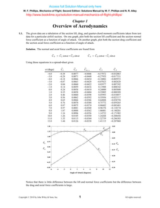
14. W. F. Phillips, Mechanics of Flight, Second Edition: Solutions Manual by W. F. Phillips and N. R. Alley
Copyright © 2010 by John Wiley & Sons, Inc. 14 All rights reserved.
°−=−= 2.077rad40.036254680Lα
The section lift coefficient at a 0-degree angle of attack is
( ) ( )[ ] 80.22740.03625468022
~
0 =−−=−= πααπ LLC
The section lift coefficient at a 5-degree angle of attack is
( ) ( )[ ] 0.776140.03625468180522
~
0 =−−=−= ππααπ LLC
The quarter-chord moment coefficient at any angle of attack is
( ) ( ) 0.053120.0814951480.0138612
44
~
124
−=−=−= ππ AAC cm
The center of pressure is determined from
( )
( )
( )
40.03625468
00845423250
4
1
4)]0.03625468([8
80.01386120.08149514
4
1
84
1
~
44
1
21
0
21
+
+=
−−
−+=
−
−
+=−+=
α
α
ααπ
ππ
.
AAAA
Cc
x
LL
cp
From this equation, the center of pressure as a function of angle of attack is shown in Fig. 1.17. Notice that,
for this cambered airfoil, the center of pressure moves dramatically with angle of attack, particularly in the
region near the zero lift angle of attack. The result shown in this figure is typical of center of pressure
variation with angle of attack for all cambered airfoils. For this reason, center of pressure is almost never
used when working with cambered airfoils. For symmetric airfoils, however, the center of pressure remains
fixed at the quarter-chord, independent of angle of attack.
Angle of Attack (degrees)
-5 0 5 10
x/c
-1.5
-1.0
-0.5
0.0
0.5
1.0
1.5
xcp/c
xac/c = 0.25
xcp/c
Figure 1.17 Variation in center of pressure with angle of attack for a NACA 2412 airfoil, as predicted by thin
airfoil theory.

15. W. F. Phillips, Mechanics of Flight, Second Edition: Solutions Manual by W. F. Phillips and N. R. Alley
Copyright © 2010 by John Wiley & Sons, Inc. 15 All rights reserved.
1.18. The formulas for the geometry of a NACA 4-digit series airfoil are given in problem 1.12. Using thin airfoil
theory, for the NACA 4412 airfoil section, determine the zero-lift angle of attack, the lift coefficients at 0-
and 5-degree angles of attack, the quarter-chord moment coefficient, and the center of pressure at the 0- and
5-degree angles of attack.
Solution. From the camber line definition in problem 1.12, with xmc/c = 0.4 and ymc/c = 0.04
⎪
⎪
⎩
⎪⎪
⎨
⎧
≤≤⎟
⎠
⎞
⎜
⎝
⎛ −−⎟
⎠
⎞
⎜
⎝
⎛ −
≤≤⎟
⎠
⎞
⎜
⎝
⎛−⎟
⎠
⎞
⎜
⎝
⎛
=
0.14.0,1
9
11
15
2
4.00.0,
4
1
5
1
2
2
c
x
c
x
c
x
c
x
c
x
c
x
c
yc
Differentiating the given camber line equation, the camber line slope is
⎪
⎩
⎪
⎨
⎧
≤≤−
≤≤−
=
0.14.0,
9
2
45
4
4.00.0,
2
1
5
1
c
x
c
x
c
x
c
x
dx
dyc
Using the change of variables
)cos1(
2
1 θ−≡
c
x
we have
⎪
⎩
⎪
⎨
⎧
≤−≤−−
≤−≤−−
=
0.2)cos1(8.0,)cos1(
9
1
45
4
8.0)cos1(0.0,)cos1(
4
1
5
1
θθ
θθ
dx
dyc
From the definition of θ, we can write
⎟
⎠
⎞
⎜
⎝
⎛ −≡ −
c
x21cos 1
θ
( ) 1.36943848.01cos21cos 11
=−=⎟
⎠
⎞
⎜
⎝
⎛
−= −−
c
xmc
mcθ
⎪
⎩
⎪
⎨
⎧
≤≤−
≤≤−
=
πθθ
θθ
1.3694384,
45
1cos
9
1
1.36943840,
20
1cos
4
1
dx
dyc
The first three coefficients in the series solution are then
⎥
⎥
⎦
⎤
⎢
⎢
⎣
⎡
⎟
⎠
⎞
⎜
⎝
⎛ −+⎟
⎠
⎞
⎜
⎝
⎛ −−=−= ∫∫∫
=
θθθθ
π
αθ
π
α
ππ
θ
ddd
dx
dy
A c
1.3694384
1.3694384
00
0
45
1cos
9
1
20
1cos
4
111
⎥
⎥
⎦
⎤
⎢
⎢
⎣
⎡
⎟
⎠
⎞
⎜
⎝
⎛ −+⎟
⎠
⎞
⎜
⎝
⎛ −−=
π
θθθθ
π
α
1.3694384
1.3694384
0 459
sin
204
sin1
⎥
⎦
⎤
⎢
⎣
⎡
+−−−−=
45
1.3694384
9
384)sin(1.3694
4520
1.3694384
4
384)sin(1.36941 π
π
α
8985770.00−= α
http://www.book4me.xyz/solution-manual-mechanics-of-flight-phillips/