Software Reliability models have been in existence since the early 1970, over 200 have been developed. Some of the older models have been discarded based upon more recent information about the assumptions, and newer ones have replaced them.

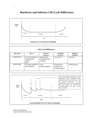
1. 1
Hilaire Ananda Perera
Long Term Quality Assurance
Hardware and Software Life Cycle Differences
Life Cycle Differences
Life Cycle Pre. t0 Period A
(t0 to t1)
Period B
(t1 to t2)
Period C
(Post t2)
HARDWARE  Concept Definition
 Development
 Build
Test
 Deployment
 Infant Mortality
 Upgrade
 Useful Life  Wearout
SOFTWARE  Concept Definition
 Development
 Test
 Debug/Upgrade
 Deployment
 Useful Life
 Debug/Upgrade
 Obsolescence
Failure
Rate
Timet0 t1 t2
Period A
Period B Period C
Bathtub Curve for Hardware Reliability
U
P
G
R
A
D
E
U
P
G
R
A
D
E
U
P
G
R
A
D
E
Revised Bathtub Curve for Software Reliability
Timet0 t1 t2
Failure
Rate
Period A Period B Period C
Since each upgrade represents a mini
development cycle, modifications may
introduce new defects in other parts of
the software unrelated to the
modification itself. The more upgrades
that occur, greater the potential for
increased failure rate, and hence
lower reliability

2. 2
Hilaire Ananda Perera
Long Term Quality Assurance
0
5
10
15
20
25
30
0.000 0.020 0.040 0.060 0.080 0.100 0.120
Fault Rate (n/t)
FaultNumber(n)
Fault Rate Plot
One goal of testing is to estimate N, the total (inherent) number of faults and fault density,
based upon observing an actual total of n faults during the testing period t. If the fault rate
value n/t is plotted at the occurrence of each fault, the resultant plot can be used to estimate
N under the assumption of a linear fault rate.
From the above plot, inherent number of faults N = 28
From the above plot, inherent fault (defect) density = 0.28 faults per KSLOC
Mean Time Between Failures
From the above table the Mean Time Between Failures (MTBF) can be calculated.
MTBF = (10 + 9 + ........... + 40) = 296/15 = 19.73
SOFTWARE FAILURE DATA
Time-Based Failure
100 KSLOC of Software
Failure
Number
Failure
Time
Failure
Interval
1 10 10
2 19 9
3 32 13
4 43 11
5 58 15
6 70 12
7 88 18
8 103 15
9 125 22
10 150 25
11 169 19
12 199 30
13 231 32
14 256 25
15 296 40
KSLOC = 1000 Source Lines Of Code

3. 3
Hilaire Ananda Perera
Long Term Quality Assurance
SOFTWARE RELIABILITY MODELS
Software reliability models have been in existence since the early 1970; over 200 have been
developed. Certainly some of the more recent ones build upon the theory and principles of
the older ones. Some of the older models have been discarded based upon more recent
information about the assumptions and newer ones have replaced them.
The general topic of software reliability modeling is divided into two major categories,
prediction and estimation.
ISSUES PREDICTION MODELS ESTIMATION MODELS
DATA
REFERENCE
Uses historical data Uses data from current software
development effort
WHEN USED IN
DEVELOPMENT
CYCLE
Usually made prior to development
or test phases; can be used as early
as concept phase
Usually made later in life cycle
(after some data have been
collected); not typically used in
concept or development phases
TIME
FRAME
Predict reliability at some future
time
Estimate reliability at either present
or some future time
Prediction Models
Four prediction models are available. Musa’s Execution Time Model (See Page 4), Putnam’s
Model, two models ( TR-92-51 Model, TR-92-15 Model) developed at Rome Laboratory.
Whenever possible, it is recommended that a prediction model be used.
Estimation Models
Estimation models have been classified into three major types which are test coverage,
tagging and fault counts. Test Coverage models assume that software reliability is a function
of the amount of software that has been successfully tested or verified. Tagging models
introduce faults into software and then track the number of these faults that are found during
testing in order to estimate the total number of faults. The fault count and/or fault rate
estimation models (General Exponential; Lloyd-Lipow; Musa’s Basic; Musa’s Logarithmic;
Shooman’s; Goel-Okumoto) either predict the number of faults detected during some time
interval or the time when a specific number of faults will be detected. One model may work
well (i.e. provide useful predictions/estimates) with a few data sets but then not be useful for
others. The future development of one universally accepted useful reliability model appears
to be unobtainable since the topic has been approached from so many different perspectives
with no overall success.

4. 4
Hilaire Ananda Perera
Long Term Quality Assurance
MUSA’S EXECUTION TIME MODEL
Developed by John Musa of Bell Laboratories in the mid 1970s, this was one of the earliest
reliability prediction models. It predicts the initial failure rate of a software system at the
point when software system testing begins [i.e. when cumulative number of faults detected
(n) = 0; Cumulative test time (t) = 0 ]. The initial failure rate, 0 (faults per unit time) is a
function of the unknown, but estimated from the following equation.
Initial Failure Rate ............................ 0 = k x p x w0
SYMBOL REPRESENTS VALUE
k Constant that accounts for the dynamic
structure of the program and the varying
machines
k = 4.2E-7
p Estimate of the number of executions per
time unit
p = r / SLOC / ER
r Average instruction execution rate,
determined from the manufacturer or
benchmarking
Constant
SLOC Source lines of code (not including reused
code)
ER Expansion ratio, a constant dependent
upon programming language
Assembler, 1.0; Macro Assembler, 1.5; C,
2.5; COBAL, FORTRAN, JOVIAL 3;
Ada, 4.5
w0
Estimate of the initial number of faults in
the program
Can be calculated using: w0 = N x B or a
default of 6 faults / 1000 SLOC can be
assumed
N Total number of failures in infinite time Estimated based upon judgment or past
experience
B Ratio of net fault reduction to failures
experienced in time. This ratio reflects the
efficiency of fault removal. It suggests the
proportion of failures whose faults can be
identified, and then removed.
Assume B= 0.95; i.e. 95% of the faults
undetected at delivery become failures
after delivery
For example, 100 line (SLOC) FORTRAN program with an average execution rate of 150
lines per second has a predicted failure rate, when system test begins, of 0 = k x p x w0 =
(4.2E-7) x (150/100/3) x (6/1000) x 100 = 1.26E-7 faults per second ( or 1 fault per
7.9365E6 seconds which is equivalent to 3.97 faults per year). The constant failure rate
could be assumed provided the code is frozen and the operational profile is stationary. A
constant failure rate implies an exponential time-to-failure distribution, and for a 2 hour
execution time the Reliability R(t) = e-t
= 0.999093