SlideShare ist ein Scribd-Unternehmen logo
1 von 101
Downloaden Sie, um offline zu lesen
INTRODUCTION
Excel is a spreadsheet program that allows you to store, organize,
and analyse information. While you may believe Excel is only used by certain
people to process complicated data, anyone can learn how to take advantage of
the program's powerful features. Whether you're keeping a budget, organizing
a training log, or creating an invoice, Excel makes it easy to work with different
types of data.
1. The Excel interface
When you open Excel 2010 for the first time, the Excel Start Screen will
appear. From here, you'll be able to create a new workbook, choose
a template, and access your recently edited workbooks.
From the Excel Start Screen, locate and select Blank workbook to access
the Excel interface.
F1 Macro Technologies(Regd.)
(Institute of Industrial & Corporate Training)
2. Creating and Opening Workbooks
Excel files are called workbooks. Whenever you start a new project in
Excel, you'll need to create a new workbook. There are several ways to
start working with a workbook in Excel 2013. You can choose to create a
new workbook—either with a blank workbook or a
predesigned template—or open an existing workbook.
3. To create a new blank workbook:
1. Select the File tab. backstage view will appear.
2. Select New, then click Blank workbook.
4. Worksheet Basics
Every workbook contains at least one worksheet by default. When working with
a large amount of data, you can create multiple worksheets to help organize
your workbook and make it easier to find content. You can
also group worksheets to quickly add information to multiple worksheets at the
same time.
5. To Rename a worksheet:
Whenever you create a new Excel workbook, it will
contain one worksheet named Sheet1. You can rename a worksheet to
better reflect its content. In our example, we will create a training log
organized by month.
1. Right-click the worksheet you want to rename, then select Rename from
the worksheet menu.
2. Type the desired name for the worksheet.
3. Click anywhere outside of the worksheet, or press Enter on your keyboard. The
worksheet will be renamed.
To change the default number of worksheets, navigate to Backstage view,
click Options, then choose the desired number of worksheets to include in each
new workbook.
6. To delete a worksheet:
1. Right-click the worksheet you want to delete, then select Delete from
the worksheet menu.
2. The worksheet will be deleted from your workbook.
7. To copy a worksheet:
If you need to duplicate the content of one worksheet to another, Excel allows
you to copy an existing worksheet.
1. Right-click the worksheet you want to copy, then select Move or Copy from
the worksheet menu.
2. The Move or Copy dialog box will appear. Choose where the sheet will
appear in the Before sheet: field. In our example, we'll choose (move to
end) to place the worksheet to the right of the existing worksheet.
3. Check the box next to Create a copy, then click OK
4. The worksheet will be copied. It will have the same title as the original
worksheet, as well as a version number. In our example, we copied
the January worksheet, so our new worksheet is named January (2). All content
from the January worksheet has also been copied to the January (2) worksheet.
You can also copy a worksheet to an entirely different workbook. You can select
any workbook that is currently open from the To book: drop-down menu.
8. To move a worksheet:
Sometimes you may want to move a worksheet to rearrange your
workbook.
1. Select the worksheet you want to move. The cursor will become
a small worksheet icon .
2. Hold and drag the mouse until a small black arrow appears above the
desired location.
Release the mouse. The worksheet will be moved.
9. To change the worksheet color:
You can change a worksheet's color to help organize your worksheets and
make your workbook easier to navigate.
1. Right-click the desired worksheet, and hover the mouse over Tab Color.
The Color menu will appear.
2. Select the desired color. A live preview of the new worksheet color will
appear as you over the mouse over different options. In our example,
we'll choose Red.
10. Cell Basics
Whenever you work with Excel, you'll enter information—or content—
into cells. Cells are the basic building blocks of a worksheet. You'll need to learn
the basics of cells and cell content to calculate, analyse, and organize data in
Excel.
11. Understanding cells
Every worksheet is made up of thousands of rectangles, which are called cells. A
cell is the intersection of a row and a column. Columns are identified
by letters (A, B, C), while rows are identified by numbers (1, 2, 3).
Each cell has its own name—or cell address—based on its column and row. In
this example, the selected cell intersects column C and row 5, so the cell
address is C5. The cell address will also appear in the Name box. Note that a
cell's column and row headings are highlighted when the cell is selected.
You can also select multiple cells at the same time. A group of cells is known
as a cell range. Rather than a single cell address, you will refer to a cell
range using the cell addresses of the first and last cells in the cell range,
separated by a colon. For example, a cell range that included cells A1, A2,
A3, A4, and A5 would be written as A1:A5.
In the images below, two different cell ranges are selected:
Cell range A1:A8
12. To select a cell:
To input or edit cell content, you'll first need to select the cell.
1. Click a cell to select it.
2. A border will appear around the selected cell, and the column
heading and row heading will be highlighted. The cell will
remain selected until you click another cell in the worksheet.
13. To select a cell range:
Sometimes you may want to select a larger group of cells, or a cell range.
1. Click, hold, and drag the mouse until all of the adjoining cells you want
to select are highlighted.
2. Release the mouse to select the desired cell range. The cells will
remain selected until you click another cell in the worksheet.
14. What is Row?
Rows run horizontally in an Excel worksheet. Each row is identified by a
number in the row header. There are 1048576 rows in each Excel
worksheet.
15. What is Column?
Columns run vertically in a worksheet. Each column is identified by a
letter in the column header starting with Column A and running through
to Column XFD. There are 16384 columns in each excel worksheet.
16. What is Cell?
The intersection point between a row and a column is called a cell.
What is the hierarchy we follow in Excel?
Application
Workbook
Worksheet
Cell/Range
17. Around Excel sheet
18. The Quick Access toolbar
Located just above the Ribbon, the Quick Access toolbar lets you access
common commands no matter which tab is selected. By default, it includes
the Save, Undo, and Repeat commands. You can add other commands
depending on your preference.
To add commands to the Quick Access toolbar:
1. Click the drop-down arrow to the right of the Quick Access toolbar.
Formula Bar
Active Cell
Auto Filler
Column Header
Row Header
Quick Access Toolbar RibbonTitle Bar
Name Box
Sheet Tabs
Zoom Control
Horizontal Scroll Bar
Vertical Scroll
Bar
Column
Row
Cell
2. Select the command you want to add from the drop-down menu. To
choose from more commands, select More Commands.
3. The command will be added to the Quick Access toolbar.
Functions
A function is a predefined formula that performs calculations using specific
values in a particular order. Excel includes many common functions that can be
useful for quickly finding the sum, average, count, maximum value,
and minimum value for a range of cells. In order to use functions correctly,
you'll need to understand the different parts of a function and how to
create arguments to calculate values and cell references.
19. The parts of a function
In order to work correctly, a function must be written a specific way, which is
called the syntax. The basic syntax for a function is the equals sign (=),
the function name (SUM, for example), and one or more arguments. Arguments
contain the information you want to calculate. The function in the example
below would add the values of the cell range A1:A20.
Age Calculation: Datedif Function
The DATEDIF function computes the difference between two dates in a variety
of different intervals, such as the number of years, months, or days between
the dates.
Parameters:-
1. Date of Joining, Date of Birth or Start Date
2. End Date or Today's Date
3. Interval
Syntax:-
=Datedif(Start Date, End Date, "Interval")
20. How to Use Excel DATEDIF function:-
Now, let’s understand how to use DATEDIF function in excel.
Objective: Let’s, consider our objective is to find the number of days from 14 April
1912 (The day on which Titanic Sank) till todays date.
So, we will try to apply the DATEDIF formula.
‘Start_Date’: In this case our ‘Start_Date’ will be: 14 April 1912.
‘End_Date’: End_Date will be today’s date. So, instead of entering the today’s date
manually we will use theToday() function.
‘Unit’: As we want to find the number of days between the period. So, the ‘Unit’ will be “d”.
This formula results into: 36910 days.
Example:-
21. String & Text Functions in Excel
Concatenate
One of the text functions, to join two or more text strings into one string.
Syntax:-
=CONCATENATE (text1, [text2] ...)
Example-1:-
Example-2:-
Example-3:-
Note: - You can used "&" to join two words
Lower
The LOWER function will convert all letters in a text string to lowercase
Syntax:-
= Lower (Text)
Example:-
Upper
The UPPER function will convert all letters in a text string to uppercase.
Syntax:-
= Upper (Text)
Example:-
Proper
The PROPER function will convert a text string to proper case. That is, the first letter in each
word in uppercase, and all other letters in lowercase.
Syntax:-
= Proper (Text)
Example:-
Trim
The TRIM function returns a string with extra spaces, starting spaces and ending spaces
removed. The CLEAN function removes nonprintable characters from a string.
Syntax:-
= Trim (Text)
Example:-
Left
The Excel Left function returns a specified number of characters from the start of a supplied
text string.
Syntax:-
= LEFT (text, [num_chars])
Text: - The original text string.
[num_chars]:- An optional argument that specifies the number of characters to be returned
from the start of the supplied text.
If omitted, the [num_chars] argument takes on the default value of 1.
Note: The argument given in square bracket i.e. [] is optional
Example:-
Right
The Excel Right function returns a specified number of characters from the end of a supplied
text string.
Syntax:-
= RIGHT (text, [num_chars])
Text: - The original text string.
[num_chars]:- An optional argument that specifies the number of characters to be returned
from the start of the supplied text.
If omitted, the [num_chars] argument takes on the default value of 1.
Note: The argument given in square bracket i.e. [] is optional
Example:-
Note: To learn more about Find & Len function click on below button.
MID
The Excel Mid function returns a specified number of characters from the middle of a supplied
text string.
Syntax:-
= MID( text, start_num, num_chars )
Text: - The original text string.
[start_num]:- An integer that specifies the position of the first character that you want to be
returned
[num_chars]:- An optional argument that specifies the number of characters to be returned
from the start of the supplied text.
If omitted, the [num_chars] argument takes on the default value of 1.
Note: The argument given in square bracket i.e. [] is optional
Example:-
Note: To learn more about FIND AND LEN function click on below button.
Len
The Excel LEN function returns the length of a supplied text string
Syntax:-
= LEN( text )
Text: - Text argument is the text string that you want to find the length of.
Example:-
Find
The Excel FIND function returns the position of a specified character or sub-string within a
supplied text string
The Find function is case-sensitive. If you want to perform a non-case-sensitive search, use the
Excel Search function instead
Syntax:-
= FIND( find_text, within_text, [start_num] )
find_text: - The character or sub-string that you wish to find.
within_text:- The text string that is to be searched
[start_num]:- An optional argument that specifies the position in the within_text string, from
which the search should begin
If omitted, this takes on the default value of 1 (i.e. begin the search at the start of the
within_text string)
If the supplied find_text is found, the Find function returns a number that represents the
position of the find_text in the within_text. If the supplied find_text is not found, the function
returns the Excel #VALUE! error.
Example:-
Note: To find out the second position of the same character in a text supplied, then skip
the first position of that character.
Substitute
The Excel Substitute function replaces occurrences of a search text string, within an original
text string, with the supplied replacement text.
Syntax:-
= SUBSTITUTE( text, old_text, new_text, [instance_num] )
text: - The original text string containing the text to be replaced.
old_text:- The text to be found and replaced by new_text.
new_text :- The new text that is to be used to replace the old_text.
instance_num :- An optional argument which specifies which occurrence of old_text should be
replaced by the new_text
If a value of [instance_Num] is specified, just that instance of the old_text is replaced;
Otherwise, all instances of old_text are replaced with the new_text.
Example:-
Text
The Excel TEXT function converts a supplied numeric value into text, in a user-specified format.
Syntax:-
= TEXT( value, format_text )
value:- A numeric value, that you want to be converted into text.
format_text:- A text string that defines the formatting that you want to be applied to the
supplied value
new_text :- The new text that is to be used to replace the old_text.
Formats Definition
0 Forces the display of a digit in its place
. Defines the position that the decimal place takes
D Day of the month or day of week
d = one or two digit representation (eg. 1, 12)
dd = 2 digit representation (eg. 01, 12)
ddd = abbreviated day of week (eg. Mon, Tue)
dddd = full name of day of week (eg. Monday, Tuesday)
m Month (when used as part of a date)
m = one or two digit representation (eg. 1, 12)
mm = two digit representation (eg. 01, 12)
mmm = abbreviated month name (eg. Jan, Dec)
mmmm = full name of month (eg. January, December)
y Year
yy = 2-digit representation of year(eg. 99, 08)
yyyy = 4-digit representation of year(eg. 1999, 2008)
h Hour
h = one or two digit representation (eg. 1, 20)
h = two digit representation (eg. 01, 20)
m Minute (when used as a part of a time)
m = one or two digit representation (eg. 1, 55)
m = two digit representation (eg. 01, 55)
s Second
s = one or two digit representation (eg. 1, 45)
ss = two digit representation (eg. 01, 45)
AM/PM Indicates that a time should be represented using a 12-hour clock,
followed by "AM" or "PM"
Example:-
Trim
The TRIM function returns a string with extra spaces, starting spaces and ending spaces
removed.
Syntax:-
= Trim(text)
Text:-The text value to remove the leading and trailing spaces from.
Exact
The Microsoft Excel EXACT function compares two strings and returns TRUE if
both values are the same. Otherwise, it will return FALSE.
Syntax:-
= Trim(value1,value2 ...)
Text1 and text2
The two string values to compare
Example:-
Search
The Microsoft Excel SEARCH function returns the location of a substring in a
string. The search is NOT case-sensitive.
Syntax
Search(substring, string, start_position)
Substring
The substring that you want to find.
string
The string to search within.
start_position
Optional. It is the position in string where the search will start. The first position is 1.
Code
The Microsoft Excel CODE function returns the ASCII value of a character or the
first character in a cell.
Syntax:-
code(text)
text
The specified character to retrieve the ASCII value for. If there is more than one
character, the function will return the ASCII value for the first character and ignore
all of the characters after the first.
Char
The Microsoft Excel CHAR function returns the character based on the ASCII
value.
Syntax:-
Char(ascii_value)
ascii_value
The ASCII value used to retrieve the character.
22. Statistical / Mathematical Functions
Count
To count the number of cells that contain numbers, use the COUNT function.
Syntax:-
= COUNT(value1, [value2], ...)
Example:-
Counta
The COUNTA function counts the number of cells that are not empty in a range i.e. it counts
everything except blank cells.
Syntax:-
= COUNTA (value1, [value2], ...)
Countblank
The COUNTBLANK function Counts empty cells in a specified range of cells.
Syntax:-
= COUNTBLANK(RANGE)
Example:-
Countif
Count if function count the number of cells that meet a particular criteria; i.e. it counts as per
the criteria and only single criteria can be used.
Syntax:-
= COUNTIF (range, criteria)
Example:-
Max
The Microsoft Excel MAX function returns the largest value from the numbers
provided.
Syntax:-
= Max(Number1…,*number2,...number_n+)
number1
It can be a number, named range, array, or reference to a number.
number2 ... number_n
Optional. These are numeric values that can be numbers, named ranges, arrays,
or references to numbers. There can be up to 30 values entered.
Min
The Microsoft Excel MIN function returns the smallest value from the numbers
provided.
Syntax:-
= Max(Number1…,*number2,...number_n+)
Small
The Microsoft Excel SMALL function returns the nth smallest value from a set of
values.
Syntax:-
= Small(array, nth_position)
Large
The Microsoft Excel LARGE function returns the nth largest value from a set of
values.
Syntax:-
= Large(array, nth_position)
Sum
The Microsoft Excel SUM function adds all numbers in a range of cells and returns
the result..
Syntax:-
=sum(number1,[number2….number])
Sumif
The SUMIF function is a worksheet function that adds all numbers in a range of
cells based on one criteria
Syntax:-
=Sumif(range,criteria,[sum range])
Sumifs
The Microsoft Excel SUMIFS function adds all numbers in a range of cells, based
on a single or multiple criteria
Syntax:-
=sumifs( sum_range, criteria_range1, criteria1, [criteria_range2, criteria2, ...
criteria_range_n, criteria_n] )
Parameters or Arguments
sum_range
The cells to sum.
criteria_range1
The range of cells that you want to apply criteria1 against.
criteria1
It is used to determine which cells to add. criteria1 is applied
against criteria_range1.
criteria_range2, ... criteria_range_n
Optional. It is the range of cells that you want to apply criteria2, ...
criteria_n against. There can be up to 127 ranges.
criteria2, ... criteria_n
Optional. It is used to determine which cells to add. criteria2 is applied
against criteria_range2, criteria3 is applied againstcriteria_range3, and so on.
There can be up to 127 criteria.
Countifs
The Microsoft Excel COUNTIFS function counts the number of cells in a range, that
meets a single or multiple criteria
Syntax:-
COUNTIFS( criteria_range1, criteria1, [criteria_range2, criteria2, ...
criteria_range_n, criteria_n] )
Parameters or Arguments
criteria_range1
The range of cells that you want to apply criteria1 against.
criteria1
The criteria used to determine which cells to count. criteria1 is applied
against criteria_range1.
criteria_range2, ... criteria_range_n
Optional. It is the range of cells that you want to apply criteria2, ...
criteria_n against. There can be up to 127 ranges.
criteria2, ... criteria_n
Optional. It is used to determine which cells to count. criteria2 is applied
against criteria_range2, criteria3 is applied againstcriteria_range3, and so on.
There can be up to 127 criteria.
Round
The Microsoft Excel ROUND function returns a number rounded to a specified
number of digits.
Syntax:-
=round(number,digits)
Parameters or Arguments
Number
The number to round.
Digits
The number of digits to round the number to.
Roundup
The Microsoft Excel ROUNDUP function returns a number rounded up to a
specified number of digits.
Syntax:-
=round(number,digits)
Parameters or Arguments
number
The number to round up.
digits
The number of digits to round the number up to
Rounddown
The Microsoft Excel ROUNDDOWN function returns a number rounded down to
a specified number of digits.
Syntax:-
=round (number, digits)
Parameters or Arguments
Number
The number to round up.
Digits
The number of digits to round the number down to
Sumproduct
The Microsoft Excel SUMPRODUCT function multiplies the corresponding items
in the arrays and returns the sum of the results.
Syntax:-
SUMPRODUCT (array1, [array2, array_n] )
Parameters or Arguments
array1, array2, array
The ranges of cells or arrays that you wish to multiply. All arrays must have the
same number of rows and columns. You must enter at least 2 arrays and you
can have up to 30 arrays.
Mod
The Microsoft Excel MOD function returns the remainder after a number is
divided by a divisor.
Syntax:-
Mod( Number,divisor )
Randbetween
The Microsoft Excel RANDBETWEEN function returns a random number that is
between a bottom and top range. The RANDBETWEEN function returns a new
random number each time your spreadsheet recalculates.
Syntax:-
Randbetween(bottom,top)
Parameters or Arguments
bottom
The smallest integer value that the function will return.
top
The largest integer value that the function will return.
Average
The Microsoft Excel AVERAGE function returns the average (arithmetic mean) of
the numbers provided.
Syntax:-
=Avergae(number1..,number2..,number3…)
23. Information Functions
Cell
The Microsoft Excel CELL function can be used to retrieve information about a
cell. This can include contents, formatting, size, etc.
Syntax:-
=cell(Type,[range])
Value Explanation
"address"
Address of the cell. If the cell refers to a range, it is the first
cell in the range.
"col" Column number of the cell.
"color"
Returns 1 if the color is a negative value; Otherwise it returns
0.
"contents" Contents of the upper-left cell.
"filename" Filename of the file that contains reference.
"format" Number format of the cell. See example formats below.
"parentheses"
Returns 1 if the cell is formatted with parentheses; Otherwise,
it returns 0.
"prefix"
Label prefix for the cell.
* Returns a single quote (') if the cell is left-aligned.
* Returns a double quote (") if the cell is right-aligned.
* Returns a caret (^) if the cell is center-aligned.
* Returns a back slash () if the cell is fill-aligned.
* Returns an empty text value for all others.
"protect"
Returns 1 if the cell is locked. Returns 0 if the cell is not
locked.
"row" Row number of the cell.
"type"
Returns "b" if the cell is empty.
Returns "l" if the cell contains a text constant.
Returns "v" for all others.
"width" Column width of the cell, rounded to the nearest integer.
Isblank
The Microsoft Excel ISBLANK function can be used to check for blank or null
values
Syntax:-
=isblank(Value)
Iserror
The Microsoft Excel ISERROR function can be used to check for error values
Syntax:-
=isblank(Value)
Istext
The Microsoft Excel ISTEXT function can be used to check for a text value
Syntax:-
=isblank(Value)
Isnumber
The Microsoft Excel ISNUMBER function can be used to check for a Number
value
Syntax:- =isblank(Value)
24. Logical Functions
If
The Microsoft Excel IF function returns one value if the condition is TRUE, or
another value if the condition is FALSE.
Syntax:-
= IF( condition, [value_if_true], [value_if_false] )
And
The Microsoft Excel AND function returns TRUE if all conditions are TRUE. It
returns FALSE if any of the conditions are FALSE.
Syntax:-
= AND( condition1, [condition2], ... )
Parameters or Arguments
condition1
The first condition to test whether it is TRUE or FALSE.
condition2, ...
Optional. Additional conditions to test whether they are TRUE or FALSE. There
can be up to 30 conditions in total.
Or
The Microsoft Excel OR function returns TRUE if any of the conditions are TRUE.
Otherwise, it returns FALSE.
Syntax:-
= or( condition1, [condition2], ... )
Iferror
Returns a value you specify if a formula evaluates to an error; otherwise,
returns the result of the formula. Use the IFERROR function to trap and handle
errors in a formula.
Syntax: IFERROR(value, value_if_error)
25. Database Functions
Dsum
The Microsoft Excel DSUM function sums the numbers in a column or database
that meets a given criteria.
Syntax:
=DSUM( range, field, criteria )
range
The range of cells that you want to apply the criteria against.
field
The column to sum the values. You can either specify the numerical position of
the column in the list or the column label in double quotation marks.
criteria
The range of cells that contains your criteria.
Dcount
The Microsoft Excel DCOUNT function returns the number of cells in a column
or database that contains numerc values and meets a given criteria.
Syntax:
=Dcount( range, field, criteria )
Parameters or Arguments
range
The range of cells that you want to apply the criteria against.
field
Optional. It is the column to count the numeric values that meet the criteria.
You can either specify the numerical position of the column in the list or the
column label in double quotation marks. If field is omitted, it will count all
records that match the criteria.
criteria
The range of cells that contains your criteria.
Daverage
The Microsoft Excel DAVERAGE function averages all numbers in a column in a
list or database, based on a given criteria.
Syntax:
=Daverage( range, field, criteria )
Parameters or Arguments
range
The range of cells that you want to apply the criteria against.
field
The column to average the values. You can either specify the numerical position
of the column in the list or the column label in double quotation marks.
criteria
The range of cells that contains your criteria.
Dmax
The Microsoft Excel DMAX function returns the largest number in a column in a
list or database, based on a given criteria.
Syntax:
=Dmax( range, field, criteria )
Parameters or Arguments
database
The range of cells that you want to apply the criteria against.
field
The column to find the largest number in. You can either specify the numerical
position of the column in the list or the column label in double quotation marks.
criteria
The range of cells that contains your criteria.
Dmin
The Microsoft Excel DMIN function returns the smallest number in a column in a
list or database, based on a given criteria.
Syntax:
=Dmin( range, field, criteria )
Parameters or Arguments
database
The range of cells that you want to apply the criteria against.
field
The column to find the smallest number in. You can either specify the numerical
position of the column in the list or the column label in double quotation marks.
criteria
The range of cells that contains your criteria.
Dcounta
The Microsoft Excel DCOUNTA function returns the number of cells in a column
or database that contains nonblank values and meets a given criteria.
Syntax:
=Dcounta( range, field, criteria )
Parameters or Arguments
range
The range of cells that you want to apply the criteria against.
field
The column to count the values. You can either specify the numerical position of
the column in the list or the column label in double quotation marks.
criteria
The range of cells that contains your criteria.
26. Date & Time Functions
Datedif
The Microsoft Excel DATEDIF function returns the difference between two date
values, based on the interval specified.
Syntax:
=Datedif(Start Date, End Date, "Interval")
Parameters:-
Date of Joining, Date of Birth or Start Date
End Date or Today's Date
Interval
Interval Meaning Description
M Months Complete calendar months between the dates.
D Days Number of days between the dates.
Y Years Complete calendar years between the dates.
YM Months Excluding Years
Complete calendar months between the dates as if they
were of the same year.
YD Days Excluding Years
Complete calendar days between the dates as if they were
of the same year.
MD
Days Excluding Years
And Months
Complete calendar days between the dates as if they were
of the same month and same year.
Weekday
The Microsoft Excel WEEKDAY function returns a number representing the day
of the week, given a date value
Syntax:
= WEEKDAY( serial_number, [return_value] )
Parameters:-
Parameters or Arguments
serial_number
A date expressed as a serial number or a date in quotation marks.
return_value
Optional. It determines the day to use as the first day of the week in the
calculations.
Weeknum
Returns the week number of a specific date. For example, the week containing
January 1 is the first week of the year, and is numbered week 1.
Syntax:
= Weeknum( serial_number, [return_value] )
Parameters:-
Serial_number Required. A date within the week. Dates should be entered
by using the DATE function, or as results of other formulas or functions. For
example, use DATE(2008,5,23) for the 23rd day of May, 2008. Problems can
occur if dates are entered as text.
Return_type Optional. A number that determines on which day the week
begins. The default is 1.
Networkdays
The Microsoft Excel NETWORKDAYS function returns the number of "work days"
between 2 dates, excluding weekends and holidays.
Syntax:
= Weeknum( start_date,end_date,[holidays] )
Parameters or Arguments
start_date
The start date to use in the calculation. It must be entered using the DATE
function.
end_date
The end date to use in the calculation. It must be entered using the DATE
function.
holidays
Optional. It is the list of holidays to exclude from the "work days" calculation. It
can be entered either as a range of cells that contain the holiday dates.
Time
The Microsoft Excel TIME function returns the decimal number for a particular
time.
Syntax:
= Weeknum( hour ,minute ,second )
Parameters or Arguments
hour
A number from 0 to 23, representing the hour.
minute
A number from 0 to 59, representing the minute.
second
A number from 0 to 59, representing the second.
Hour
The Microsoft Excel HOUR function returns the hour of a time value (from 0 to
23).
Syntax:
= hour( serial_number)
Parameters or Arguments
serial_number
The time value to extract the hour from. It may be expressed as a string value, a
decimal number, or the result of a formula.
Minute
The Microsoft Excel MINUTE function returns the minute of a time value (from 0
to 59).
Syntax:
=Minute( serial_number)
Second
The Microsoft Excel SECOND function returns the second of a time value (from 0
to 59)
Syntax:
=Second( serial_number)
Today
The Microsoft Excel TODAY function returns the current system date. This
function will refresh the date whenever the worksheet recalculates.
Syntax:
=Today()
Now
The Microsoft Excel NOW function returns the current system date and time.
The NOW function will refresh the date/time value whenever the worksheet
recalculates.
Syntax:
=Now()
Date
The Microsoft Excel DATE function returns the serial number of a date.
Syntax: =date (year, month, date)
Day
The Microsoft Excel DAY function returns the day of the month (a number from
1 to 31) given a date value.
Syntax:
=Day(date_value)
Month
The Microsoft Excel MONTH function returns the month (a number from 1 to
12) given a date value.
Syntax:
=Month(date_value)
Year
The Microsoft Excel YEAR function returns a four-digit year (a number from
1900 to 9999) given a date value.
Syntax:
=year(date_value)
27.Lookup Functions Vlookup
The VLOOKUP function performs a vertical lookup by searching for a value in
the first column of a table and returning the value in the same row in
the index_number position.
Syntax:
=vlookup (value, table, index_number, [not_exact_match]
Parameters or Arguments
value
The value to search for in the first column of the table.
table
Two or more columns of data that is sorted in ascending order.
index_number
The column number in table from which the matching value must be returned.
The first column is 1.
not_exact_match
Optional. It determines if you are looking for an exact match based on value.
Enter FALSE to find an exact match. Enter TRUE to find an approximate match,
which means that if an exact match is not found, then the next smaller value is
returned. If this parameter is omitted, the VLOOKUP function defaults to TRUE.
Hlookup
The Microsoft Excel HLOOKUP function performs a horizontal lookup by
searching for a value in the top row of the table and returning the value in the
same column based on the index_number.
Syntax:
=Hlookup (value, table, index_number, [not_exact_match]
Index
The Microsoft Excel INDEX function returns either the value or the reference to
a value from a table or range. There are 2 syntaxes for the INDEX function
Syntax:
=INDEX( array, row_number, [column_number] )
Parameters or Arguments
array
A range of cells or table.
row_number
The row number in the array to use to return the value.
column_number
Optional. It is the column number in the array to use to return the value.
Match
The Microsoft Excel MATCH function searches for a value in an array and
returns the relative position of that item.
Syntax:
=MATCH( value, array, [match_type] )
Parameters or Arguments
value
The value to search for in the array.
array
A range of cells that contains the value that you are searching for.
match_type
Optional. It the type of match that the function will perform. The possible
values are:
Row
The Microsoft Excel ROW function returns the row number of a cell reference.
Syntax:
=Row( reference )
Column
The Microsoft Excel COLUMN function returns the column number of a cell
reference.
Syntax:
=Column ( reference )
Transpose
The Microsoft Excel TRANSPOSE function returns a transposed range of cells.
For example, a horizontal range of cells is returned if a vertical range is entered
as a parameter. Or a vertical range of cells is returned if a horizontal range of
cells is entered as a parameter.
=Transpose (range)
Offset
The Microsoft Excel OFFSET function returns a reference to a range that is offset
a number of rows and columns from another range or cell.
Syntax:
=OFFSET( range, rows, columns, [height], [width] )
Parameters or Arguments
Range
The starting range from which the offset will be applied.
Rows
The number of rows to apply as the offset to the range. This can be a positive or
negative number.
Columns
The number of columns to apply as the offset to the range. This can be a
positive or negative number.
Height
Optional. It is the number of rows that you want the returned range to be. If
this parameter is omitted, it is assumed to be the height ofrange.
Width
It is the number of columns that you want the returned range to be. If this
parameter is omitted, it is assumed to be the width of range.
Choose
The Microsoft Excel CHOOSE function returns a value from a list of values based
on a given position.
Syntax:
=CHOOSE( position, value1, [value2, ... value_n] )
Parameters or Arguments
position
The position number in the list of values to return. It must be a number
between 1 and 29.
value1, value2, ... value_n
A list of up to 29 values. A value can be any one of the following: a number, a
cell reference, a defined name, a formula/function, or a text value.
28. Advance Validation
Data validation in Excel to make sure that users enter certain values into a cell
that you allow him to enter. In this example, we restrict users to enter a whole
number between 0 and 10.
1. Select cell A2.
2. On the Data tab, click Data Validation.
3. In the Allow list, click Whole number.
4. In the Data list, click between.
5. Enter the Minimum and Maximum values.
Input Message :
Input messages appear when the user selects the cell and tell the user what to
enter.
1. Check 'Show input message when cell is selected'.
2. Enter a title.
3. Enter an input message.
Error Alert
If users ignore the input message and enter a number that is not valid, you can
show them an error alert.
1. Check 'Show error alert after invalid data is entered'.
2. Enter a title.
Data Validation Result
1. Select cell C2.
2. Try to enter a number higher than 10.
29. Conditional Formatting
Enhancements to conditional formatting are a popular feature in Microsoft
Excel. Analysing data has never been more interesting and colourful. Now, you
can track trends, check status, spot data, and find top values like never before.
We will start off with creating simple worksheet of students, which includes;
Name of the student, and obtained Marks in their respective courses.
Select Full Data Goto Home Tab conditional formatting .
Apply conditional formatting styles then ok.
2. Highlight Order Amount highest to lowest with Data
30. Sheet Protection
When you share a file with other users, you may want to protect a worksheet to
help prevent it from being changed.
1. Right click a worksheet tab.
2. Click Protect Sheet.
3. Enter a password.
4. Check the actions you allow the users of your worksheet to perform.
5. Click OK.
Note: if you don't check any action, users can only view the Excel file!
31. Workbook Protection
1. Save as the existing file you want to protect.
2. Click on Tool Option and Select General Option.
3. Click on General Options.
4. Enter Password to open and Password to modify.
5. Confirm both the password to match and then save as with the name you
want to enter.
32. Share Workbook
If you share a workbook, you can work with other people on the same
workbook at the same time. The workbook should be saved to a network
location where other people can open it. You can keep track of the changes
other people make and accept or reject those changes.
1. On the Review tab, in the Changes group, click Share Workbook.
2. On the Editing tab, click the check box and click OK.
33. Pivot Tables
Pivot tables are one of Excel's most powerful features. A pivot table allows you
to extract the significance from a large, detailed data set.
Our data set consists of 214 rows and 6 fields. Order ID, Product, Category,
Amount, Date and Country.
'To insert a pivot table, execute the following steps.
1. Click any single cell inside the data set.
2. On the Insert tab, click PivotTable.
The following dialog box appears. Excel automatically selects the data for
you. The default location for a new pivot table is New Worksheet.
3. Click OK.
Drag fields
The PivotTable field list appears. To get the total amount exported of each
product, drag the following fields to the different areas.
1. Product Field to the Row Labels area.
2. Amount Field to the Values area.
3. Country Field to the Report Filter area.
'Below you can find the pivot table. Bananas are our main export product. That's how
easy pivot tables can be!
34.Using advanced filters
Advanced text filters can be used to display more specific information, such as
cells that contain a certain number of characters or data that does not contain a
word you specify. In this example,
we'll use advanced text filters to hide any equipment that is related to cameras,
including digital cameras and camcorders.
1. From the Data tab, click the Filter command.
2. Click the drop-down arrow in the column of text you want to filter. In this
example, we'll filter the Equipment Detail column to view only certain types of
equipment.
3. Choose Text Filters to open the advanced filtering menu.
4. Choose a filter. In this example, we will choose Does Not Contain to view data
that does not contain the text we specify.
5. The Custom AutoFilter dialog box appears.
6. Enter your text to the right of your filter. In this example, we'll enter
cam to View data that does not contain these letters. That will exclude any
equipment Related to cameras, such as digital cameras, camcorders, camera
bags, and the digital printer.
7. Ok
35. Sorting
This Excel tutorial explains how to sort data in alphabetical order based on one
column in Excel 2010 (with screenshots and step-by-step instructions).
In Microsoft Excel 2010, I'm trying to put a chart in alphabetical order. There are
4 columns and over 2,000+ rows of information. I need to sort the data by
column B (ie: Product column) in alphabetical order. How do I do this?
To apply a sort in Excel, highlight the data that you wish to sort. Then select the
Data tab from the toolbar at the top of the screen and click on the Sort button
in the Sort & Filter group.
Wh
en
the
Sor
t
win
do
w
ap
pe
ars,
select the data that you wish to sort by. In this example, we want to sort by the
Product column (column B) in alphabetical order (A to Z). Click on the OK
button.
Now when you return to the spreadsheet, the data should be sorted.
36.Remove Duplicates
1. Select the data from where you want to remove the duplicates.
2. On the Data tab, click Remove Duplicates.
3. Leave all check boxes checked and click OK.
4. Then Ok.
37. Calculation Type
Automatic Calculation
Automatic calculation mode means that Excel will automatically recalculate all
open workbooks at each and every change, and whenever you open a
workbook.
Manual Calculation
Manual calculation mode means that Excel will only recalculate all open
workbooks when you request it by pressing F9 or Ctrl-Alt-F9, or when you Save
a workbook.
For workbooks taking more than a fraction of a second to recalculate it is
usually better to set Calculation to Manual
38. Type of Reference in Excel
Relative Reference
By default, Excel uses relative reference, In cell D9 to D11 the cell reference
B9,B10,B11,C9,C10,C11 are realtive reference(i.e. Unfreeze cells)
Absolute Reference
To create an absolute reference, place a $ symbol in front of the column letter
and row number of cell(i.e. we need to freeze H19 cell to add the bonus to each
employee)
Mixed Reference
Sometimes we need a combination of relative and absolute reference (mixed
reference).
39. Goal Seek
Let's say you're enrolled in a class. You currently have a grade of 65, and
you need at least a 70 to pass the class. Luckily, you have one final
assignment that might be able to raise your average. You can use Goal Seek
to find outwhat grade you need on the final assignment to pass the class.
In the image below, you can see that the grades on the first four
assignments are 58, 70, 72, and 60. Even though we don't know what the
fifth grade will be, we can write a formula—or function—that calculates the
final grade. In this case, each assignment is weighted equally, so all we have
to do is average all five grades by typing=AVERAGE(B2:B6). Once we use
Goal Seek, cell B6 will show us the minimum grade we'll need to make on
that assignment.
1. Select the cell whose value you want to change. Whenever you use Goal
Seek, you'll need to select a cell that already contains
a formula or function. In our example, we'll select cell B7 because it
contains the formula=AVERAGE(B2:B6).
2. From the Data tab, click the What-If Analysis command, then select Goal
Seek from the drop-down menu.
3. A dialog box will appear with three fields:
o Set cell: This is the cell that will contain the desired result. In our
example, cell B7 is already selected.
o To value: This is the desired result. In our example, we'll
enter 70 because we need to earn at least that to pass the class.
o By changing cell: This is the cell where Goal Seek will place its answer. In
our example, we'll select cell B6because we want to determine the
grade we need to earn on the final assignment.
4. When you're done, click OK.
5. The dialog box will tell you if Goal Seek was able to find a solution.
Click OK.
6. The result will appear in the specified cell. In our example, Goal Seek
calculated that we will need to score at least a 90 on the final
assignment to earn a passing grade.
40. Scenario Manager
Assume you own a book store and have 100 books in storage. You sell a certain
% for the highest price of $50 and a certain % for the lower price of $20.
If you sell 60% for the highest price, cell D10 calculates a total profit of 60 * $50
+ 40 * $20 = $3800.
Create Different Scenarios
But what if you sell 70% for the highest price? And what if you sell 80% for the
highest price? Or 90%, or even 100%? Each different percentage is a
different scenario. You can use the Scenario Manager to create these scenarios.
Note: You can simply type in a different percentage into cell C4 to see the
corresponding result of a scenario in cell D10. However, what-if analysis enables
you to easily compare the results of different scenarios. Read on.
1. On the Data tab, click What-If Analysis and select Scenario Manager from the
list.
The Scenario Manager dialog box appears.
2. Add a scenario by clicking on Add.
3. Type a name (60% highest), select cell C4 (% sold for the highest price) for the
Changing cells and click on OK.
4. Enter the corresponding value 0.6 and click on OK again.
5. Next, add 4 other scenarios (70%, 80%, 90% and 100%).
Finally, your Scenario Manager should be consistent with the picture below:
Scenario Summary
To easily compare the results of these scenarios, execute the following steps.
1. Click the Summary button in the Scenario Manager.
2. Next, select cell D10 (total profit) for the result cell and click on OK.
Result:
Conclusion: if you sell 70% for the highest price, you obtain a total profit of
$4100, if you sell 80% for the highest price, you obtain a total profit of $4400,
etc. That's how easy what-if analysis in Excel can be.
41. Data Table
To create a two-variable data table in Excel 2013, you enter two ranges of
possible input values for the same formula in the Data Table dialog box: a range
of values for the Row Input Cell across the first row of the table and a range of
values for the Column Input Cell down the first column of the table.
You then enter the formula (or a copy of it) in the cell located at the
intersection of this row and column of input values
=Sales_2013+(Sales_2013*Growth_2014) - (Sales_2013* Expenses_2014
To set up the two-variable data table, add a row of possible Expenses_2014
percentages in the range C7:F7 to a column of possible Growth_2014
percentages in the range B8:B17.Then, copy the original formula named
Projected_Sales_2014 from cell B5 to cell B7, the cell at the intersection of this
row of Expenses_2014 percentages and column of Growth_2014 percentages
with the formula:
=Projected_Sales_2014
With these few steps, you can create a two-variable data table :
1. Select the cell range B7:F17.
This cell range incorporates the copy of the original formula along with the row
of possible expenses and growth-rate percentages.
2. Click Data→What-If Analysis→Data Table on the Ribbon.
Excel opens the Data Table dialog box with the insertion point in the Row Input
Cell text box.
3. Click cell B4 to enter the absolute cell address, $B$4, in the Row Input Cell text
box.
4. Click the Column Input Cell text box and then click cell B3 to enter the absolute
cell address, $B$3, in this text box.
5. Click OK to close the Data Table dialog box.
42. Paste Special Command
The Paste Special dialog box offers many more paste options. To launch the
Paste Special dialog box, execute the following steps.
1. Select cell B5, right click, and then click Copy (or press CTRL + c).
2. Next, select cell D5, right click, and then click Paste Special.
The Paste Special dialog box appears.
43. Freeze Pane
To keep an area of a worksheet visible while you scroll to another area of the
worksheet, you can lock specific rows or columns in one area by freezing or
splitting panes.
1. On the View tab, click Freeze Panes, Freeze Top Row.
2. On the View tab, click Freeze Panes, Freeze First Column.
3. To unlock all rows and columns, execute the following steps.
4. How to freeze row and column both at a same time
A). Select Cell B2 and Unfreeze Pane First by following 3rd Step.
B). Select the cell from where you want to freeze row and column and follow
the below step as shown in below screen shot
44. Text to Column
To separate the contents of one Excel cell into separate columns, you can use
the 'Convert Text to Columns Wizard'. For example, when you want to separate
a list of full names into last and first names.
1. Select the range with full names.
2. On the Data tab, click Text to Columns.
3. Choose Delimited and click Next.
4. Clear all the check boxes under Delimiters except for the Comma and Space
check box.
5. Click Finish.
Note: This example has commas and spaces as delimiters. You may have other
delimiters in your data. Experiment by checking and unchecking the different
check boxes. You get a live preview of how your data will be separated.

Weitere ähnliche Inhalte

Was ist angesagt?

14 must know terms for microsoft excel beginners
14 must know terms for microsoft excel beginners14 must know terms for microsoft excel beginners
14 must know terms for microsoft excel beginnersComputerTutorialsOnline.com
 
Microsoft Excel Presentation
Microsoft Excel PresentationMicrosoft Excel Presentation
Microsoft Excel PresentationRam Bhandari
 
Microsoft Excel Basic Features
Microsoft Excel Basic FeaturesMicrosoft Excel Basic Features
Microsoft Excel Basic FeaturesAkashMeghwar2
 
MS Excel 2010 training module
MS Excel 2010 training moduleMS Excel 2010 training module
MS Excel 2010 training moduleAijaz Ali Mooro
 
Libre Office Calc Lesson 1: Introduction to spreadsheets
Libre Office Calc Lesson 1: Introduction to spreadsheetsLibre Office Calc Lesson 1: Introduction to spreadsheets
Libre Office Calc Lesson 1: Introduction to spreadsheetsSmart Chicago Collaborative
 
Learning MS Excel - A Handout
Learning MS Excel - A HandoutLearning MS Excel - A Handout
Learning MS Excel - A Handoutsayyadimran2000
 
Intro to Excel Basics: Part I
Intro to Excel Basics: Part IIntro to Excel Basics: Part I
Intro to Excel Basics: Part ISi Krishan
 
Libre Office Calc Lesson 4: Understanding Functions
Libre Office Calc Lesson 4: Understanding FunctionsLibre Office Calc Lesson 4: Understanding Functions
Libre Office Calc Lesson 4: Understanding FunctionsSmart Chicago Collaborative
 
Element of an electronic speadsheet ms excel
Element of an electronic speadsheet   ms excelElement of an electronic speadsheet   ms excel
Element of an electronic speadsheet ms exceleVidhya
 
Panduan Asas Excel (ICTL)
Panduan Asas Excel (ICTL)Panduan Asas Excel (ICTL)
Panduan Asas Excel (ICTL)Cikgu Bibi
 
MS-EXCEL Assignment Help
MS-EXCEL Assignment HelpMS-EXCEL Assignment Help
MS-EXCEL Assignment HelpRahul Kataria
 
Microsoft Excel Project 1 Presentation
Microsoft Excel Project 1 PresentationMicrosoft Excel Project 1 Presentation
Microsoft Excel Project 1 Presentationjmartinvvc
 

Was ist angesagt? (20)

14 must know terms for microsoft excel beginners
14 must know terms for microsoft excel beginners14 must know terms for microsoft excel beginners
14 must know terms for microsoft excel beginners
 
Microsoft Excel Presentation
Microsoft Excel PresentationMicrosoft Excel Presentation
Microsoft Excel Presentation
 
Microsoft Excel Basic Features
Microsoft Excel Basic FeaturesMicrosoft Excel Basic Features
Microsoft Excel Basic Features
 
Full project
Full projectFull project
Full project
 
MS Excel 2010 training module
MS Excel 2010 training moduleMS Excel 2010 training module
MS Excel 2010 training module
 
Libre Office Calc Lesson 1: Introduction to spreadsheets
Libre Office Calc Lesson 1: Introduction to spreadsheetsLibre Office Calc Lesson 1: Introduction to spreadsheets
Libre Office Calc Lesson 1: Introduction to spreadsheets
 
Learning MS Excel - A Handout
Learning MS Excel - A HandoutLearning MS Excel - A Handout
Learning MS Excel - A Handout
 
Quicktip excel
Quicktip excelQuicktip excel
Quicktip excel
 
Intro to Excel Basics: Part I
Intro to Excel Basics: Part IIntro to Excel Basics: Part I
Intro to Excel Basics: Part I
 
Excel
ExcelExcel
Excel
 
Libre Office Calc Lesson 4: Understanding Functions
Libre Office Calc Lesson 4: Understanding FunctionsLibre Office Calc Lesson 4: Understanding Functions
Libre Office Calc Lesson 4: Understanding Functions
 
04.ms excel
04.ms excel04.ms excel
04.ms excel
 
Element of an electronic speadsheet ms excel
Element of an electronic speadsheet   ms excelElement of an electronic speadsheet   ms excel
Element of an electronic speadsheet ms excel
 
Functions and Charts in Microsoft Excel
Functions and Charts in Microsoft ExcelFunctions and Charts in Microsoft Excel
Functions and Charts in Microsoft Excel
 
Excel lesson 01
Excel lesson 01Excel lesson 01
Excel lesson 01
 
Panduan Asas Excel (ICTL)
Panduan Asas Excel (ICTL)Panduan Asas Excel (ICTL)
Panduan Asas Excel (ICTL)
 
MS-EXCEL Assignment Help
MS-EXCEL Assignment HelpMS-EXCEL Assignment Help
MS-EXCEL Assignment Help
 
Basics excel 20102
Basics excel 20102Basics excel 20102
Basics excel 20102
 
Excel bacis
Excel bacisExcel bacis
Excel bacis
 
Microsoft Excel Project 1 Presentation
Microsoft Excel Project 1 PresentationMicrosoft Excel Project 1 Presentation
Microsoft Excel Project 1 Presentation
 

Ähnlich wie digital marketing Course

Ähnlich wie digital marketing Course (20)

week 2.docx
week 2.docxweek 2.docx
week 2.docx
 
Chapter 5 microsoft excel 2010
Chapter 5 microsoft excel 2010Chapter 5 microsoft excel 2010
Chapter 5 microsoft excel 2010
 
Getting started with_microsoft_excel
Getting started with_microsoft_excelGetting started with_microsoft_excel
Getting started with_microsoft_excel
 
Introduction microsoft excel 2007
Introduction microsoft excel 2007Introduction microsoft excel 2007
Introduction microsoft excel 2007
 
Teaching Excel
Teaching ExcelTeaching Excel
Teaching Excel
 
advance excell notes EMERSON EDUARDO RODRIGUES
advance excell notes EMERSON EDUARDO RODRIGUESadvance excell notes EMERSON EDUARDO RODRIGUES
advance excell notes EMERSON EDUARDO RODRIGUES
 
advance excell notes EMERSON EDUARDO RODRIGUES
advance excell notes EMERSON EDUARDO RODRIGUESadvance excell notes EMERSON EDUARDO RODRIGUES
advance excell notes EMERSON EDUARDO RODRIGUES
 
Presentation-Ms Excel.pptx
Presentation-Ms Excel.pptxPresentation-Ms Excel.pptx
Presentation-Ms Excel.pptx
 
Basic Ms excel
Basic Ms excelBasic Ms excel
Basic Ms excel
 
Microsoft excel beginner
Microsoft excel beginnerMicrosoft excel beginner
Microsoft excel beginner
 
Microsoft excel beginner
Microsoft excel beginnerMicrosoft excel beginner
Microsoft excel beginner
 
Microsoft excel beginner
Microsoft excel beginnerMicrosoft excel beginner
Microsoft excel beginner
 
ms excel for mba first sem students of dr hs gour university sagar(m.p)
ms excel for mba first sem students of dr hs gour university sagar(m.p)ms excel for mba first sem students of dr hs gour university sagar(m.p)
ms excel for mba first sem students of dr hs gour university sagar(m.p)
 
Tech training workshop 3 final 090810
Tech training   workshop 3 final 090810Tech training   workshop 3 final 090810
Tech training workshop 3 final 090810
 
Advexcellp
AdvexcellpAdvexcellp
Advexcellp
 
Excel
ExcelExcel
Excel
 
Intro to Microsoft Excel 2007
Intro to Microsoft Excel 2007Intro to Microsoft Excel 2007
Intro to Microsoft Excel 2007
 
LESSON 1.pptx
LESSON 1.pptxLESSON 1.pptx
LESSON 1.pptx
 
Microsoft excel training module
Microsoft excel training moduleMicrosoft excel training module
Microsoft excel training module
 
Basics of excel for beginners
Basics of excel for beginnersBasics of excel for beginners
Basics of excel for beginners
 

Kürzlich hochgeladen

Solving Puzzles Benefits Everyone (English).pptx
Solving Puzzles Benefits Everyone (English).pptxSolving Puzzles Benefits Everyone (English).pptx
Solving Puzzles Benefits Everyone (English).pptxOH TEIK BIN
 
APM Welcome, APM North West Network Conference, Synergies Across Sectors
APM Welcome, APM North West Network Conference, Synergies Across SectorsAPM Welcome, APM North West Network Conference, Synergies Across Sectors
APM Welcome, APM North West Network Conference, Synergies Across SectorsAssociation for Project Management
 
How to Make a Pirate ship Primary Education.pptx
How to Make a Pirate ship Primary Education.pptxHow to Make a Pirate ship Primary Education.pptx
How to Make a Pirate ship Primary Education.pptxmanuelaromero2013
 
MENTAL STATUS EXAMINATION format.docx
MENTAL     STATUS EXAMINATION format.docxMENTAL     STATUS EXAMINATION format.docx
MENTAL STATUS EXAMINATION format.docxPoojaSen20
 
Presentation by Andreas Schleicher Tackling the School Absenteeism Crisis 30 ...
Presentation by Andreas Schleicher Tackling the School Absenteeism Crisis 30 ...Presentation by Andreas Schleicher Tackling the School Absenteeism Crisis 30 ...
Presentation by Andreas Schleicher Tackling the School Absenteeism Crisis 30 ...EduSkills OECD
 
Introduction to ArtificiaI Intelligence in Higher Education
Introduction to ArtificiaI Intelligence in Higher EducationIntroduction to ArtificiaI Intelligence in Higher Education
Introduction to ArtificiaI Intelligence in Higher Educationpboyjonauth
 
Employee wellbeing at the workplace.pptx
Employee wellbeing at the workplace.pptxEmployee wellbeing at the workplace.pptx
Employee wellbeing at the workplace.pptxNirmalaLoungPoorunde1
 
PSYCHIATRIC History collection FORMAT.pptx
PSYCHIATRIC   History collection FORMAT.pptxPSYCHIATRIC   History collection FORMAT.pptx
PSYCHIATRIC History collection FORMAT.pptxPoojaSen20
 
Grant Readiness 101 TechSoup and Remy Consulting
Grant Readiness 101 TechSoup and Remy ConsultingGrant Readiness 101 TechSoup and Remy Consulting
Grant Readiness 101 TechSoup and Remy ConsultingTechSoup
 
Organic Name Reactions for the students and aspirants of Chemistry12th.pptx
Organic Name Reactions  for the students and aspirants of Chemistry12th.pptxOrganic Name Reactions  for the students and aspirants of Chemistry12th.pptx
Organic Name Reactions for the students and aspirants of Chemistry12th.pptxVS Mahajan Coaching Centre
 
POINT- BIOCHEMISTRY SEM 2 ENZYMES UNIT 5.pptx
POINT- BIOCHEMISTRY SEM 2 ENZYMES UNIT 5.pptxPOINT- BIOCHEMISTRY SEM 2 ENZYMES UNIT 5.pptx
POINT- BIOCHEMISTRY SEM 2 ENZYMES UNIT 5.pptxSayali Powar
 
Incoming and Outgoing Shipments in 1 STEP Using Odoo 17
Incoming and Outgoing Shipments in 1 STEP Using Odoo 17Incoming and Outgoing Shipments in 1 STEP Using Odoo 17
Incoming and Outgoing Shipments in 1 STEP Using Odoo 17Celine George
 
The basics of sentences session 2pptx copy.pptx
The basics of sentences session 2pptx copy.pptxThe basics of sentences session 2pptx copy.pptx
The basics of sentences session 2pptx copy.pptxheathfieldcps1
 
Alper Gobel In Media Res Media Component
Alper Gobel In Media Res Media ComponentAlper Gobel In Media Res Media Component
Alper Gobel In Media Res Media ComponentInMediaRes1
 
Micromeritics - Fundamental and Derived Properties of Powders
Micromeritics - Fundamental and Derived Properties of PowdersMicromeritics - Fundamental and Derived Properties of Powders
Micromeritics - Fundamental and Derived Properties of PowdersChitralekhaTherkar
 
CARE OF CHILD IN INCUBATOR..........pptx
CARE OF CHILD IN INCUBATOR..........pptxCARE OF CHILD IN INCUBATOR..........pptx
CARE OF CHILD IN INCUBATOR..........pptxGaneshChakor2
 
Crayon Activity Handout For the Crayon A
Crayon Activity Handout For the Crayon ACrayon Activity Handout For the Crayon A
Crayon Activity Handout For the Crayon AUnboundStockton
 
Accessible design: Minimum effort, maximum impact
Accessible design: Minimum effort, maximum impactAccessible design: Minimum effort, maximum impact
Accessible design: Minimum effort, maximum impactdawncurless
 

Kürzlich hochgeladen (20)

Solving Puzzles Benefits Everyone (English).pptx
Solving Puzzles Benefits Everyone (English).pptxSolving Puzzles Benefits Everyone (English).pptx
Solving Puzzles Benefits Everyone (English).pptx
 
APM Welcome, APM North West Network Conference, Synergies Across Sectors
APM Welcome, APM North West Network Conference, Synergies Across SectorsAPM Welcome, APM North West Network Conference, Synergies Across Sectors
APM Welcome, APM North West Network Conference, Synergies Across Sectors
 
How to Make a Pirate ship Primary Education.pptx
How to Make a Pirate ship Primary Education.pptxHow to Make a Pirate ship Primary Education.pptx
How to Make a Pirate ship Primary Education.pptx
 
MENTAL STATUS EXAMINATION format.docx
MENTAL     STATUS EXAMINATION format.docxMENTAL     STATUS EXAMINATION format.docx
MENTAL STATUS EXAMINATION format.docx
 
Presentation by Andreas Schleicher Tackling the School Absenteeism Crisis 30 ...
Presentation by Andreas Schleicher Tackling the School Absenteeism Crisis 30 ...Presentation by Andreas Schleicher Tackling the School Absenteeism Crisis 30 ...
Presentation by Andreas Schleicher Tackling the School Absenteeism Crisis 30 ...
 
Introduction to ArtificiaI Intelligence in Higher Education
Introduction to ArtificiaI Intelligence in Higher EducationIntroduction to ArtificiaI Intelligence in Higher Education
Introduction to ArtificiaI Intelligence in Higher Education
 
Employee wellbeing at the workplace.pptx
Employee wellbeing at the workplace.pptxEmployee wellbeing at the workplace.pptx
Employee wellbeing at the workplace.pptx
 
PSYCHIATRIC History collection FORMAT.pptx
PSYCHIATRIC   History collection FORMAT.pptxPSYCHIATRIC   History collection FORMAT.pptx
PSYCHIATRIC History collection FORMAT.pptx
 
Grant Readiness 101 TechSoup and Remy Consulting
Grant Readiness 101 TechSoup and Remy ConsultingGrant Readiness 101 TechSoup and Remy Consulting
Grant Readiness 101 TechSoup and Remy Consulting
 
Organic Name Reactions for the students and aspirants of Chemistry12th.pptx
Organic Name Reactions  for the students and aspirants of Chemistry12th.pptxOrganic Name Reactions  for the students and aspirants of Chemistry12th.pptx
Organic Name Reactions for the students and aspirants of Chemistry12th.pptx
 
POINT- BIOCHEMISTRY SEM 2 ENZYMES UNIT 5.pptx
POINT- BIOCHEMISTRY SEM 2 ENZYMES UNIT 5.pptxPOINT- BIOCHEMISTRY SEM 2 ENZYMES UNIT 5.pptx
POINT- BIOCHEMISTRY SEM 2 ENZYMES UNIT 5.pptx
 
Incoming and Outgoing Shipments in 1 STEP Using Odoo 17
Incoming and Outgoing Shipments in 1 STEP Using Odoo 17Incoming and Outgoing Shipments in 1 STEP Using Odoo 17
Incoming and Outgoing Shipments in 1 STEP Using Odoo 17
 
Código Creativo y Arte de Software | Unidad 1
Código Creativo y Arte de Software | Unidad 1Código Creativo y Arte de Software | Unidad 1
Código Creativo y Arte de Software | Unidad 1
 
The basics of sentences session 2pptx copy.pptx
The basics of sentences session 2pptx copy.pptxThe basics of sentences session 2pptx copy.pptx
The basics of sentences session 2pptx copy.pptx
 
Alper Gobel In Media Res Media Component
Alper Gobel In Media Res Media ComponentAlper Gobel In Media Res Media Component
Alper Gobel In Media Res Media Component
 
Micromeritics - Fundamental and Derived Properties of Powders
Micromeritics - Fundamental and Derived Properties of PowdersMicromeritics - Fundamental and Derived Properties of Powders
Micromeritics - Fundamental and Derived Properties of Powders
 
CARE OF CHILD IN INCUBATOR..........pptx
CARE OF CHILD IN INCUBATOR..........pptxCARE OF CHILD IN INCUBATOR..........pptx
CARE OF CHILD IN INCUBATOR..........pptx
 
Crayon Activity Handout For the Crayon A
Crayon Activity Handout For the Crayon ACrayon Activity Handout For the Crayon A
Crayon Activity Handout For the Crayon A
 
Accessible design: Minimum effort, maximum impact
Accessible design: Minimum effort, maximum impactAccessible design: Minimum effort, maximum impact
Accessible design: Minimum effort, maximum impact
 
Staff of Color (SOC) Retention Efforts DDSD
Staff of Color (SOC) Retention Efforts DDSDStaff of Color (SOC) Retention Efforts DDSD
Staff of Color (SOC) Retention Efforts DDSD
 

digital marketing Course

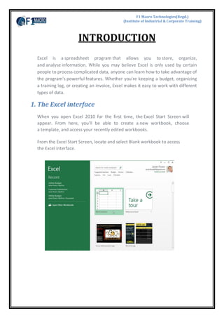
  • 1. INTRODUCTION Excel is a spreadsheet program that allows you to store, organize, and analyse information. While you may believe Excel is only used by certain people to process complicated data, anyone can learn how to take advantage of the program's powerful features. Whether you're keeping a budget, organizing a training log, or creating an invoice, Excel makes it easy to work with different types of data. 1. The Excel interface When you open Excel 2010 for the first time, the Excel Start Screen will appear. From here, you'll be able to create a new workbook, choose a template, and access your recently edited workbooks. From the Excel Start Screen, locate and select Blank workbook to access the Excel interface. F1 Macro Technologies(Regd.) (Institute of Industrial & Corporate Training)
  • 2. 2. Creating and Opening Workbooks Excel files are called workbooks. Whenever you start a new project in Excel, you'll need to create a new workbook. There are several ways to start working with a workbook in Excel 2013. You can choose to create a new workbook—either with a blank workbook or a predesigned template—or open an existing workbook. 3. To create a new blank workbook: 1. Select the File tab. backstage view will appear. 2. Select New, then click Blank workbook.
  • 3. 4. Worksheet Basics Every workbook contains at least one worksheet by default. When working with a large amount of data, you can create multiple worksheets to help organize your workbook and make it easier to find content. You can also group worksheets to quickly add information to multiple worksheets at the same time. 5. To Rename a worksheet: Whenever you create a new Excel workbook, it will contain one worksheet named Sheet1. You can rename a worksheet to better reflect its content. In our example, we will create a training log organized by month. 1. Right-click the worksheet you want to rename, then select Rename from the worksheet menu. 2. Type the desired name for the worksheet.
  • 4. 3. Click anywhere outside of the worksheet, or press Enter on your keyboard. The worksheet will be renamed. To change the default number of worksheets, navigate to Backstage view, click Options, then choose the desired number of worksheets to include in each new workbook.
  • 5. 6. To delete a worksheet: 1. Right-click the worksheet you want to delete, then select Delete from the worksheet menu. 2. The worksheet will be deleted from your workbook. 7. To copy a worksheet: If you need to duplicate the content of one worksheet to another, Excel allows you to copy an existing worksheet. 1. Right-click the worksheet you want to copy, then select Move or Copy from the worksheet menu.
  • 6. 2. The Move or Copy dialog box will appear. Choose where the sheet will appear in the Before sheet: field. In our example, we'll choose (move to end) to place the worksheet to the right of the existing worksheet. 3. Check the box next to Create a copy, then click OK 4. The worksheet will be copied. It will have the same title as the original worksheet, as well as a version number. In our example, we copied the January worksheet, so our new worksheet is named January (2). All content from the January worksheet has also been copied to the January (2) worksheet.
  • 7. You can also copy a worksheet to an entirely different workbook. You can select any workbook that is currently open from the To book: drop-down menu. 8. To move a worksheet: Sometimes you may want to move a worksheet to rearrange your workbook. 1. Select the worksheet you want to move. The cursor will become a small worksheet icon . 2. Hold and drag the mouse until a small black arrow appears above the desired location. Release the mouse. The worksheet will be moved.
  • 8. 9. To change the worksheet color: You can change a worksheet's color to help organize your worksheets and make your workbook easier to navigate. 1. Right-click the desired worksheet, and hover the mouse over Tab Color. The Color menu will appear. 2. Select the desired color. A live preview of the new worksheet color will appear as you over the mouse over different options. In our example, we'll choose Red. 10. Cell Basics Whenever you work with Excel, you'll enter information—or content— into cells. Cells are the basic building blocks of a worksheet. You'll need to learn the basics of cells and cell content to calculate, analyse, and organize data in Excel.
  • 9. 11. Understanding cells Every worksheet is made up of thousands of rectangles, which are called cells. A cell is the intersection of a row and a column. Columns are identified by letters (A, B, C), while rows are identified by numbers (1, 2, 3). Each cell has its own name—or cell address—based on its column and row. In this example, the selected cell intersects column C and row 5, so the cell address is C5. The cell address will also appear in the Name box. Note that a cell's column and row headings are highlighted when the cell is selected.
  • 10. You can also select multiple cells at the same time. A group of cells is known as a cell range. Rather than a single cell address, you will refer to a cell range using the cell addresses of the first and last cells in the cell range, separated by a colon. For example, a cell range that included cells A1, A2, A3, A4, and A5 would be written as A1:A5. In the images below, two different cell ranges are selected: Cell range A1:A8
  • 11. 12. To select a cell: To input or edit cell content, you'll first need to select the cell. 1. Click a cell to select it. 2. A border will appear around the selected cell, and the column heading and row heading will be highlighted. The cell will remain selected until you click another cell in the worksheet. 13. To select a cell range: Sometimes you may want to select a larger group of cells, or a cell range. 1. Click, hold, and drag the mouse until all of the adjoining cells you want to select are highlighted. 2. Release the mouse to select the desired cell range. The cells will remain selected until you click another cell in the worksheet.
  • 12. 14. What is Row? Rows run horizontally in an Excel worksheet. Each row is identified by a number in the row header. There are 1048576 rows in each Excel worksheet. 15. What is Column? Columns run vertically in a worksheet. Each column is identified by a letter in the column header starting with Column A and running through to Column XFD. There are 16384 columns in each excel worksheet. 16. What is Cell? The intersection point between a row and a column is called a cell. What is the hierarchy we follow in Excel? Application Workbook Worksheet Cell/Range
  • 13. 17. Around Excel sheet 18. The Quick Access toolbar Located just above the Ribbon, the Quick Access toolbar lets you access common commands no matter which tab is selected. By default, it includes the Save, Undo, and Repeat commands. You can add other commands depending on your preference. To add commands to the Quick Access toolbar: 1. Click the drop-down arrow to the right of the Quick Access toolbar. Formula Bar Active Cell Auto Filler Column Header Row Header Quick Access Toolbar RibbonTitle Bar Name Box Sheet Tabs Zoom Control Horizontal Scroll Bar Vertical Scroll Bar Column Row Cell
  • 14. 2. Select the command you want to add from the drop-down menu. To choose from more commands, select More Commands. 3. The command will be added to the Quick Access toolbar. Functions A function is a predefined formula that performs calculations using specific values in a particular order. Excel includes many common functions that can be useful for quickly finding the sum, average, count, maximum value, and minimum value for a range of cells. In order to use functions correctly, you'll need to understand the different parts of a function and how to create arguments to calculate values and cell references.
  • 15. 19. The parts of a function In order to work correctly, a function must be written a specific way, which is called the syntax. The basic syntax for a function is the equals sign (=), the function name (SUM, for example), and one or more arguments. Arguments contain the information you want to calculate. The function in the example below would add the values of the cell range A1:A20. Age Calculation: Datedif Function The DATEDIF function computes the difference between two dates in a variety of different intervals, such as the number of years, months, or days between the dates. Parameters:- 1. Date of Joining, Date of Birth or Start Date 2. End Date or Today's Date 3. Interval Syntax:- =Datedif(Start Date, End Date, "Interval")
  • 16. 20. How to Use Excel DATEDIF function:- Now, let’s understand how to use DATEDIF function in excel. Objective: Let’s, consider our objective is to find the number of days from 14 April 1912 (The day on which Titanic Sank) till todays date. So, we will try to apply the DATEDIF formula. ‘Start_Date’: In this case our ‘Start_Date’ will be: 14 April 1912. ‘End_Date’: End_Date will be today’s date. So, instead of entering the today’s date manually we will use theToday() function. ‘Unit’: As we want to find the number of days between the period. So, the ‘Unit’ will be “d”.
  • 17. This formula results into: 36910 days. Example:- 21. String & Text Functions in Excel Concatenate One of the text functions, to join two or more text strings into one string. Syntax:- =CONCATENATE (text1, [text2] ...) Example-1:-
  • 18. Example-2:- Example-3:- Note: - You can used "&" to join two words Lower The LOWER function will convert all letters in a text string to lowercase Syntax:- = Lower (Text) Example:- Upper The UPPER function will convert all letters in a text string to uppercase. Syntax:- = Upper (Text) Example:-
  • 19. Proper The PROPER function will convert a text string to proper case. That is, the first letter in each word in uppercase, and all other letters in lowercase. Syntax:- = Proper (Text) Example:- Trim The TRIM function returns a string with extra spaces, starting spaces and ending spaces removed. The CLEAN function removes nonprintable characters from a string. Syntax:- = Trim (Text) Example:- Left The Excel Left function returns a specified number of characters from the start of a supplied text string. Syntax:- = LEFT (text, [num_chars]) Text: - The original text string. [num_chars]:- An optional argument that specifies the number of characters to be returned from the start of the supplied text. If omitted, the [num_chars] argument takes on the default value of 1.
  • 20. Note: The argument given in square bracket i.e. [] is optional Example:- Right The Excel Right function returns a specified number of characters from the end of a supplied text string. Syntax:- = RIGHT (text, [num_chars]) Text: - The original text string. [num_chars]:- An optional argument that specifies the number of characters to be returned from the start of the supplied text. If omitted, the [num_chars] argument takes on the default value of 1. Note: The argument given in square bracket i.e. [] is optional Example:- Note: To learn more about Find & Len function click on below button.
  • 21. MID The Excel Mid function returns a specified number of characters from the middle of a supplied text string. Syntax:- = MID( text, start_num, num_chars ) Text: - The original text string. [start_num]:- An integer that specifies the position of the first character that you want to be returned [num_chars]:- An optional argument that specifies the number of characters to be returned from the start of the supplied text. If omitted, the [num_chars] argument takes on the default value of 1. Note: The argument given in square bracket i.e. [] is optional Example:- Note: To learn more about FIND AND LEN function click on below button. Len The Excel LEN function returns the length of a supplied text string Syntax:- = LEN( text ) Text: - Text argument is the text string that you want to find the length of. Example:-
  • 22. Find The Excel FIND function returns the position of a specified character or sub-string within a supplied text string The Find function is case-sensitive. If you want to perform a non-case-sensitive search, use the Excel Search function instead Syntax:- = FIND( find_text, within_text, [start_num] ) find_text: - The character or sub-string that you wish to find. within_text:- The text string that is to be searched [start_num]:- An optional argument that specifies the position in the within_text string, from which the search should begin If omitted, this takes on the default value of 1 (i.e. begin the search at the start of the within_text string) If the supplied find_text is found, the Find function returns a number that represents the position of the find_text in the within_text. If the supplied find_text is not found, the function returns the Excel #VALUE! error. Example:- Note: To find out the second position of the same character in a text supplied, then skip the first position of that character. Substitute The Excel Substitute function replaces occurrences of a search text string, within an original text string, with the supplied replacement text. Syntax:- = SUBSTITUTE( text, old_text, new_text, [instance_num] ) text: - The original text string containing the text to be replaced. old_text:- The text to be found and replaced by new_text. new_text :- The new text that is to be used to replace the old_text.
  • 23. instance_num :- An optional argument which specifies which occurrence of old_text should be replaced by the new_text If a value of [instance_Num] is specified, just that instance of the old_text is replaced; Otherwise, all instances of old_text are replaced with the new_text. Example:- Text The Excel TEXT function converts a supplied numeric value into text, in a user-specified format. Syntax:- = TEXT( value, format_text ) value:- A numeric value, that you want to be converted into text. format_text:- A text string that defines the formatting that you want to be applied to the supplied value new_text :- The new text that is to be used to replace the old_text. Formats Definition 0 Forces the display of a digit in its place . Defines the position that the decimal place takes D Day of the month or day of week d = one or two digit representation (eg. 1, 12) dd = 2 digit representation (eg. 01, 12) ddd = abbreviated day of week (eg. Mon, Tue) dddd = full name of day of week (eg. Monday, Tuesday) m Month (when used as part of a date) m = one or two digit representation (eg. 1, 12) mm = two digit representation (eg. 01, 12) mmm = abbreviated month name (eg. Jan, Dec) mmmm = full name of month (eg. January, December) y Year yy = 2-digit representation of year(eg. 99, 08) yyyy = 4-digit representation of year(eg. 1999, 2008) h Hour h = one or two digit representation (eg. 1, 20) h = two digit representation (eg. 01, 20) m Minute (when used as a part of a time)
  • 24. m = one or two digit representation (eg. 1, 55) m = two digit representation (eg. 01, 55) s Second s = one or two digit representation (eg. 1, 45) ss = two digit representation (eg. 01, 45) AM/PM Indicates that a time should be represented using a 12-hour clock, followed by "AM" or "PM" Example:- Trim The TRIM function returns a string with extra spaces, starting spaces and ending spaces removed. Syntax:- = Trim(text) Text:-The text value to remove the leading and trailing spaces from. Exact
  • 25. The Microsoft Excel EXACT function compares two strings and returns TRUE if both values are the same. Otherwise, it will return FALSE. Syntax:- = Trim(value1,value2 ...) Text1 and text2 The two string values to compare Example:- Search The Microsoft Excel SEARCH function returns the location of a substring in a string. The search is NOT case-sensitive. Syntax Search(substring, string, start_position) Substring The substring that you want to find. string
  • 26. The string to search within. start_position Optional. It is the position in string where the search will start. The first position is 1. Code The Microsoft Excel CODE function returns the ASCII value of a character or the first character in a cell. Syntax:- code(text) text The specified character to retrieve the ASCII value for. If there is more than one character, the function will return the ASCII value for the first character and ignore all of the characters after the first.
  • 27. Char The Microsoft Excel CHAR function returns the character based on the ASCII value. Syntax:- Char(ascii_value) ascii_value The ASCII value used to retrieve the character.
  • 28. 22. Statistical / Mathematical Functions Count To count the number of cells that contain numbers, use the COUNT function. Syntax:- = COUNT(value1, [value2], ...) Example:- Counta The COUNTA function counts the number of cells that are not empty in a range i.e. it counts everything except blank cells. Syntax:- = COUNTA (value1, [value2], ...) Countblank The COUNTBLANK function Counts empty cells in a specified range of cells. Syntax:- = COUNTBLANK(RANGE) Example:-
  • 29. Countif Count if function count the number of cells that meet a particular criteria; i.e. it counts as per the criteria and only single criteria can be used. Syntax:- = COUNTIF (range, criteria) Example:- Max The Microsoft Excel MAX function returns the largest value from the numbers provided. Syntax:- = Max(Number1…,*number2,...number_n+) number1 It can be a number, named range, array, or reference to a number. number2 ... number_n Optional. These are numeric values that can be numbers, named ranges, arrays, or references to numbers. There can be up to 30 values entered.
  • 30. Min The Microsoft Excel MIN function returns the smallest value from the numbers provided. Syntax:- = Max(Number1…,*number2,...number_n+)
  • 31. Small The Microsoft Excel SMALL function returns the nth smallest value from a set of values. Syntax:- = Small(array, nth_position) Large The Microsoft Excel LARGE function returns the nth largest value from a set of values. Syntax:- = Large(array, nth_position)
  • 32. Sum The Microsoft Excel SUM function adds all numbers in a range of cells and returns the result.. Syntax:- =sum(number1,[number2….number]) Sumif The SUMIF function is a worksheet function that adds all numbers in a range of cells based on one criteria Syntax:- =Sumif(range,criteria,[sum range])
  • 33. Sumifs The Microsoft Excel SUMIFS function adds all numbers in a range of cells, based on a single or multiple criteria Syntax:- =sumifs( sum_range, criteria_range1, criteria1, [criteria_range2, criteria2, ... criteria_range_n, criteria_n] ) Parameters or Arguments sum_range The cells to sum. criteria_range1 The range of cells that you want to apply criteria1 against. criteria1 It is used to determine which cells to add. criteria1 is applied against criteria_range1. criteria_range2, ... criteria_range_n Optional. It is the range of cells that you want to apply criteria2, ... criteria_n against. There can be up to 127 ranges. criteria2, ... criteria_n Optional. It is used to determine which cells to add. criteria2 is applied against criteria_range2, criteria3 is applied againstcriteria_range3, and so on. There can be up to 127 criteria.
  • 34. Countifs The Microsoft Excel COUNTIFS function counts the number of cells in a range, that meets a single or multiple criteria Syntax:- COUNTIFS( criteria_range1, criteria1, [criteria_range2, criteria2, ... criteria_range_n, criteria_n] ) Parameters or Arguments criteria_range1 The range of cells that you want to apply criteria1 against. criteria1 The criteria used to determine which cells to count. criteria1 is applied against criteria_range1. criteria_range2, ... criteria_range_n Optional. It is the range of cells that you want to apply criteria2, ... criteria_n against. There can be up to 127 ranges. criteria2, ... criteria_n Optional. It is used to determine which cells to count. criteria2 is applied against criteria_range2, criteria3 is applied againstcriteria_range3, and so on. There can be up to 127 criteria.
  • 35. Round The Microsoft Excel ROUND function returns a number rounded to a specified number of digits. Syntax:- =round(number,digits) Parameters or Arguments Number The number to round. Digits The number of digits to round the number to.
  • 36. Roundup The Microsoft Excel ROUNDUP function returns a number rounded up to a specified number of digits. Syntax:- =round(number,digits) Parameters or Arguments number The number to round up. digits The number of digits to round the number up to
  • 37. Rounddown The Microsoft Excel ROUNDDOWN function returns a number rounded down to a specified number of digits. Syntax:- =round (number, digits) Parameters or Arguments Number The number to round up. Digits The number of digits to round the number down to Sumproduct The Microsoft Excel SUMPRODUCT function multiplies the corresponding items in the arrays and returns the sum of the results. Syntax:- SUMPRODUCT (array1, [array2, array_n] ) Parameters or Arguments array1, array2, array
  • 38. The ranges of cells or arrays that you wish to multiply. All arrays must have the same number of rows and columns. You must enter at least 2 arrays and you can have up to 30 arrays. Mod The Microsoft Excel MOD function returns the remainder after a number is divided by a divisor. Syntax:- Mod( Number,divisor )
  • 39. Randbetween The Microsoft Excel RANDBETWEEN function returns a random number that is between a bottom and top range. The RANDBETWEEN function returns a new random number each time your spreadsheet recalculates. Syntax:- Randbetween(bottom,top) Parameters or Arguments bottom The smallest integer value that the function will return. top The largest integer value that the function will return.
  • 40. Average The Microsoft Excel AVERAGE function returns the average (arithmetic mean) of the numbers provided. Syntax:- =Avergae(number1..,number2..,number3…) 23. Information Functions Cell The Microsoft Excel CELL function can be used to retrieve information about a cell. This can include contents, formatting, size, etc. Syntax:-
  • 41. =cell(Type,[range]) Value Explanation "address" Address of the cell. If the cell refers to a range, it is the first cell in the range. "col" Column number of the cell. "color" Returns 1 if the color is a negative value; Otherwise it returns 0. "contents" Contents of the upper-left cell. "filename" Filename of the file that contains reference. "format" Number format of the cell. See example formats below. "parentheses" Returns 1 if the cell is formatted with parentheses; Otherwise, it returns 0. "prefix" Label prefix for the cell. * Returns a single quote (') if the cell is left-aligned. * Returns a double quote (") if the cell is right-aligned. * Returns a caret (^) if the cell is center-aligned. * Returns a back slash () if the cell is fill-aligned. * Returns an empty text value for all others. "protect" Returns 1 if the cell is locked. Returns 0 if the cell is not locked. "row" Row number of the cell. "type" Returns "b" if the cell is empty. Returns "l" if the cell contains a text constant. Returns "v" for all others. "width" Column width of the cell, rounded to the nearest integer.
  • 42. Isblank The Microsoft Excel ISBLANK function can be used to check for blank or null values Syntax:- =isblank(Value)
  • 43. Iserror The Microsoft Excel ISERROR function can be used to check for error values Syntax:- =isblank(Value)
  • 44. Istext The Microsoft Excel ISTEXT function can be used to check for a text value Syntax:- =isblank(Value) Isnumber The Microsoft Excel ISNUMBER function can be used to check for a Number value Syntax:- =isblank(Value)
  • 45. 24. Logical Functions If The Microsoft Excel IF function returns one value if the condition is TRUE, or another value if the condition is FALSE. Syntax:- = IF( condition, [value_if_true], [value_if_false] ) And The Microsoft Excel AND function returns TRUE if all conditions are TRUE. It returns FALSE if any of the conditions are FALSE. Syntax:- = AND( condition1, [condition2], ... ) Parameters or Arguments condition1 The first condition to test whether it is TRUE or FALSE. condition2, ...
  • 46. Optional. Additional conditions to test whether they are TRUE or FALSE. There can be up to 30 conditions in total. Or The Microsoft Excel OR function returns TRUE if any of the conditions are TRUE. Otherwise, it returns FALSE. Syntax:- = or( condition1, [condition2], ... )
  • 47. Iferror Returns a value you specify if a formula evaluates to an error; otherwise, returns the result of the formula. Use the IFERROR function to trap and handle errors in a formula. Syntax: IFERROR(value, value_if_error) 25. Database Functions Dsum The Microsoft Excel DSUM function sums the numbers in a column or database that meets a given criteria. Syntax: =DSUM( range, field, criteria ) range The range of cells that you want to apply the criteria against. field The column to sum the values. You can either specify the numerical position of the column in the list or the column label in double quotation marks. criteria The range of cells that contains your criteria.
  • 48. Dcount The Microsoft Excel DCOUNT function returns the number of cells in a column or database that contains numerc values and meets a given criteria. Syntax: =Dcount( range, field, criteria ) Parameters or Arguments range The range of cells that you want to apply the criteria against. field Optional. It is the column to count the numeric values that meet the criteria. You can either specify the numerical position of the column in the list or the column label in double quotation marks. If field is omitted, it will count all records that match the criteria. criteria The range of cells that contains your criteria.
  • 49. Daverage The Microsoft Excel DAVERAGE function averages all numbers in a column in a list or database, based on a given criteria. Syntax: =Daverage( range, field, criteria ) Parameters or Arguments range The range of cells that you want to apply the criteria against. field The column to average the values. You can either specify the numerical position of the column in the list or the column label in double quotation marks. criteria The range of cells that contains your criteria.
  • 50. Dmax The Microsoft Excel DMAX function returns the largest number in a column in a list or database, based on a given criteria. Syntax: =Dmax( range, field, criteria ) Parameters or Arguments database The range of cells that you want to apply the criteria against. field The column to find the largest number in. You can either specify the numerical position of the column in the list or the column label in double quotation marks. criteria The range of cells that contains your criteria.
  • 51. Dmin The Microsoft Excel DMIN function returns the smallest number in a column in a list or database, based on a given criteria. Syntax: =Dmin( range, field, criteria ) Parameters or Arguments database The range of cells that you want to apply the criteria against. field The column to find the smallest number in. You can either specify the numerical position of the column in the list or the column label in double quotation marks. criteria The range of cells that contains your criteria.
  • 52. Dcounta The Microsoft Excel DCOUNTA function returns the number of cells in a column or database that contains nonblank values and meets a given criteria. Syntax: =Dcounta( range, field, criteria ) Parameters or Arguments range The range of cells that you want to apply the criteria against. field The column to count the values. You can either specify the numerical position of the column in the list or the column label in double quotation marks. criteria The range of cells that contains your criteria.
  • 53. 26. Date & Time Functions Datedif The Microsoft Excel DATEDIF function returns the difference between two date values, based on the interval specified. Syntax: =Datedif(Start Date, End Date, "Interval") Parameters:- Date of Joining, Date of Birth or Start Date End Date or Today's Date Interval Interval Meaning Description M Months Complete calendar months between the dates. D Days Number of days between the dates. Y Years Complete calendar years between the dates. YM Months Excluding Years Complete calendar months between the dates as if they were of the same year. YD Days Excluding Years Complete calendar days between the dates as if they were of the same year.
  • 54. MD Days Excluding Years And Months Complete calendar days between the dates as if they were of the same month and same year. Weekday The Microsoft Excel WEEKDAY function returns a number representing the day of the week, given a date value Syntax: = WEEKDAY( serial_number, [return_value] ) Parameters:- Parameters or Arguments serial_number A date expressed as a serial number or a date in quotation marks. return_value Optional. It determines the day to use as the first day of the week in the calculations.
  • 55. Weeknum Returns the week number of a specific date. For example, the week containing January 1 is the first week of the year, and is numbered week 1. Syntax: = Weeknum( serial_number, [return_value] ) Parameters:- Serial_number Required. A date within the week. Dates should be entered by using the DATE function, or as results of other formulas or functions. For example, use DATE(2008,5,23) for the 23rd day of May, 2008. Problems can occur if dates are entered as text. Return_type Optional. A number that determines on which day the week begins. The default is 1.
  • 56. Networkdays The Microsoft Excel NETWORKDAYS function returns the number of "work days" between 2 dates, excluding weekends and holidays. Syntax: = Weeknum( start_date,end_date,[holidays] ) Parameters or Arguments start_date The start date to use in the calculation. It must be entered using the DATE function. end_date The end date to use in the calculation. It must be entered using the DATE function. holidays Optional. It is the list of holidays to exclude from the "work days" calculation. It can be entered either as a range of cells that contain the holiday dates.
  • 57. Time The Microsoft Excel TIME function returns the decimal number for a particular time. Syntax: = Weeknum( hour ,minute ,second ) Parameters or Arguments hour A number from 0 to 23, representing the hour. minute A number from 0 to 59, representing the minute. second A number from 0 to 59, representing the second.
  • 58. Hour The Microsoft Excel HOUR function returns the hour of a time value (from 0 to 23). Syntax: = hour( serial_number) Parameters or Arguments serial_number The time value to extract the hour from. It may be expressed as a string value, a decimal number, or the result of a formula.
  • 59. Minute The Microsoft Excel MINUTE function returns the minute of a time value (from 0 to 59). Syntax: =Minute( serial_number)
  • 60. Second The Microsoft Excel SECOND function returns the second of a time value (from 0 to 59) Syntax: =Second( serial_number)
  • 61. Today The Microsoft Excel TODAY function returns the current system date. This function will refresh the date whenever the worksheet recalculates. Syntax: =Today() Now The Microsoft Excel NOW function returns the current system date and time. The NOW function will refresh the date/time value whenever the worksheet recalculates. Syntax: =Now()
  • 62. Date The Microsoft Excel DATE function returns the serial number of a date. Syntax: =date (year, month, date)
  • 63. Day The Microsoft Excel DAY function returns the day of the month (a number from 1 to 31) given a date value. Syntax: =Day(date_value) Month The Microsoft Excel MONTH function returns the month (a number from 1 to 12) given a date value. Syntax: =Month(date_value)
  • 64. Year The Microsoft Excel YEAR function returns a four-digit year (a number from 1900 to 9999) given a date value. Syntax: =year(date_value) 27.Lookup Functions Vlookup The VLOOKUP function performs a vertical lookup by searching for a value in the first column of a table and returning the value in the same row in the index_number position. Syntax: =vlookup (value, table, index_number, [not_exact_match] Parameters or Arguments value The value to search for in the first column of the table. table Two or more columns of data that is sorted in ascending order. index_number
  • 65. The column number in table from which the matching value must be returned. The first column is 1. not_exact_match Optional. It determines if you are looking for an exact match based on value. Enter FALSE to find an exact match. Enter TRUE to find an approximate match, which means that if an exact match is not found, then the next smaller value is returned. If this parameter is omitted, the VLOOKUP function defaults to TRUE. Hlookup The Microsoft Excel HLOOKUP function performs a horizontal lookup by searching for a value in the top row of the table and returning the value in the same column based on the index_number. Syntax: =Hlookup (value, table, index_number, [not_exact_match]
  • 66. Index The Microsoft Excel INDEX function returns either the value or the reference to a value from a table or range. There are 2 syntaxes for the INDEX function Syntax: =INDEX( array, row_number, [column_number] ) Parameters or Arguments array A range of cells or table. row_number The row number in the array to use to return the value. column_number Optional. It is the column number in the array to use to return the value.
  • 67. Match The Microsoft Excel MATCH function searches for a value in an array and returns the relative position of that item. Syntax: =MATCH( value, array, [match_type] ) Parameters or Arguments value The value to search for in the array. array A range of cells that contains the value that you are searching for. match_type Optional. It the type of match that the function will perform. The possible values are:
  • 68. Row The Microsoft Excel ROW function returns the row number of a cell reference. Syntax: =Row( reference )
  • 69. Column The Microsoft Excel COLUMN function returns the column number of a cell reference. Syntax: =Column ( reference ) Transpose The Microsoft Excel TRANSPOSE function returns a transposed range of cells. For example, a horizontal range of cells is returned if a vertical range is entered as a parameter. Or a vertical range of cells is returned if a horizontal range of cells is entered as a parameter. =Transpose (range)
  • 70. Offset The Microsoft Excel OFFSET function returns a reference to a range that is offset a number of rows and columns from another range or cell. Syntax: =OFFSET( range, rows, columns, [height], [width] ) Parameters or Arguments Range The starting range from which the offset will be applied. Rows The number of rows to apply as the offset to the range. This can be a positive or negative number. Columns The number of columns to apply as the offset to the range. This can be a positive or negative number. Height Optional. It is the number of rows that you want the returned range to be. If this parameter is omitted, it is assumed to be the height ofrange.
  • 71. Width It is the number of columns that you want the returned range to be. If this parameter is omitted, it is assumed to be the width of range. Choose The Microsoft Excel CHOOSE function returns a value from a list of values based on a given position. Syntax: =CHOOSE( position, value1, [value2, ... value_n] ) Parameters or Arguments position The position number in the list of values to return. It must be a number between 1 and 29. value1, value2, ... value_n A list of up to 29 values. A value can be any one of the following: a number, a cell reference, a defined name, a formula/function, or a text value.
  • 72. 28. Advance Validation Data validation in Excel to make sure that users enter certain values into a cell that you allow him to enter. In this example, we restrict users to enter a whole number between 0 and 10. 1. Select cell A2. 2. On the Data tab, click Data Validation. 3. In the Allow list, click Whole number. 4. In the Data list, click between. 5. Enter the Minimum and Maximum values.
  • 73. Input Message : Input messages appear when the user selects the cell and tell the user what to enter. 1. Check 'Show input message when cell is selected'. 2. Enter a title. 3. Enter an input message. Error Alert If users ignore the input message and enter a number that is not valid, you can show them an error alert. 1. Check 'Show error alert after invalid data is entered'. 2. Enter a title. Data Validation Result 1. Select cell C2. 2. Try to enter a number higher than 10.
  • 74. 29. Conditional Formatting Enhancements to conditional formatting are a popular feature in Microsoft Excel. Analysing data has never been more interesting and colourful. Now, you can track trends, check status, spot data, and find top values like never before. We will start off with creating simple worksheet of students, which includes; Name of the student, and obtained Marks in their respective courses. Select Full Data Goto Home Tab conditional formatting .
  • 75. Apply conditional formatting styles then ok. 2. Highlight Order Amount highest to lowest with Data
  • 76. 30. Sheet Protection When you share a file with other users, you may want to protect a worksheet to help prevent it from being changed. 1. Right click a worksheet tab. 2. Click Protect Sheet. 3. Enter a password. 4. Check the actions you allow the users of your worksheet to perform. 5. Click OK. Note: if you don't check any action, users can only view the Excel file!
  • 77. 31. Workbook Protection 1. Save as the existing file you want to protect. 2. Click on Tool Option and Select General Option. 3. Click on General Options. 4. Enter Password to open and Password to modify. 5. Confirm both the password to match and then save as with the name you want to enter.
  • 78. 32. Share Workbook If you share a workbook, you can work with other people on the same workbook at the same time. The workbook should be saved to a network location where other people can open it. You can keep track of the changes other people make and accept or reject those changes. 1. On the Review tab, in the Changes group, click Share Workbook. 2. On the Editing tab, click the check box and click OK.
  • 79.
  • 80. 33. Pivot Tables Pivot tables are one of Excel's most powerful features. A pivot table allows you to extract the significance from a large, detailed data set. Our data set consists of 214 rows and 6 fields. Order ID, Product, Category, Amount, Date and Country. 'To insert a pivot table, execute the following steps. 1. Click any single cell inside the data set. 2. On the Insert tab, click PivotTable. The following dialog box appears. Excel automatically selects the data for you. The default location for a new pivot table is New Worksheet. 3. Click OK.
  • 81. Drag fields The PivotTable field list appears. To get the total amount exported of each product, drag the following fields to the different areas. 1. Product Field to the Row Labels area. 2. Amount Field to the Values area. 3. Country Field to the Report Filter area.
  • 82. 'Below you can find the pivot table. Bananas are our main export product. That's how easy pivot tables can be!
  • 83. 34.Using advanced filters Advanced text filters can be used to display more specific information, such as cells that contain a certain number of characters or data that does not contain a word you specify. In this example, we'll use advanced text filters to hide any equipment that is related to cameras, including digital cameras and camcorders. 1. From the Data tab, click the Filter command. 2. Click the drop-down arrow in the column of text you want to filter. In this example, we'll filter the Equipment Detail column to view only certain types of equipment. 3. Choose Text Filters to open the advanced filtering menu. 4. Choose a filter. In this example, we will choose Does Not Contain to view data that does not contain the text we specify. 5. The Custom AutoFilter dialog box appears. 6. Enter your text to the right of your filter. In this example, we'll enter cam to View data that does not contain these letters. That will exclude any equipment Related to cameras, such as digital cameras, camcorders, camera bags, and the digital printer.
  • 84. 7. Ok 35. Sorting This Excel tutorial explains how to sort data in alphabetical order based on one column in Excel 2010 (with screenshots and step-by-step instructions). In Microsoft Excel 2010, I'm trying to put a chart in alphabetical order. There are 4 columns and over 2,000+ rows of information. I need to sort the data by column B (ie: Product column) in alphabetical order. How do I do this? To apply a sort in Excel, highlight the data that you wish to sort. Then select the Data tab from the toolbar at the top of the screen and click on the Sort button in the Sort & Filter group. Wh en the Sor t win do w ap pe ars,
  • 85. select the data that you wish to sort by. In this example, we want to sort by the Product column (column B) in alphabetical order (A to Z). Click on the OK button. Now when you return to the spreadsheet, the data should be sorted. 36.Remove Duplicates 1. Select the data from where you want to remove the duplicates. 2. On the Data tab, click Remove Duplicates. 3. Leave all check boxes checked and click OK.
  • 86. 4. Then Ok. 37. Calculation Type Automatic Calculation Automatic calculation mode means that Excel will automatically recalculate all open workbooks at each and every change, and whenever you open a workbook. Manual Calculation Manual calculation mode means that Excel will only recalculate all open workbooks when you request it by pressing F9 or Ctrl-Alt-F9, or when you Save a workbook. For workbooks taking more than a fraction of a second to recalculate it is usually better to set Calculation to Manual
  • 87. 38. Type of Reference in Excel Relative Reference By default, Excel uses relative reference, In cell D9 to D11 the cell reference B9,B10,B11,C9,C10,C11 are realtive reference(i.e. Unfreeze cells) Absolute Reference To create an absolute reference, place a $ symbol in front of the column letter and row number of cell(i.e. we need to freeze H19 cell to add the bonus to each employee)
  • 88. Mixed Reference Sometimes we need a combination of relative and absolute reference (mixed reference). 39. Goal Seek Let's say you're enrolled in a class. You currently have a grade of 65, and you need at least a 70 to pass the class. Luckily, you have one final assignment that might be able to raise your average. You can use Goal Seek to find outwhat grade you need on the final assignment to pass the class. In the image below, you can see that the grades on the first four assignments are 58, 70, 72, and 60. Even though we don't know what the fifth grade will be, we can write a formula—or function—that calculates the final grade. In this case, each assignment is weighted equally, so all we have to do is average all five grades by typing=AVERAGE(B2:B6). Once we use Goal Seek, cell B6 will show us the minimum grade we'll need to make on that assignment. 1. Select the cell whose value you want to change. Whenever you use Goal Seek, you'll need to select a cell that already contains
  • 89. a formula or function. In our example, we'll select cell B7 because it contains the formula=AVERAGE(B2:B6). 2. From the Data tab, click the What-If Analysis command, then select Goal Seek from the drop-down menu. 3. A dialog box will appear with three fields: o Set cell: This is the cell that will contain the desired result. In our example, cell B7 is already selected. o To value: This is the desired result. In our example, we'll enter 70 because we need to earn at least that to pass the class. o By changing cell: This is the cell where Goal Seek will place its answer. In our example, we'll select cell B6because we want to determine the grade we need to earn on the final assignment. 4. When you're done, click OK.
  • 90. 5. The dialog box will tell you if Goal Seek was able to find a solution. Click OK. 6. The result will appear in the specified cell. In our example, Goal Seek calculated that we will need to score at least a 90 on the final assignment to earn a passing grade.
  • 91. 40. Scenario Manager Assume you own a book store and have 100 books in storage. You sell a certain % for the highest price of $50 and a certain % for the lower price of $20. If you sell 60% for the highest price, cell D10 calculates a total profit of 60 * $50 + 40 * $20 = $3800. Create Different Scenarios But what if you sell 70% for the highest price? And what if you sell 80% for the highest price? Or 90%, or even 100%? Each different percentage is a different scenario. You can use the Scenario Manager to create these scenarios. Note: You can simply type in a different percentage into cell C4 to see the corresponding result of a scenario in cell D10. However, what-if analysis enables you to easily compare the results of different scenarios. Read on. 1. On the Data tab, click What-If Analysis and select Scenario Manager from the list.
  • 92. The Scenario Manager dialog box appears. 2. Add a scenario by clicking on Add. 3. Type a name (60% highest), select cell C4 (% sold for the highest price) for the Changing cells and click on OK.
  • 93. 4. Enter the corresponding value 0.6 and click on OK again. 5. Next, add 4 other scenarios (70%, 80%, 90% and 100%). Finally, your Scenario Manager should be consistent with the picture below:
  • 94. Scenario Summary To easily compare the results of these scenarios, execute the following steps. 1. Click the Summary button in the Scenario Manager. 2. Next, select cell D10 (total profit) for the result cell and click on OK. Result: Conclusion: if you sell 70% for the highest price, you obtain a total profit of $4100, if you sell 80% for the highest price, you obtain a total profit of $4400, etc. That's how easy what-if analysis in Excel can be. 41. Data Table To create a two-variable data table in Excel 2013, you enter two ranges of possible input values for the same formula in the Data Table dialog box: a range of values for the Row Input Cell across the first row of the table and a range of values for the Column Input Cell down the first column of the table. You then enter the formula (or a copy of it) in the cell located at the intersection of this row and column of input values
  • 95. =Sales_2013+(Sales_2013*Growth_2014) - (Sales_2013* Expenses_2014 To set up the two-variable data table, add a row of possible Expenses_2014 percentages in the range C7:F7 to a column of possible Growth_2014 percentages in the range B8:B17.Then, copy the original formula named Projected_Sales_2014 from cell B5 to cell B7, the cell at the intersection of this row of Expenses_2014 percentages and column of Growth_2014 percentages with the formula: =Projected_Sales_2014 With these few steps, you can create a two-variable data table : 1. Select the cell range B7:F17. This cell range incorporates the copy of the original formula along with the row of possible expenses and growth-rate percentages.
  • 96. 2. Click Data→What-If Analysis→Data Table on the Ribbon. Excel opens the Data Table dialog box with the insertion point in the Row Input Cell text box. 3. Click cell B4 to enter the absolute cell address, $B$4, in the Row Input Cell text box. 4. Click the Column Input Cell text box and then click cell B3 to enter the absolute cell address, $B$3, in this text box. 5. Click OK to close the Data Table dialog box. 42. Paste Special Command The Paste Special dialog box offers many more paste options. To launch the Paste Special dialog box, execute the following steps. 1. Select cell B5, right click, and then click Copy (or press CTRL + c). 2. Next, select cell D5, right click, and then click Paste Special.
  • 97. The Paste Special dialog box appears.
  • 98. 43. Freeze Pane To keep an area of a worksheet visible while you scroll to another area of the worksheet, you can lock specific rows or columns in one area by freezing or splitting panes. 1. On the View tab, click Freeze Panes, Freeze Top Row. 2. On the View tab, click Freeze Panes, Freeze First Column. 3. To unlock all rows and columns, execute the following steps.
  • 99. 4. How to freeze row and column both at a same time A). Select Cell B2 and Unfreeze Pane First by following 3rd Step. B). Select the cell from where you want to freeze row and column and follow the below step as shown in below screen shot
  • 100. 44. Text to Column To separate the contents of one Excel cell into separate columns, you can use the 'Convert Text to Columns Wizard'. For example, when you want to separate a list of full names into last and first names. 1. Select the range with full names. 2. On the Data tab, click Text to Columns. 3. Choose Delimited and click Next. 4. Clear all the check boxes under Delimiters except for the Comma and Space check box.
  • 101. 5. Click Finish. Note: This example has commas and spaces as delimiters. You may have other delimiters in your data. Experiment by checking and unchecking the different check boxes. You get a live preview of how your data will be separated.