PhD Qualifying
•Als ODP, PDF herunterladen•
2 gefällt mir•927 views

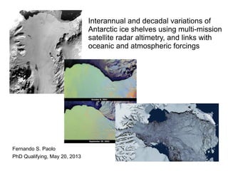
Interannual and decadal variations of Antarctic ice shelves using multi-mission satellite radar altimetry, and links with oceanic and atmospheric forcings

Empfohlen
Empfohlen
Weitere ähnliche Inhalte
Was ist angesagt?
Was ist angesagt? (20)
Ähnlich wie PhD Qualifying
Ähnlich wie PhD Qualifying (20)
PhD Qualifying
- 1. Interannual and decadal variations of Antarctic ice shelves using multi-mission satellite radar altimetry, and links with oceanic and atmospheric forcings Fernando S. Paolo PhD Qualifying, May 20, 2013 Scripps Institution of Oceanography University of California, San Diego
- 2. Presentation outline 1. Background Importance, Hypothesis, Evidence 2. Thesis Chapter 1, Chapter 2, Chapter 3 3. Summary Results and Big Picture
- 3. Why do we care? Ice-sheet mass loss Sea-level rise
- 4. Why do we care? Ice-sheet mass loss Sea-level rise Shepherd et al., 2012 Antarctica Greenland Glaciers Ice volume 3 mm/yr (~1.8 from Cryosphere)
- 5. Why Antarctica? The marine Ice-sheet instability Bed above sea level Vaughan and Arthern, 2007 Increased discharged with grounding-line retreat → unstable condition! Fig. M. Helper Data BEDMAP
- 6. Why ice shelves? ice shelves are the “interface” between the ice sheet and the ocean Fig. Ice-shelf coverage by satellite altimetry missions
- 7. Ice-shelf buttressing Compressive stress is a result of ice-shelf buttressing Hughes, 2011 OCEAN GROUNDED ICE Ice rise Confining embayment Ice rumple Calving front
- 8. Ice-shelf-ocean interaction 100s km 1-2 km Fig. M. Craven, AAD Three modes of basalt melt (Jacobs et al., 1992)
- 9. Ice-shelf-ocean heat exchange Jenkins et al., 2010 Melt rates of 10s m/yr
- 10. Ice-shelf-ocean heat exchange CDW all the way to the sub-ice-shelf cavity Melt rates of 10s m/yr Jenkins et al., 2010 Jacobs et al., 2011
- 11. Ice-shelf and grounded-ice thinning Pritchard et al., 2012
- 12. Evidence on ice-shelf buttressing Rignot et al., 2004
- 13. Previous studies ERS-1/2 1992-01 ERS-2/Envisat 1994-08 ICESat 2003-08 Zwally et al., 2005 Shepherd et al., 2010 Pritchard et al., 2012 9 years 50 km Duration Spt. Res. 14 years One trend per ice shelf 5 years 30 km To detect climate signals we need long and continuous records!
- 14. My contribution 1. Derive reliable time series of elevation change over the longest possible time period 2. Quantify long-term trends 3. Quantify interannual-to-decadal variability 4. Identify causes of temporal and spatial variability
- 15. Thesis structure Chapter 1 → The methodology (Generate the dataset) Chapter 2 → Radar-Laser comparison (Validate the dataset) Chapter 3 → Ice-shelf variability (Analyze the dataset)
- 16. Chapter 1 Constructing time series of elevation change
- 17. Satellite altimetry missions Twenty years of continuous data over the ice shelves
- 18. The challenge of multi-mission integration Differences between missions: – RA systems, orbit configurations, time spans... Radar interaction with variable surf. properties: ρs ( x , t ) ke( x , t) – Surface density, – Penetration depth, Spatial and temporal dependent corrections: – Ocean tide + load (for high lat) – Atm pressure (IBE) – Regional sea-level rise
- 19. The challenge over ice shelves Due to hydrostatic equilibrium the altimeter only see 10-15% of the grounded ice signal (in elevation change) So to increase signal-to-noise ratio requires lots of averaging both in time and space
- 20. Averaging in time Monthly averages Seasonal averages Time steps → 3-month blocks of data
- 21. Averaging in space 3 x One month of data ~750 bins with 15 to 200 observations (for FRIS)
- 22. Averaging time series 82 time series per bin (x 2) 61,500 time series for FRIS (x 2) Matrix before Matrix after
- 23. Inter-mission cross-calibration ERS-1 ERS-2 Envisat What happens when there are no data in the overlapping period?
- 24. The backscatter problem k e ( x , t ) ρs( x , t ) Remy et al., 2012 Penetration: Densification:
- 25. Backscatter correction hc (t)=h(t)−s g (t)−h0 Amplitude series Differenced series Elevation Backscatter Done for each grid-cell
- 26. Time-varying backscatter hc (t)=h(t )−s(t ) g (t )−h0(t ) ERS-1 ERS-2 Envisat Done for each grid-cell
- 27. Different corrections, different results? Amplitude ts Differenced ts
- 28. Different corrections, different results? Different fluctuation and trend Constant correlation Variable correlation Amplitude ts Differenced ts How significant are these differences?
- 29. Chapter 2 Envisat (radar) vs ICESat (laser) inter-comparison
- 30. Two altimeters, one purpose Envisat (Radar) – microwave (λ ~ 2.5 cm) – wide footprint (3 km) – all weather – continuous sampling – penetrates into snow ICESat (Laser) – visible (λ ~ 650 nm) – narrow footprint (70 m) – cloud interaction – campaign mode – top-of-snow reflection
- 31. Do they measure the same thing? First time this comparison is done in this way
- 32. Do they measure the same thing? Envisat ICESat We need an explanation for such differences! First time this comparison is done in this way
- 33. Two ways of estimating elevation changes ∂ h ∂ t Dh 1) Eulerian (fixed): 2) Lagrangian (moving): Dt =∂ h ∂ t + u⋅∇ h (t1) A (t2) A' B A'-A = Euler B-A = Lagrange
- 34. Footprint differences ICESat footprint (70 m) is about 0.05% of RA-2 footprint (3 km)
- 35. Is radar ∂ h / ∂ t Eulerian?
- 36. Is radar ∂ h / ∂ t Eulerian?
- 37. What is signal and what is noise? ICESat data are very noisy! How much can we trust? Cross-over analysis Along-track analysis Pritchard et al., 2012 Two different techniques, same pattern → features are in the data!
- 38. Chapter 3 Variability of Antarctic ice-shelf elevations
- 39. Our main goal – Search for mechanisms that could explain the observed variability in h( x , t )
- 40. Ice-shelf mass balance ∂ h ∂ t = ∂Δ ∂ t −M ∂ ∂ t ρw − M dm ∂ 1+∫0 1(m) ∂ t ρf − + (ρi −1−ρw − 1)(M˙ s+ M˙ b+ u⋅∇ M+ M ∇⋅u) Altimeter observation Sea-level variations Ocean-density changes Firn compaction Ice-ocean density contrast Surface accumulation rate Basal accumulation rate Advection of thickness gradient and flow divergence Shepherd et al., 2003; Padman et al., 2012
- 41. Variability within an ice shelf We are able to resolve the “fine” spatial scales
- 42. Spatio-temporal change in ∂ h / ∂ t Why aren't thinning/thickening regions “fixed”?
- 43. Correlations, correlations... Fig. J. Allen, NASA Data NSIDC What is the relation to sea-ice variability? – Sea ice protects ice shelves by cooling air temperatures and dampening waves. – Also affects mode 1 of basal melt. Is there any relation to climate Indices (ENSO, SAM, ZW3)? – EOF analysis on h(x,t)
- 44. Large-scale coherent events? AMERY FRIS ROSS Decadal oscillation In phase?
- 45. Thesis summary Generate a 20-year long and high resolution dataset of thickness variation for all Antarctic ice shelves. Better understand the radar altimeter signal interaction with ice surfaces, and its effect in the final estimates. Estimate long-term trends and explain the variability in Antarctic ice-shelf thickness for the last two decades.
Hinweis der Redaktion
- an ice stream entering a confined and pinned ice shelf. Shelf flow is from the ice-stream ungrounding line (heavy dashed line) to the ice-shelf calving front (hatchured line), with flow shearing along the sides of a confining embayment (half arrows alongside thick solid lines), around ice rises (half arrows alongside thin solid lines), and over ice rumples (full arrows across thin dashed lines)
- Along an ice-sheet periphery, the ocean surface waters tend to be relatively fresh and cold (Fig. 2, C and D), typically at or near the surface freezing point. The properties of such waters typically are of polar origin and have only modest impact on melting beneath ice shelves. Below these surface waters, at depths typically ranging from 100 to 1000 m, there often resides a relatively warm and salty layer of water originating from the subtropical or subpolar regions (Fig. 2, C and D). These warm waters have a large impact where they contact glacial ice, causing melting rates of orders of tens or more meters per year (right) Vertical temperature and salinity sections (a) from the CTDs shown in the Fig. 1 inset and extended beneath the PIG and (b) along the PIG calving front, looking toward the ice shelf. Both panels show temperature in colour relative to the in situ freezing point, salinity by black contours and the surface-referenced 27.75 isopycnal and potential temperature maximum by thick and thin white lines. Open circles in b show ice draft above the ridge crest (black dots) beneath the PIG, from airborne radar and Autosub measurements11
- Along an ice-sheet periphery, the ocean surface waters tend to be relatively fresh and cold (Fig. 2, C and D), typically at or near the surface freezing point. The properties of such waters typically are of polar origin and have only modest impact on melting beneath ice shelves. Below these surface waters, at depths typically ranging from 100 to 1000 m, there often resides a relatively warm and salty layer of water originating from the subtropical or subpolar regions (Fig. 2, C and D). These warm waters have a large impact where they contact glacial ice, causing melting rates of orders of tens or more meters per year (right) Vertical temperature and salinity sections (a) from the CTDs shown in the Fig. 1 inset and extended beneath the PIG and (b) along the PIG calving front, looking toward the ice shelf. Both panels show temperature in colour relative to the in situ freezing point, salinity by black contours and the surface-referenced 27.75 isopycnal and potential temperature maximum by thick and thin white lines. Open circles in b show ice draft above the ridge crest (black dots) beneath the PIG, from airborne radar and Autosub measurements11
- Arrows highlight areas of slow-flowing, grounded ice
- Accelerated ice discharge from the Antarctic Peninsula following the collapse of Larsen B ice shelf Ice velocity, V, in Jan. 1996 (black square), Oct. 2000 (red square), Dec. 2002 (blue triangle), Oct. 2003 (green triangle), Dec. 2003 (yellow triangle) vs distance, D, from the grounding line along profiles in Figure 2. Surface elevation (meters) from CECS/NASA in (b –c) and InSAR in (a) are thick black lines. Bed elevation (meters) from CECS/NASA are thick black lines in (b). In (a –c), bed elevation deduced from ice shelf elevation assuming ice to be in hydrostatic equilibrium are dotted black lines
- Three inter-related steps independently publishable
- Say something about IMBIE comparisons!!!!!!!!!!!!!!!!!!!!!
- Peterman Glacier: 80% of the thickness is removed by basal (5% by surf.) melting when it reached the ice front.
- Peterman Glacier: 80% of the thickness is removed by basal (5% by surf.) melting when it reached the ice front.
- Explain how. Frontal and full-ice-shelf time series.
- Mention coincident decadal oscilation