its for business statistics students.

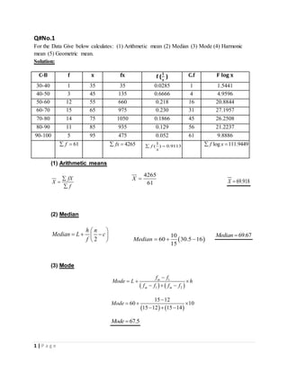
1. 1 | P a g e
Q#No.1
For the Data Give below calculates: (1) Arithmetic mean (2) Median (3) Mode (4) Harmonic
mean (5) Geometric mean.
Solution:
(1) Arithmetic means
fX
X
f



4265
61
X 
69.918X 
(2) Median
2
h n
Median L c
f
 
   
   
10
60 30.5 16
15
Median   
69.67Median 
(3) Mode
   
1
1 2
m
m m
f f
Mode L h
f f f f

  
  
   
15 12
60 10
15 12 15 14
Mode

  
  
67.5Mode 
C-B f x fx f (
𝟏
𝒙
) C.f F log x
30-40 1 35 35 0.0285 1 1.5441
40-50 3 45 135 0.6666 4 4.9596
50-60 12 55 660 0.218 16 20.8844
60-70 15 65 975 0.230 31 27.1957
70-80 14 75 1050 0.1866 45 26.2508
80-90 11 85 935 0.129 56 21.2237
90-100 5 95 475 0.052 61 9.8886
61f  4265fx  1
( ) 0.9113f
x
  log 111.9449f x 

2. 2 | P a g e
(4)Harmonic mean:
.
1
.
f
H M
f
x


 
 
 
61
.
0.9113
H M  . 66.93H M 
(5) Geometric mean:
(f logX)
. logG M anti
f



41.9449
. log
61
G M anti . 68.4227G M 
Q#NO.2
Find the (1) Arithmetic mean (2) Median (3) Mode (4) Harmonic mean (5) Geometric mean.
Solution:
(1) Arithmetic mean:
FX
X
F



18765
164
X  162.44X 
C-B f x fx Flogx f (
𝟏
𝒙
) C.f
0-40 6 20 120 7.8062 0.3 6
40-80 15 60 900 26.6723 0.25 21
80-120 22 100 2200 44 0.22 43
120-160 30 140 4200 64.3839 0.2143 73
160-200 45 180 8100 101.4873 0.25 118
200-140 27 220 5940 63.2455 0.1228 145
240-180 13 260 3380 31.3947 0.05 15.8
280-320 6 300 1800 14.8628 0.02 164
164f  26640fx  log 353.8527f x  1
( ) 1.427f
x
 

3. 3 | P a g e
(2) Median
2
h n
Median L c
f
 
   
 
 
40
160 82 73
45
Median    168Median 
(3) Mode
   
1
1 2
m
m m
f f
Mode L h
f f f f

  
  
   
45 30
160 40
45 30 45 27
Mode

  
  
   
45 30
160 40
45 30 45 27
Mode

  
  
15
160 40
33
Mode   
178.18Mode 
(4)Harmonic mean:
.
1
.
f
H M
f
x


 
 
 
164
.
1.4271
H M 
. 114.92H M 
(5) Geometric mean:
(f logX)
. logG M anti
f



353.8527
. log
164
G M anti
 . log 2.1577G M anti . 143.789G M 

4. 4 | P a g e
Q#No.3
Calculate the: (1) Arithmetic mean (2) Median (3) Mode (4) Harmonic mean (5) Geometric
mean.
Solution:
(1) Arithmetic mean:
fX
X
f



3372.5
55
X  61.318X 
(2) Median
2
h n
Median L c
f
 
   
 
 
55
60 27.5 2
18
Median    61.18Median 
(3) Mode
   
1
1 2
m
m m
f f
Mode L h
f f f f

  
  
   
18 12
60 5
18 12 18 13
Mode

  
  
30Mode 
(4)Harmonic mean:
.
1
.
f
H M
f
x


 
 
 
55
.
0.90587
H M  . 60.715H M 
C-B f X fx Flogx f (
𝟏
𝒙
) C.f
45-50 2 47.5 94 3.3533 0.0421 2
50-55 7 52.5 367.5 12.0411 0.1333 9
55-60 12 57.5 690 21.1160 0.2086 21
60-65 18 62.5 1125 32.3258 0.288 39
65-70 13 67.5 877.5 23.7809 0.1925 52
70-75 3 72.5 217.5 5.5810 0.04137 54
55f  3372.5fx  log 98.1981f x  1
( ) 0.90587f
x
 

5. 5 | P a g e
(5) Geometric mean:
(f logX)
. logG M anti
f



98.1981
. log
55
G M anti
 . log 1.78542G M anti . 61.012G M 
Q#No.4
For the Data Give below calculates: (1) Arithmetic mean (2) Median (3) Mode (4) Harmonic
mean (5) Geometric mean.
Solution:
(1) Arithmetic mean:
fX
X
f



46350
850
X  54.526X 
(2) Median
2
h n
Median L c
f
 
   
 
 
10
60 425 420
190
Median    60.263Median 
(3) Mode
   
1
1 2
m
m m
f f
Mode L h
f f f f

  
      
190 125
60 10
190 125 190 240
Mode

  
  
 
65
60 10
65 50
Mode   
 
8.333Mode 
C-B f x fx Flogx f (
𝟏
𝒙
) C.f
0-10 25 5 125 17.47 5 25
10-20 40 15 600 47.043 2.667 65
20-30 60 25 1500 83.876 2.4 125
30-40 75 35 2625 115.80 2.142 200
40-50 95 45 4275 157.05 2.111 295
50-60 125 55 6875 217.54 2.272 420
60-70 190 65 12350 344.45 2.923 610
70-80 240 75 18000 445.75 3.2 850
850f  46350fx  log 1428.98f x  1
( ) 22.75f
x
 

6. 6 | P a g e
(4) Harmonic mean:
.
1
.
f
H M
f
x


 
 
 
850
.
22.75
H M  . 37.36H M 
(5) Geometric mean:
(f logX)
. logG M anti
f



1428.98
. log
850
G M anti . 47.98G M 
Q#No.5
For the Data Give below calculates: (1) Arithmetic mean (2) Median (3) Mode (4) Harmonic
mean (5) Geometric mean.
Solution:
(1) Arithmetic mean:
fX
X
f



2005
72
X  27.847X 
(2) Median
2
h n
Median L c
f
 
   
 
 
5
22.5 36 24
19
Median    25.66Median 
C-B f X fx C.f F log x 1
f
x
 
 
 
12.5-17.5 2 15 30 2 2.3522 0.4
17.5-22.5 22 20 440 24 28.6227 1.1
22.5-27.5 19 25 475 43 26.5609 0.76
27.5-32.5 14 30 420 57 20.6797 0.4667
32.5-37.5 3 35 105 60 4.6322 0.857
37.5-42.5 4 40 160 64 6.4082 0.1
42.5-47.5 6 45 270 70 9.9193 0.1333
47.5-52.5 1 50 50 71 1.6989 0.02
52.5-57.5 1 55 55 72 1.7407 0.0181
∑f=72 ∑fx=2005 ∑flogx=102.6145 1
f
x
 
  
 

7. 7 | P a g e
(3) Mode:
   
1
1 2
m
m m
f f
Mode L h
f f f f

  
      
22 2
17.5 5
22 2 22 19
Mode

  
  
20
17.5 5
20 3
Mode   

21.85Mode 
(4) Harmonic mean:
.
1
.
f
H M
f
x


 
 
 
72
.
3.0837
H M  . 23.35H M 
(5) Geometric mean:
(f logX)
. logG M anti
f



102.6145
. log
72
G M anti . 26.62G M 

8. 8 | P a g e
Q#No.1
Calculate the correlation co-efficient between percentage of marks scored by 12 students in
statistics and economics.
Solution:
(1). Find the co-efficient of correlation:
2 2 2 2
( ) ( )
n xy x y
r
n x x n y y
   

           
2 2
12(23136) (750)(365)
12(47470) (750) 12(11385) (365)
r


       
  
3882
7140 3395
r 
710
45054900
r 
3882
4923.443917
r  0.7884r 
(2). Regression line:
Find the regression line of following data:
Y on X:
Y=a+bx
2 2
( )
yx
n xy x y
b
n x x
   

  
    
  2
12 23136 750 365
12 47470 (750)
yxb



277632 273750
569640 562500
yxb



3882
7140
yxb  0.543yxb 
X y xy 𝒙 𝟐
𝒚 𝟐
50 22 1100 2500 484
54 25 1350 2916 625
56 34 1904 3136 1156
59 25 1652 3481 784
60 26 1560 3600 678
61 30 1830 3721 900
62 32 1984 3844 1024
65 30 1950 4225 900
67 28 1876 4489 784
71 34 2414 5041 1156
71 36 2556 5041 1296
74 40 2960 5476 1600
∑x=750 ∑y=365 ∑xy=23136 ∑𝒙 𝟐=47470 ∑𝒚 𝟐=11385

9. 9 | P a g e
yx
yx
y b x
a
n
  

    365 0.543 750
12
yxa

 3.52yxa  
The estimated regression line is as follows.
ˆ 3.52 0.543Y X  
(3). Regression line:
X on Y:
X=a+by
2 2
( )
xy
n xy x y
b
n y y
   

  
    
  2
12 23136 750 365
12 11385 (365)
xyb



277632 27375
136620 133225
xyb



3882
3395
xyb  1.143xyb 
.
xy
x bxy y
a
n
  

   750 1.143 (365)
12
xya

 27.73xya 
The estimated regression line is as follows.
ˆ 27.73 1.143x Y 

10. 10 | P a g e
Q#No.2
Calculate the Co-efficientof correlationfromthe followingdataandalsocompute RegressionlineY onX
Solution:
(1).Find the co-efficient of correlation:
2 2 2 2
( ) ( )
n xy x y
r
n x x n y y
   

           
2 2
(11)(1336) (110)(125)
(11)(1210) (110) (11)(153) (125)
r


       
14696 13750
(13310 12100)(16841 15625)
r


 
946
(1210)(1216)
r 
946
1471360
r 
946
1212.99
r  0.779r 
(2). Regression line:
Y on X
Y a bx 
2 2
( )
yx
n xy x y
b
n x x
   

   2
(11)(1336) (110)(125)
(11)(1210) (110)
yxb



(14696) (13750)
(13310) (12100)
yxb



946
1210
yxb  0.781yxb 
X Y XY 𝒙 𝟐
𝒚 𝟐
5 9 45 25 81
6 6 36 36 36
7 10 70 49 100
8 8 64 64 64
9 13 117 81 169
10 11 110 100 121
11 14 154 121 196
12 10 120 144 100
13 14 182 169 196
14 12 168 196 144
15 18 270 225 324
∑X=110 ∑Y=125 ∑XY=1336 ∑𝑿 𝟐
=1240 ∑𝒀 𝟐
=1531

11. 11 | P a g e
yx
yx
y b x
a
n
  

(125) (0.781)(110)
11
yxa


125 85.91
11
yxa


39.09
11
yxa  3.553yxa 
The estimated regression line is as follows.
ˆ 3.553 0.781Y x 
Q#NO.3
Calculate the Co-efficient of correlation from the following data and also compute Regression
line Y on X and X on Y.
Solution:
(1). Find the co-efficient of correlation:
2 2 2 2
( ) ( )
n xy x y
r
n x x n y y
   

           
2 2
(10)(33535) (655)(500)
(10)(46059) (655) (10)(25464) (500)
r


       
(335350) (327500)
(460590 429025)(254640 250000)
r


 
(7850)
(31565)(4640)
r 
X Y XY 𝒙 𝟐
𝒚 𝟐
16 40 640 256 1600
72 52 3744 5184 2704
73 43 3139 5329 1849
63 49 3087 3969 2401
83 61 5063 6889 3721
80 58 4640 6400 3364
66 44 2904 4359 1936
66 58 3828 4356 3364
74 50 3700 5476 2500
62 45 2790 3844 2025
∑X=655 ∑Y=500 ∑XY=33535 ∑𝑿 𝟐
=46059 ∑𝒀 𝟐
=25464

12. 12 | P a g e
(7850)
12102.13204
r  0.6486r 
(2)Regression line Y on X
Y a bx 
2 2
( )
yx
n xy x y
b
n x x
   

   2
(10)(33535) (655)(500)
(10)(46059) (655)
yxb



(335350) (327500)
(460590) (429025)
yxb



7850
31565
yxb  0.249yxb 
yx
yx
y b x
a
n
  
 (500) (0.249)(655)
10
yxa


(500) (163.095)
10
yxa


336.905
10
yxa  33.6905yxa 
The estimated regression line is as follows.
ˆ 33.6905 0.249Y x 
(3)Regression line X on Y:
X a by 
2 2
( )
xy
n xy x y
b
n y y
   

   2
(10)(33535) (655)(500)
(10)(25464) (500)
xyb



(335350) (327500)
(254640) (250000)
xyb



7850
4640
xyb  1.6918103xyb 
xy
xy
x b y
a
n
  

(655) (1.6918)(500)
10
xya


(655) (845.9)
10
xya


190.9
10
xya

 19.09xya 

13. 13 | P a g e
The estimated regression line is as follows.
ˆ 19.09 1.6918X x  
Q#NO.4
Find the co-efficient of correlation and fit the regression lines of the given data and also discuss
its result.
Solution:
(1). Find the co-efficient of correlation:
2 2 2 2
( ) ( )
n xy x y
r
n x x n y y
   

           
2 2
8(11245) (595)(150)
8(47375) (595) 8(3038) (150)
r


       
  
710
24975 1804
r 
710
45054900
r  710
6712.29469
r 
0.1058r 
(2). Regression line Y on X
Y a bx 
2 2
( )
yx
n xy x y
b
n x x
   

  
    
  2
8 11245 595 150
8 47375 (595)
yxb



X Y XY 𝒙 𝟐
𝒚 𝟐
40 17 680 1600 289
55 19 1045 3025 361
60 23 1380 3600 529
75 15 1125 5625 225
80 18 1440 6400 324
90 17 1530 8100 289
95 11 1045 9025 121
100 30 3000 10000 900
∑x=595 ∑y=150 ∑xy=11245 ∑𝒙 𝟐
=47375 ∑𝒚 𝟐
=3038

14. 14 | P a g e
  2
89960 89250
8 47375 (595)
yxb



710
37900 354025
yxb 

710
24975
yxb  0.02843yxb 
yx
yx
y b x
a
n
  

    150 0.024843 595
8
yxa

 16.635yxa 
The estimated regression line is as follows.
ˆ 16.635 0.02843Y X 
(3) Regression line X on Y:
X a by 
2 2
( )
xy
n xy x y
b
n y y
   

  
    
  2
8 11245 595 150
8 3038 (150)
xyb



89960 89250
379000 22500
xyb



710
1804
xyb  0.39356xyb 
.
xy
x bxy y
a
n
  
    595 0.39356 (150)
8
xya

 67.99xya 
The estimated regression line is as follows.
ˆ 67.99 0.39356x  

15. 15 | P a g e
Q#No.5: calculate the co-efficient of correlation from given data. And also find out regression
line Y on X and X on Y.
Solution:
x y xy 𝒙 𝟐
𝒚 𝟐
10 7 70 1000 49
15 8 120 225 64
20 3 60 400 9
25 7 175 625 49
30 18 540 900 324
35 6 210 1225 36
40 17 680 1600 289
∑x=175 ∑y=66 ∑xy=1855 ∑𝒙 𝟐
∑𝒚 𝟐
= 𝟖𝟐𝟎
(1). Find the co-efficient of correlation:
2 2 2 2
( ) ( )
n xy x y
r
n x x n y y
   

           
    
     
2 2
7 1855 175 66
7 5075 175 7 820 (66)
r


      
   
12985 11550
4900 1384
r



1435
6781600
r 
1435
2604.1505
r  0.551043r 
(2) . Regression line Y on X
Y a bx 
2 2
( )
yx
n xy x y
b
n x x
   

  
1435
4900
yxb  0.2928yxb 
yx
y byx x
a
n
  

    66 0.2928 175
7
yxa


66 51.24
7
yxa

 2.1085yxa 
The estimated regression line is as follows.
ˆ 2.1085 0.2928x x 

16. 16 | P a g e
(3)Regression line X on Y:
X a by 
2 2
( )
xy
n xy x y
b
n y y
   

  
    
  2
7 1855 175 66
7 820 (66)
xyb



1435
1384
xyb  1.0368xyb 
xy
x bxy y
a
n
  

    175 1.036 66
7
xya


106.63
7
xya  15.2328xya 
The estimated regression line is as follows.
ˆ 15.2328 1.0368x y 