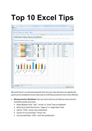
1. Top 10 Excel Tips
Microsoft Excel is an extremely powerful tool, but just a few shortcuts can significantly
speed up the completion of your daily task list and help you become even more effective.
1. Moving around a Worksheet: Here are some shortcuts to help you move around a
worksheet quickly and easily.
 Move Between Cells: “tab”, “arrow” or “enter” keys on keyboard
 Move Up or Down One Screen: “page up” or “page down” keys
 Cell A1: “CTRL + home” key combination
 Column A in Current Row: “home” key
 Last Cell with Data: “CTRL + end” key combination

2. 2. Selecting Cells, Columns and Rows: Selecting items allows you to format text, move or
copy text, and delete large amounts of text at one time. Here are some tips on selecting
cells, columns and rows.
 A Single Cell: Click in cell
 A Single Column: Click on the column letter
 A Single Row: Click on the row number
 The Entire Worksheet: “CTRL + A” key combination or click on the gray box to the left
of the column A and above the Row 1
 Many Cells: Click and drag to select cells when the mouse looks like a white plus sign
3. Using Shortcut Keys: Shortcut keys can drastically reduce the time it takes to edit and
amend an Excel worksheet.
 F5: Displays “Go To” box
 “Shift + F2”: Allows you to edit the cell
 “Ctrl + A”: Select All command
 “Ctrl + B”: Bold command
 “Ctrl + C”: Copy command
 “Ctrl + I”: Italics command
 “Ctrl + V”: Paste command
 “Ctrl + X”: Cut command
 “Ctrl + Z”: Undoes last action/command
 “Ctrl + Shift + ‘”: Applies general number formatting (great for years – 1990, etc)
 “Ctrl + Shift + 1”: Applies number format with 2 decimal places
 “Ctrl + Shift + 2”: Applies time format
 “Ctrl + Shift + 3”: Applies date format
 “Ctrl + Shift + 4”: Applies currency format
4. Using AutoFill: Excel makes it easy for you to quickly complete a series of data, such as
days of the week, month of the year, etc.
 Type in the first part of the series in the cell you would like to begin with (for
example, “January” or “Monday”).
 Move the mouse to the bottom right of cell until it looks like a black plus sign (+).
 Click and drag down the cells to use AutoFill to complete the series. Excel will
automatically fill in the remaining months (February, March, etc) or days of the week
(Tuesday, Wednesday, etc).
5. Keeping Titles in View by Freezing Panes: Have you ever created a larger spreadsheet
with headings in Row 1 and a large list of data below it? If so, you know it can be difficult
to scroll through the large spreadsheet and remember the name of each heading. You
can “freeze” the top row (or column) while you scroll through the spreadsheet.

3.  To freeze the top Row, click in Cell A2.
 Click on “Windows, freeze panes” or “view, freeze panes.”
 Now when you scroll down the spreadsheet, Row 1 will still be visible.
6. Wrapping Text in a Cell: You can modify text in a cell so that it displays on multiple lines
within the cell. There are two different ways to wrap text in a cell.
 Option 1: Click “Format, Cells, Alignment” and select “Wrap Text.”
 Option 2: Select a cell and use “Alt + Enter.”
7. Using Absolute References: When copying formulas, there can choose which of two
reference types you want to use.
 Relative Reference: A cell reference that changes and adjusts to the new cell
location. For example, if you have a formula =A1+B1 and copy it down a column, the
next formula will be =A2+B2, =A3+B3, etc.
 Absolute Reference: A cell reference that does not change or adjust to a new cell
location. For example – if you have a formula =A1*M23 and you want A2 to be
multiplied by M23, then A3 multiplied by M23, you would use absolute referencing.
To make the reference absolute, use dollar signs, so $M$23. =A1*$M$23. When you
copy this down the column, it will now look like: =A2*$M$23, =A3*$M$23, etc.
8. Customizing the Default Workbook: A default workbook can save you time if you
consistently use worksheets with similar layouts. To create a new default workbook,
simply customize a new worksheet and save it as a template.
 Creating a New Template: You can create your own Excel template very easily. First,
create and design the document you would like to make into a template by following
these steps:
1. Once the document in completed, click on “File, Save As.”
2. When the “save as: box opens, change the “save as type” to “Excel
template”. Be sure not to change the location or the folder.
3. Name the template and click “Save.”
 Opening a New Template: Once you have created a new template, you need to
understand how to open and use the new template.
1. Click on “file, new.”
2. Click on the “general” tab or select “my templates . . .”
3. Double click on the template to open.
9. Using the Auto Feature to Automate Processes
To quickly add or average a row or column of data, you can use the “auto” feature. To use
the “auto” feature, highlight a row or column of text and click on the “sum” (∑) button in the

4. upper right-hand corner of the worksheet. You can also select additional functions with the
“auto” feature, by clicking on the down arrow next to the “sum” (∑) button.
10. Moving the Cell Pointer after Entering Data in a Cell:
When you hit the “enter” key in Excel, you will automatically drop down a cell. However,
you can change this default as well as turn off this feature.
 Click on “tools, options.”
 Select the “edit” tab.
 Under “move selection after enter,” you can either select a different direction for
the drop down box, or remove the “check” in front of the option. If you remove the
“check” mark, the “enter” key will not move you to another cell. You will need to use
the arrow keys to move around.