This paper undertakes a Generalized Input-Output analysis on the Swiss economy in order to identify key sectors in greenhouse gases (GHG) emissions. The analysis reveals the actual relevant sectors by taking into account indirect emissions. In order to refine results on key sectors, a sectoral calculation of GHG embodied in Swiss trade is undertaken. Results reveal that some sectors such as food products, machinery rentals and basic metals play an unexpected role in GHG emissions.
Enjoy Night ≽ 8448380779 ≼ Call Girls In Gurgaon Sector 47 (Gurgaon)
Key Sectors in greenhouse gases emissions in Switzerland: An input-output approach
1. Key sectors in greenhouse gases emissions in Switzerland:
An input-output approach
Etienne Jodar*
June 2011
Abstract
This paper undertakes a Generalized Input-Output analysis on the Swiss economy in order to
identify key sectors in greenhouse gases (GHG) emissions. The analysis reveals the actual
relevant sectors by taking into account indirect emissions. In order to refine results on key
sectors, a sectoral calculation of GHG embodied in Swiss trade is undertaken. Results reveal
that some sectors such as food products, machinery rentals and basic metals play an
unexpected role in GHG emissions.
Keywords: embodied emissions; greenhouse gases; input-output; key sectors; Switzerland.
JEL codes: D57, F18, Q53.
*Student in applied economics at the Autonomous University of Barcelona.
2. E.Jodar(2011) 2
1. Introduction
Greenhouse gases (GHG) have received increasing attention in the last decades because of its
role in global warming. Since the beginning of the Industrial Revolution, the burning of fossil
fuels has contributed to an increase of GHG concentration in the atmosphere. As a result, the
greenhouse effect has progressively intensified, leading to global warming and consequent
climate change.
Global warming itself is seen as a major issue for the health of our planet and next
generations. Indeed, climate change, together with global warming, have already harmed
many populations through floods, droughts, increased sea level, melting of ice caps and
natural disasters. The increase in intensity and frequency of these changes is seen by scientists
as a consequence of global warming, which is in turn explained by the amount of GHG
accumulated in the atmosphere (IPCC, 2007).
Thus, in the last decades, mitigation of GHG emissions has become one of the hottest issues
in sustainable development and is in the agendas of most decision makers of each country.
Nations from all around the world have recognized the issue of emissions but do not have
incentives to act alone since it is a global problem. The problem of GHG emissions has
reached such proportions that an international protocol was designed in Kyoto, Japan in a
collaborative, multi-state effort to mitigate GHG. This Protocol was initially adopted on
December 11, 1997 and today 192 countries have signed and ratified this agreement which
entered into force on February 16, 2005.
Concerning the sources of pollution, a field of research has tried to identify, since the end of
the eighties, which industries are the biggest contributors to GHG emissions within a
determinate national economy.
In Switzerland, plenty of studies have inventoried GHG emissions and evaluated trends dating
back to 1990. Indeed, Switzerland has taken this matter as a central issue with periodic reports
on GHG releases published by the Swiss Federal Office of Environment. Some studies have
identified emissions from isolated activities while others have assessed impacts of reducing
the use of some energy types (Werner et al., 2006; Siller et al., 2007; Hartmann et al., 2008;
Perch-Nielsen et al., 2010). However, not much has been done at a macroeconomic level with
the aim of attributing responsibility of GHG emissions towards the diverse sectors of the
Swiss economy. An scattered attempt to do so has been undertaken by the Swiss Federal
3. E.Jodar(2011) 3
Office of Statistics (SFOS) together with the Swiss Federal Office of Environment with a
study published in 2005 (SFOS, 2005). This study analyses GHG emissions by economic
branches using the NAMEA (National Accounting Matrix including Environmental
Accounts) data to assign responsibility of various pollutants to the different sectors of the
economy. 1
Although such studies have been very enlightening in assessing highly polluting activities in
the Swiss economy, some knowledge gaps still remain concerning classification of relevant
sectors within the Swiss economy. Indeed, nothing has been done to assess key sectors with a
vertically integrated economy concern; that is, taking into account indirect GHG emissions
from each economic sector (emissions that are not actually emitted but rather induced). No
study has assessed key sectors in GHG emissions using an Input–Output (IO) framework
which allows seeing linkages between sectors and thus gives a realistic view of the complex
consequences of changes in demand for a determinate product.
The aim of this paper is to assess key sectors in GHG emissions in Switzerland from an
interdependent understanding of the economic sectors. My research question will be: Which
sectors play a key role in GHG emissions in the Swiss economy. My hypothesis is that some
sectors are much more relevant than what is prima facie thought. The knowledge of key
emitter sectors with a concern for indirect emissions is of primary interest in order to achieve
GHG reductions targets. Such new knowledge could help to reduce certain policies that may
seem harmless in emitting GHG but actually pose a threat to the environment (such as
policies that promote the development of a determinate industry).
In order to answer my research question and test my hypothesis, I will use a Generalized IO
model to see how linked in terms of GHG emissions are the different sectors of the Swiss
economy. The magnitude of this linkage will serve me as a proxy of relevance. I will
undertake an IO analysis to trace backward (and forward) the total GHG emissions “needed”
in order for every single sector to produce one more unit of its product. Results will give me
the relevance of each sector. Such an approach will be based on a pioneering paper written by
Wassily Leontief (1970).
Moreover, in order to improve the results of the IO identification of key sectors, I will utilize
a sector-by-sector description of Switzerland’s international foreign trade in terms of GHG
1
NAMEA is a statistical tool that relates environmental data to economic data. Environmental data is compiled
in such a manner that is compatible with the presentation of economic activities in national accounts. This tool
has first been designed by the Dutch after having been developed by EUROSTAT.
4. E.Jodar(2011) 4
embodied in imports and exports. Indeed, such a depiction will, by means of a simple and
plausible assumption, corroborate the standard key sectors assessment. Such a description will
bring light on the international responsibility that each Swiss economic sector has on GHG
emissions and will help to give a more realistic view of each sector’s relevance.
The rest of the paper will be as follows: Section 2 depicts the literature on the topic; Section 3
presents the data needed for the analysis and the problems encountered; Section 4 presents the
methodological framework; Section 5 answers the central research question by presenting
results and exposes some policy implications that come from them; Section 6 refines results
bringing an extra concern, and Section 7 concludes.
2. Literature Review
The concept of key economic sectors did not emerge in environmental Input-Output (IO)
models. In fact, this concept was born before IO models were adapted for environmental
purposes, in a more general context, in the writings of Rasmussen (1957) and Hirschman
(1958). This concept emerged naturally from comments made on the elements of the famous
inverse matrix of Leontief. Rasmussen realized that the column sum of the “Leontief inverse”
would be a measure of the power of dispersion of each corresponding sector while the row
sum of the matrix would be an index of sensitivity of dispersion. Based on these indices, he
derived the concept of “key industry” for sectors with large indices. Since the power of
dispersion measures how deeply a certain sector relies on the whole system, Rasmussen
considered “natural” to characterize sectors with large indices as key sectors. This influential
concept of identifying key sectors in a certain economy, although far from environmental
concerns was later applied to them and will serve as a starting point for this paper.
Later Hazari (1970), in an empirical work on the Indian economy, brought a plus in the
framework of Rasmussen’s linkages. In order to identify key sectors, he chose to weight
Rasmussen’s indices (that would later commonly be called multipliers) to the relative
magnitude of sectors’ deliveries to final demand. He considered that in order to bring out the
relative importance of each sector in the national economy, multipliers had to be weighted.
Since its introduction, this weighted classification of relevant sectors has repeatedly been used
and will be implemented in the present paper.
Later on, Jones (1976), in a classic and seminal paper, brought some clarification on the
matrices that should be employed to accurately measure forward linkages. Basically, he stated
5. E.Jodar(2011) 5
that the matrix used to calculate forward linkages ought to be the “output inverse” (which is
the basic matrix in the supply-driven model founded by Ghosh) instead of the Leontief
inverse, which was used since Rasmussen. From that point in time, there has been a general
approval among regional economists to use the row sum of that matrix in order to assess
forward connectedness between sectors. Here too, the subsequent assessment of key sectors
will follow Jones’ recommendation.
Later on the history of linkages between sectors, and still with the aim of identifying key
sectors, a concern rose in order to calculate “total” linkage of a determinate sector and not
only backward or forward connectedness. As a result, the approach of “hypothetical
extraction” has been developed by various authors such as Cella (1984), among others. This
approach consists on evaluating the relevance of a sector by calculating the total production
that would be achieved without it. Practically, this method consists of removing (or replacing
by zeros) from the matrix of technical coefficient, the row and column of each sector to see
how the production varies without a definite sector. Although this is also used in some
empirical studies, I will not follow this methodological branch to identify key sectors since it
is not superior and requires more formalization and much more calculation than the
“classical” method initiated by Rasmussen (1957).
Concerning IO models to account for pollution externalities, the first application has been
initiated by the IO model founder himself: Wassily Leontief. In a first attempt to incorporate
concerns on pollution in a production framework, Leontief (1970) introduced a row showing
the sectoral pollution in his 1936 basic IO framework. Such a model received the name of
augmented model in reference to this additional non-economic row. Although assessing key
sectors on pollution grounds was not Leontief’s aim in this pioneering paper, the combination
of the IO model and sectoral pollution was a first step in attributing pollution to economic
sectors. The augmented Leontief model was widely extended further; indeed, the idea of
adding data to the initial model has deserved many applications. As a result, augmented
models have been implemented in other areas such as energy consumption and employment
and they ended up being called Generalized IO models.
The combination of augmented models à la Leontief with literature on key sectors has
streamed from the years 1970 according to the availability of the data in the countries under
study. This combination permits to assess key sectors no more on production grounds as
before, but on pollution generation concerns. Thus, many authors such as one of the first: Just
(1974) or recently Alcántara (2010) have carried out studies in different countries. The typical
6. E.Jodar(2011) 6
result of combining augmented models to sector classification à la Rasmussen is that
relevance is assigned to sectors that were not considered important at first sight. Indeed, the
IO analysis makes possible to show up the complex effects and impacts of a production
increase in a determinate sector not only on production but also on pollution grounds. For that
reason, I expect this paper to bring light on the relevance in GHG emissions of the sectors of
the Swiss economy. Likewise, I hypothesize that some sectors are more relevant than what is
prima facie thought.
Later, in the nineties, another branch of literature arose with the aim of identifying CO 2
emissions at an over-boundaries level. This literature started by Proops et al. in 1993 and
followed, among others, by Machado et al. (2001), attempted to take into account CO2
embodied in imports and exports to assess the national balance in GHG emissions. Following
that line, Munksgaard and Pedersen (2001) developed, by means of an IO model, the concept
of “trade balance”, which helps to understand flows of embodied GHG in a country’s trade.
Sánchez-Chóliz and Duarte (2004) developed this concept, disaggregating it in a sectoral
manner which reveals each sector’s importance in GHG embodied in trade.
Concerning Swiss studies, much has been done on GHG emissions, however, nothing to date
using a Generalized IO model with a key sector assessment. 2 Thus, a lot is known about
intense activities within Switzerland, and, say, costs of abandoning an energy type to achieve
CO2 targets, but gaps still remain in understanding the influence of one sector over the other.
In 2005, an important study about sectoral GHG releases was published by the Swiss Federal
Office of Statistics (SFOS, 2005). This publication, based on the estimation of a NAMEA for
the year 2002, has helped to recover the idea of key playing actors in GHG emissions.
Although honorable (since pioneering for Switzerland), this study fails to consider indirect
emissions from economic sectors. Indeed, the assessment of sectors with large shares of
national pollution releases is based only on direct emissions. In addition to that limitation, the
aforementioned study did not offer a high level of disaggregation of the economy that would
allow for accurate policy interventions. Thus, the purpose of the present paper, namely,
assessing key sectors from an IO perspective, takes its motivation from the incomplete view
on relevant sectors.
2
Indeed, Switzerland does not have a long history in estimating IO tables. This lack is twofold. First because of
missing important data and second due to lack of political pressure for compilation of IO tables. Thus, the first
trustworthy table and “sufficiently” disaggregated was released in 2006.
7. E.Jodar(2011) 7
3. Data
The first data set needed for my research is the Input-Output (IO) tables. This set is available
at the SFOS. This set contains 3 tables: a use, a supply and a Symmetric IO Table (SIOT).
Transactions within the economy are disaggregated into 42 sectors and the model is open
with respect to households. The use and supply table come in a squared fashion. Two
packages of data on IO tables corresponding to the years 2001 and 2005 are available. The
following exercise will be based on the latter one. 3
Unfortunately, the data do not provide either an IO table for domestic output or a use table for
imports. Thus, the separation of domestically-produced and imported goods and services
which is of great importance for my analytical purposes is not directly available and a
treatment of the data will be necessary.
Indeed, IO data provided by the SFOS, like some other countries, include imports in the
transaction matrix ( ) in such a way that it is impossible to differentiate if a purchasing sector
is using domestically produced or imported inputs. 4 Data compiled in such a way, that is,
including imports from other countries, is useful if the purpose of a study is to make
comparisons between the structures of production of different countries. However, to analyze
key sectors based on linkages between economic sector, imports must be “scrubbed” since it
is the impact on the domestic economy that is of interest (Miller and Blair, 2009). This
concern has to be taken into account independently of the country, but even more so for a
small country such as Switzerland that has a big foreign trade. In the same line, Jones (1976),
Dietzenbacher et al. (2005), Eurostat (2008) recommend regional economists to infer a
domestic model when data is collected in such a manner. Thus, I operated the data.
The process of inferring a domestic model from a total model (with imports) has commonly
been called “domestication” (Lahr, 2001). My first attempt to net out imports from the
transaction matrix of the SIOT was based on the methodology presented in Miller and Blair
(2009; pp. 150-154). This technique consists of removing imported inputs from the matrix.
When implementing that method to scrub imports, 7 rows of the resultant domestic matrix of
intermediate consumptions ( ) appeared with negative elements. As a consequence, the
domestic direct input coefficient matrix (or technical coefficient matrix), which is essential
to my research, had negative values as well. From an economic point of view this is absurd as
3
A description of sectors is available in the appendix (cf. Table 4).
4
The transaction matrix, matrix of intermediate consumptions or matrix of flows shows the sales and
purchases between sectors.
8. E.Jodar(2011) 8
it means that to engage in production, sectors must release rather than consume inputs from
other sectors.5
In order to overcome that first drawback I looked for other methods to domesticate data
accounting for trade. These other techniques were based on the supply and use tables, not on
as previously mentioned. Thus, I followed Lahr (2001) to obtain domestic technical
coefficient matrices from the use and supply tables. I extrapolated domestic data following
two different techniques proposed by St Louis (1989) and Jackson (1998), respectively. The
former technique assumes implicitly that there are “re-exports” in the export vector (that is,
imports that are exported without processing). The latter assumes no re-exports at all. Both
ways of domesticating the data gave matrices exempt of negative values. I chose to retain
Jackson’s method of domesticating and the subjacent assumption that goes with it since the
export vector given by the use table should not, in principle, include re-exports.
The domestic direct input coefficient matrix ( ) obtained following Jackson’s (1998)
procedure assumes an Industry Based Technology (IBT). This assumption asserts that sectors
have only one input mix in producing different types of commodities. This assumption is
opposed to the Commodity Based Technology (CBT) which assumes that commodities are
produced with the same input structure irrespective of the sector where they are produced.
Although the CBT seems more realistic, I chose to retain the IBT in order to get the technical
coefficient matrix ( ) that I needed. Indeed, the CBT assumption could have led to negative
elements on the domestic technical coefficient matrix but, as mentioned before, that is
unrealistic from an economic point of view. Consequently, it would have been impossible to
interpret CBT as a demand-driven economic circuit (de Mesnard, 2004).
Another concern rises when “domesticating” the data to get a technical coefficient matrix
from the supply and use tables: the choice between inferring a commodity-by-commodity
table or an industry-by-industry one. Since the GHG vector needed to compute my model is
available by industry I decided to retain the latter feature.6 I, thus, finally got a domestic direct
input coefficient matrix with dimensions industry-by-industry that assumes an IBT.
The second essential data to assess key emitting sectors in a Generalized IO model is the
vector of GHG emissions which I obtained from the SFOS as well. This vector collects, in
CO2 equivalent, sectoral emissions of different greenhouse gases (CO2, N2O, CH4, HFCs,
5
This result comes from the fact that 7 economic sectors, have more imports than domestic production.
6
Moreover, most statistics are available in an industry format (employment, value added generated, etc.) thus,
the technical coefficient matrix could be used for other purposes.
9. E.Jodar(2011) 9
PFCs, SF6). This vector is disaggregated into 42 sectors, which corresponds to the sectors
from the IO tables and represents the total amount of pollution emitted during the year 2005.
These emissions are collected in line with the National Accounting Matrix including
Environmental Accounts (NAMEA) that serves as a basis for European Union countries.
4. Methodological Framework
My approaches to identify key sectors are taken from the abundant literature of linkages and
are based on the inverse matrix of Leontief (or total requirements matrix) and the inverse
matrix of Ghosh (or output inverse). In the first stage of assessing the relevance of a sector, I
will consider the magnitude of its pulling effect. By pulling effect, I mean the backward
dependency of the sector; the necessity of inputs provided by other sectors in order for it to
produce. A sector with a large backward effect will “demand” from other sectors. Such a
sector will induce other sectors to produce inputs for it when expanding its production. From
where, a sector with a large backward linkage will be considered relevant as in Rasmussen
(1956). In order to assess relevance of the various sectors from this demand perspective, I will
use the Leontief “demand-driven” model.
As previously said, I am following the line of the Generalized IO models. The methodology
herein is to convert the inverse matrix of Leontief into a matrix that contains emissions rather
than production worth. Indeed, the Leontief inverse represents production in
monetary terms where each element gives the total (direct and indirect) increase in sector
s production needed for an additional Swiss Franc’s worth of sector s production.
Since it is not the production which is of primary interest in this study, I will convert the
Leontief inverse in a matrix that instead of representing production will show emissions. In
order to do it I will follow a methodology used by Alcántara (2007).
In the following lines, matrices and vectors will appear in bold with capital and normal letters
respectively. The “diagonalization” of a vector will figure with a “hat” and the transposition
of a column vector by a prime.
Define:
. (1)
. (2)
10. E.Jodar(2011) 10
where is the “make matrix”, that is, the supply matrix transposed and is the use matrix.
Any element of the supply matrix represents the amount of commodity produced by
industry while any element of the use matrix represents the amount of commodity
absorbed as an input by industry . Vectors and are total commodity output and total
output of industries respectively.
A total direct input coefficient matrix with dimensions industry-by-industry and IBT can be
calculated following Miller and Blair (2009, p. 193). However, as mentioned previously, a
total technical coefficient matrix is not convenient to assess key sectors. Hence, let
domesticate the data following Jackson’s trade adjustment contribution presented in Lahr
(2001) as:
. (3)
Where (42 x 42) is a domestic technical coefficient matrix adjusted for trade. Letters
are vectors of output, imports and exports by products respectively.
And, from the Leontief demand-driven model:
(4)
with the identity matrix, the final demand and the production we get the total
requirement matrix necessary for our analysis which relates changes in demand to
changes in production. As suggested by Jones (1976), the column sum of this matrix should
be used to represent direct plus indirect backward linkages.
Another approach, taken from the Ghosh model developed in 1958, is often used to identify
key sectors. In that year, Ghosh proposed with the same data needed for the Leontief model,
an input-output model with a supply approach. This “supply-driven” model relates sectoral
gross production to primary inputs by the output inverse matrix.7Any element of this matrix
gives in a single number the total production that sector has to do in order to exhaust an
initial increase from one Swiss Franc’s worth of production from sector . The Ghosh inverse
matrix can be calculated from the matrix of intermediate consumptions or extrapolated from
the Leontief inverse following Miller and Blair (2009, p. 548). The difference between these
two matrices (Ghosh and Leontief) is that the Leontief inverse matrix starts at the end of the
production process, with an increase in final demand, and traces the effect backward through
7
Primary inputs are collected within the value added vector which represents labor and capital that economic
branches need, beside the inputs from other industries, in order to produce.
11. E.Jodar(2011) 11
the system while the Ghosh inverse starts at the beginning of the production process, with an
increase in primary inputs, and traces the effect forward through the system.
Thus, in the second stage of identifying key sectors, I will use the supply-driven model of
Ghosh. The approach consists in considering a sector to be “important” if its pushing effect is
relevant. By pushing effect, I mean the capacity of a sector to induce other sectors to produce
(by making them exhaust its output). The strength of that effect will directly depend on the
forward connectedness of sectors. In order to assess what sectors have a high forward linkage,
I will use the row sum of the output inverse as suggested by Jones in 1976.
Extrapolating from the Leontief inverse (as in Miller and Blair, 2009, p. 548) we find the
Ghosh inverse that will allow for assessment of key sectors in a supply
perspective.
Let write the Ghosh supply-driven model (where is not the one from equation 2 and 3) as:
8 (5)
Introduce (42x1), the vector of emissions measured in tons of CO2 equivalent (GHG). Let
be the vector (42x1) of production measured in million of Swiss Francs (CHF). Then,
is a row vector of emission coefficients with units: tons of GHG by millions of
CHF of production. From the previous equation we can deduce that,
. (6)
Let now rewrite the well known Leontief model.
. (7)
Substituting (in equation 6) by its value in the Leontief model, we get:
. (8)
Define:
. (9)
Then
. (10)
8
Where is the vector of value added from the use table which will be called “primary inputs”.
12. E.Jodar(2011) 12
The last equation is a converted Leontief model which instead of connecting the final demand
to production relates it to emissions. The matrix is fundamental in evaluating key sectors in
GHG emissions and therefore to test my hypothesis. Any element of gives the GHG
emissions of sector , needed, to sustain an additional unit of product . Thus, if we sum the
elements of column we will get a multiplier effect of a marginal increase in final demand for
sector j ;Column sum of is therefore a measure of backward linkage on emissions.
Formally, with a summation vector will give the output multipliers for the 42
sectors; the sectoral backward linkage.
Several weights can be applied for bringing out the relative importance of the various sectors
in the national economy. Let weight multipliers according to the greater or lower relevance of
sectors in the final demand, as in Hazari (1970), since unweighted multipliers are potential,
not effective multipliers. Define as a vector of weighted final demands such that .
Thus, will represent the weighted output multipliers.
In order to get an accurate measure of each sector’s backward dependence to the “rest” of the
economy, the on-diagonal elements of should be omitted because it represents internal
linkages (Miller and Blair, 2009, p. 577).9 Thus, let net out from the summation the on-
diagonal elements of splitting between pure an own backward effects corresponding to
external and internal linkages respectively. Following Alcántara’s procedure (2010), let leave
the matrix notation for a little while:
. (11)
. (12)
The methodology for assessing forward linkages is in the same vein. Let post-multiply the
Ghosh model from equation (5) by the emission coefficient vector to get as left-hand side
variable emissions rather than production worth.
. (13)
Define:
. (14)
Then,
9
Those internal linkages are seen as “own-consumption” by sectors.
13. E.Jodar(2011) 13
. (15)
The last equation is a converted Ghosh model. Instead of connecting primary inputs to
production, it relates primary inputs to emissions. Any element of gives the GHG
emissions of sector , needed, to exhaust the additional unit of . Thus, if we sum the elements
of row , we will get a multiplier effect of a marginal increase in primary inputs of sector ;
Row sum of is therefore a measure of forward linkage on emissions. Formally,
with a summation vector will give the supply multipliers for the 42 sectors; the sectoral
forward linkage.
Several weights can be applied for bringing out the relative importance of the various sectors
in the national economy. Herein multipliers will be weighted according to the share of
primary inputs needed for production of the different economic branches. Define as the
vector of weighted primary inputs such that . Thus, will represent the
weighted supply multipliers. As with the demand model, in order to get an accurate measure
of each sector’s forward linkage to the “rest” of the economy, we can separate the sectoral
internal linkages that are located on the on-diagonal elements of matrix
Leaving the matrix notation for a little while:
. (16)
. (17)
Let now categorize sectors into 4 groups according to the relative strength of their linkages. A
simple way to do so is by comparing each weighted multiplier to the average weighted
multiplier. Define the average weighted multiplier as:
. (18)
With this benchmark, let classify sectors following Table 1 (cf. Appendix).
Other taxonomies will be useful to assess backward and forward linkages in more detail,
separating for pure and own linkages. This distinction is useful in terms of policy implication
as will be seen in the following section. Let, thus, categorize sectors into 4 groups according
to their own and pure backward/forward linkages as in table 2 and 3 (cf. Appendix). The
multipliers will be compared with respect to each effect’s (own and pure) specific average.
14. E.Jodar(2011) 14
5. Results
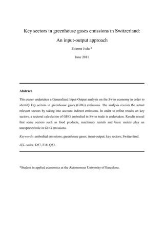
Figure 1 presents results on key sectors in GHG emissions in Switzerland for the year 2005.
Weighted multipliers reveal that 15 sectors are key in a demand side perspective, 14 in a
supply side perspective and 10 sectors out of the 42 are key from both a demand- and a
supply-side perspective. Thus, the IO analysis implemented to emissions reveal that both-
perspective key sectors (“two-side”) in total CO2 equivalent are products of agriculture,
forestry and fishing (1), coke, refined petroleum products (10), other non-metallic mineral
products (12), construction work (24), wholesale trade and commission trade services (26),
transport services (28), public administration and defense services, compulsory social security
services (37), education services (38), health and social work services (39) and sewage and
refuse disposal services (40). 10
0.008
1
0.007 28
0.006 26 40
34
0.005
Supply side
0.004
12
0.003 37
31 24 10
0.002
30 23 38 39
33 27 3
0.001
13 15
0
0 0.001 0.002 0.003 0.004 0.005 0.006 0.007 0.008
Demand side
Figure 1 Key Sectors in GHG Emissions.
Note: This figure classifies the 42 sectors of the Swiss economy into 4 groups according to each sector’s weighted multipliers
of converted demand and supply-driven model. The vertical and horizontal axes show the average weighted multipliers of the
demand and supply-driven model respectively and divide the plane into four regions. The first quadrant presents key sectors
in GHG emissions from both a demand and a supply-driven model. The second quadrant shows key sectors from a supply-
driven model exclusively while the fourth quadrant presents them from a demand-driven model exclusively.
10
Without weighting multipliers by their relative importance in the economy results are totally different. Thus, if
we assume that all sectors are equally important only five sectors are “key” from both perspectives and the sector
of sewage (40) has a humongous effect. This result shows the importance of bringing out every sector’s relative
importance in the economy. In light of that result all following assessments in this work will be weighted.
15. E.Jodar(2011) 15
This first outlook on the 10 two-side key sectors is not very surprising since these sectors
were already known to be serious polluters. The most startling result might be the wholesale
trade sector (26) that is in the top 4 two-side key sectors though it is considered not “that”
relevant in GHG emissions data (cf. Appendix, Table 5).
Notice from Figure 1 that although not relevant from a supply-side analysis, sector 3, namely
food products, is highly relevant from a demand-side perspective and thus deserves attention.
Indeed, when we look at the data (cf. Table 5), sector 3 does not appear to be a big polluter.
Similarly, sector 34, that is, renting of machinery and equipment, is relevant from a supply-
side analysis but not from a demand-side.
Let now analyze in detail backward and forward linkages, distinguishing between own and
pure effects. Such a separation will help to understand why some sectors are relevant in the
IO analysis though not appearing so in the data on direct emissions. Furthermore, such an
analysis is of primary interest in order to fight cleverly against GHG emissions. Indeed, in
terms of policy implications, branches with large own backward linkage must be treated
differently from those with high pure backward linkage. The underlying reason for it is that
sectors with high own linkages exclusively pollute themselves while sectors with large pure
linkage do not pollute much but require others to pollute. Consequently, the policy
implications will have to be different. Results are presented in Figures 2 and 3.
Backward Linkages
A quick outlook on Figure 2 is sufficient to see that sectors with high backward linkage can
behave following really different patterns. A fascinating example is given by sectors 3 and 10
that are similar in the key sector assessment (Figure 1) but are driven by two different forces.
Accordingly, two groups with different policy implications appear from Figure 2. The first is
composed of sectors 1, 28, 40 and exhibits high direct effects (own) but low pulling effects
(pure) upon other sectors. Hence, a strategic policy should aim at adopting measures to reduce
GHG emissions, especially on these sectors. This can be done, for instance, by forcing them
to adopt better technologies. The second group is composed of sectors 3 and 24 and exhibits
substantial indirect effects. This group has to be treated differently from the first group
aforementioned. Here, better technologies do not matter so much since the final polluter is
neither sector 3 nor sector 24; these sectors are not directly responsible for GHG emissions. If
a decision maker wants to mitigate GHG emissions due to these sectors, he should either
16. E.Jodar(2011) 16
mitigate their demand with a tax or focus on the sectors they demand inputs from in order to
make them adopt better technologies.
0.006
3
0.005
0.004
Pure Backward
0.003 24
10
0.002
27 26
15
39
18 33
0.001 37
38 28
13
0 12 40 1
0 0.001 0.002 0.003 0.004 0.005 0.006
Own Backward
Figure 2 Backward Effects.
Note: This figure classifies the 42 sectors of the Swiss economy into 4 groups according to each sector’s weighted multipliers
of own and pure backward linkage. The vertical and horizontal axes show the average weighted multiplier for the own and
pure backward effects respectively and divide the plane into four regions. The pure backward multiplier consists in the
column sum of the F matrix netted out from the on-diagonal element. The own backward is measured by the on-diagonal
element of the matrix and represents internal linkages. The first quadrant presents relevant sectors in GHG emissions for both
own and pure backward effects. The second quadrant shows relevant sectors in pure backward linkage, that is, to the rest of
the economy while the fourth quadrant presents them from an own effect consideration exclusively.
Forward Linkages
An illustrated insight is given by Figure 3. Here again, the results are enlightening. A
decomposition of the forward effects between own and pure forward unveil the grounds for a
sector to be relevant from an IO analysis. Sector 1, 28 and 40 are relevant in GHG emissions
because of their own effects while sectors 26 and 34 and, in a lesser extent, sector 31 appear
relevant because their production will make others to pollute by providing them inputs.
Strategic policy implications to reduce GHG emissions in sectors 1, 28, and 40, here again,
should focus on the adoption of cleaner technologies. Policy implications for sectors 26 and
34 are as follow. On the one hand, their production should be mitigated (for example via a
tax). Indeed, since their relevance in GHG emissions come from other economic sectors,
measures to reduce their production will achieve GHG reduction in other sectors. On the other
17. E.Jodar(2011) 17
hand, policy interventions should focus on sectors that use their output as inputs in order to
make them adopt better technologies. 11
0.005
34
0.004
26
Pure Forward
0.003
31
0.002
37
25 24
0.001
28
10
1
12 40
0
0 0.001 0.002 0.003 0.004 0.005 0.006 0.007 0.008
Own Forward
Figure 3 Forward Effects.
Note: This figure classifies the 42 sectors of the Swiss economy into 4 groups according to each sector’s weighted multipliers
of own and pure forward linkage. The vertical and horizontal axes show the average weighted multiplier for the own and pure
forward effects respectively and divide the plane into four regions. The pure forward multiplier consists in the row sum of the
H matrix netted out from the on-diagonal element. The own forward is measured by the on-diagonal element of the matrix
and represents internal linkages. The first quadrant presents relevant sectors in GHG emissions for both own and pure
forward effects. The second quadrant shows relevant sectors in pure forward linkage, that is, to the rest of the economy while
the fourth quadrant presents them from an own effect consideration exclusively.
Contribution from the IO analysis
Some sectors appear to be much more relevant in GHG emissions than what is commonly
thought; what is shown by data on sectoral emissions. Such a feature is in line with the
hypothesis of the present paper that certain branches have a role in GHG emissions that is not
visible just with data on sectoral emissions and that is highlighted by an IO analysis. The
main result of the papers is the following: some sectors are much more relevant in GHG
emissions than what is prima facie thought. Indeed, certain sectors strongly pull/push others
11
A policy that mitigates demand for sector 1, 28 and 40 has evidently also a positive effect on GHG emissions
mitigation. The logical reason for it is that demand of other sectors for, say, transport services (28) leads to a
substantial increase in transport services from the transport services sector itself. The underlying assumption to
focus on a policy that aims at revising the sector’s technology is that it is considered as more effective.
18. E.Jodar(2011) 18
to pollute while they are considered to be harmless from what is recorded in the data. Thus,
some sectors deserve several comments.
Sectors 3 and 34, namely food products and machinery rentals respectively are representative
of the apparent harmlessness issue. On the one hand, sector 34 does not appear in the top ten
emitting sectors revealed by NAMEA data (cf. Table 5), indeed, its emissions are not that
important compared to other sectors on the top of the list. On the other hand, this sector has a
strong indirect effect on other sectors from a supply perspective. Consequently, it could be
easy to override this sector in a policy that aims at reducing GHG emissions.
Sector 3 is also of particular interest. Its supply dependence is quite substantial, thus pulling
many sectors to pollute when it expands its production. However, surprisingly, its ranking in
the most harming sectors for GHG emissions stands in the ninth position (cf. Table 5).
To give a taste of what these results mean, let us have an example. Using our IO framework,
let imagine a 1% increase in final demand (=1% increase in GDP). Let first imagine that this
increase is due exclusively to an increase in wholesale trade services demand (26) in a way
that all other sectors remain with the same demand. Formally:
. (19)
Using the augmented Leontief model to analyze the impact of that demand change, it comes
out that this 1% increased GDP concentrated in sector 26 will increase GHG emissions by
0.66%.
Let us now contrast this with an equal 1% GDP increase now exclusively due to the food
products sector (3), say, because of an increase in exported Swiss products such as cheese,
chocolate, etc. Let us look at the impact on GHG emissions that would follow in the Swiss
economy. Using the augmented Leontief model to assess the environmental impact of this
different growth path, it comes out that this 1% increased GDP concentrated in sector 3 will
raise GHG emissions by 2.48%.
This result is definitely striking when we consider that sector 26 emits almost twice as much
as sector 3 according to public data (c.f Table 5).
In the same vein, but with the augmented supply-driven model à la Ghosh, let show how an
expansion of primary inputs in sector 34 is relevant. Let imagine a 1% increase in GDP
measured by the value added. Consider in a first stage that this increase in “primary inputs” is
19. E.Jodar(2011) 19
concentrated exclusively in sector 24, say, because of an inflow of immigrant workers.
Formally,
. (20)
Using the augmented Ghosh model to calculate the impact of this change, it comes out that
this 1% increased GDP concentrated in sector 24 will increase GHG emissions by 0.64%. Let
now imagine the same increase in GDP (1%) but now due exclusively to more primary inputs
entering in sector 34. The environmental consequence will be that this 1% increased GDP
concentrated in sector 24 will increase GHG emissions by 1.13%.
These unusual results illustrate the general fact that even though the direct environmental
impact of production from a definite sector can be small, the real-world impact can be large.
This will be the case, particularly, if a sector gets its inputs from activities that pollute a lot.
Thereby, and in order to conclude this section, we see that some sectors that are apparently
harmless to GHG releases are actually more relevant than what is prima facie thought (what is
revealed from public data). Indeed, changes in final demand for commodities and changes in
supply of primary inputs can affect very differently the environment according to the sector
that undergoes the change. 12
6. Refinement of the key sector assessment
An exhaustive concern to assess GHG key sectors in an open economy should take into
consideration imports and exports of goods, services and inputs. Indeed, a country could
avoid pollution by importing (its imports serving for both the final demand and industries
inputs). Thus, to reach a CO2 target, a country could reduce pollution simply by importing
inputs that would have required substantial emissions (Machado et al. 2001). The subjacent
question of this concern is one of responsibility. Who imputing responsibility for emissions?
The producer or the consumer? A recent literature on this matter distinguishing “CO 2
emissions” from “CO2 responsibility” and was first proposed by Proops et al. (1993). This
literature proposes two principles to attribute responsibility. On the one hand, one could
conceive that only the producer should be hold responsible for GHG emissions. On the other
hand, one could consider that the responsibility should fall on the final consumer.
12
Obviously, those surprising results are subject to the underlying assumptions of both demand and supply-
driven models. The former assumes no input substitution, that is, fixed input coefficient, the latter fixed output
coefficient, that is, if sector double its output, then the sales from to each of the sectors that purchase from
will also be doubled.
20. E.Jodar(2011) 20
One drawback of the “producer responsibility principle” is that it does not differentiate
between emissions to provide goods, services and inputs intended for other countries
(exports) from emissions for domestic demand. In spite of this, the producer principle (or
territorial principle) is the one adopted by the Kyoto agreement. This weakness of the Kyoto
agreement harms exporting countries and forces them to make an extra effort to reach CO 2
targets (Munskgaard and Pedersen, 2001).
In contrast, the “consumer responsibility principle” would impute the responsibility on the
consumer. In our case, Switzerland would be held responsible for the GHG emissions
embodied in its imports. A shortcoming to this approach is that nothing can be done by the
importing country to improve technologies abroad and thus reduce emissions.
The calculation of the ecological footprint of a country varies depending on what principle is
used to calculate total GHG emitted; these two principles lead to different valuation of the
impact of a determinate country on the environment. This concern led Munksgaard and
Pedersen (2001) to introduce the concept of “trade balance” in order to show the difference in
CO2 emissions embodied in total imports and exports.
In order to complement the previous analysis of key sectors in GHG releases within the Swiss
economy (which is the aim of this paper) and to obtain a more realistic view of the ecological
footprint of the 42 industries, I will undertake an IO trade balance calculation for the Swiss
economy. Such an analysis will tell if some sectors that did not get a large relevance in the
previous analysis have actually a deep weight at a global level. Furthermore, in calculating the
aggregated trade balance, that is, the sum of all sectors’ trade balance, I will unveil if
Switzerland is a freeloader of the Kyoto agreement (by importing more “GHG intense” inputs
and goods than exporting). By doing that, I will naturally discover if Switzerland is a winner
or a loser of the Kyoto agreement. A negative trade balance would indicate that the country is
avoiding CO2 releases in some extent by importing. This calculation will follow the basic
methodology of Munksgaard and Pedersen (2001) but detailed in a sectoral disaggregation
following the methodology of Sanchez-Chóliz and Duarte (2004).
Let the trade balance of GHG pollution vector be:
13
. (21)
13
Where and are the total and imported direct input coefficient matrices respectively. The former matrix
is calculated as: while the latter as: . Furthermore, , the vector of imports for final demand has
been computed as: .
21. E.Jodar(2011) 21
Results are shown in Table 2 (cf. Appendix). Negative numbers indicate that sectors are net
importers of GHG from the outside while positive values indicate that sectors export more
GHG than import.
Assuming that not all foreign providers are restrained by GHG targets as, for instance, by the
Kyoto protocol, one should give a “relevance premium” to sectors with negative values in
sight of the GHG leakages that can occur in global accounting. Indeed, in the previous IO
analysis, imports were not taken into account because of the data domestication that was
required to assess key sectors. Consequently, no weight was given to the amount of imports in
the key sector assessment and the “territorial principle” was thus implicit. Nonetheless, if
Swiss imports come from countries that are exempt from GHG releases restrictions
purchasers’ sectors should get a sense of responsibility for the carbon embodied in their
imports. With that additional consideration, let review upward the relevance in GHG
emissions of sector 1; 12; 13 among others.
Sector 13, namely basic metals, is a nice example of the contribution of this calculation.
Indeed, this sector did not show up to be a relevant sector in the previous IO analysis.
However, this sector is known to be harmful on GHG emissions in most countries of the
world. In Switzerland, by substituting domestic production by imports, this sector shifts the
burden of acquiring inputs to other countries. If provider countries register their emissions,
there is no point on blaming sector 13 in Switzerland since no carbon leakage will occur.
Nevertheless, if Switzerland imports basic metal commodities from countries that are exempt
from GHG emissions listing (as could be the case) then, sector 13 should get an “extra
relevance”.
It is worth mentioning that on aggregated terms, Switzerland is not a freeloader of GHG
emissions. Switzerland appears to be a loser of the Kyoto agreement. Thus, in order to
achieve GHG emissions targets, Switzerland has to make an extra effort. 14
The emission coefficient vector is domestic. Thus, this calculation assumes implicitly that provider countries
have the same production technology as Switzerland; the same amount of emission by unit of production.
14
It is worth mentioning that this analysis has the only purpose of informing of the relevance of sectors in a
world economy, key sectors having already been defined in the previous section. If we assume that all countries
that provide Swiss imports signed the Kyoto agreement then they are hold responsible for their emissions and
there is no point in calculating GHG embodied in imports since it has already been accounted on the exporting
country. In contrast, this analysis is of particular interest if the foreign providers of the Swiss economy are not
part of the Kyoto agreement since the emissions are not accounted for by the exporting country. In this case, the
net trade balance calculation helps to give a more realistic view of key sectors that has been lost by
domestication of the data.
22. E.Jodar(2011) 22
Conclusion
The Generalized IO analysis used to assess key sectors in GHG emissions for Switzerland in
2005 shows that some sectors are more relevant than what is commonly thought. Indeed, the
IO analysis has allowed interdependencies between sectors to be taken into account and, thus,
the pulling and pushing effects that occur when a determinate sector increases its production.
Results show that the food products sector (3) and machinery rentals sector (34) present high
indirect effects and are thus not harmless to the environment when their productions increase.
Moreover, a refinement of the key sector assessment has been undertaken by a calculation of
GHG embodied in trade. This refinement has the purpose of recovering a dimension lost by
the domestication of the data needed for the key sector assessment, namely, the concern for
GHG embodied in imports. By assuming that not all foreign Swiss providers have emission
restrictions, an “extra responsibility” has been assigned to sectors that import more GHG than
export. This extension of the key sector assessment shows that some sectors, such as basic
metals (13), among others, should get an extra relevance in order to accurately assess their
responsibility in GHG emissions.
In terms of policy implications, the aforementioned food products sector (3) and machinery
rentals sector (34) should receive a demand and production mitigation policy, respectively.
Indeed, such interventions will achieve deep GHG mitigations in the whole Swiss economy
because these sectors make others to pollute when they expand their production.
Acknowledgments
This work is the outcome of an applied economic master’s dissertation project. I am grateful
to the Swiss Federal Office of Statistics team and Michael Lahr for answering questions as
well as my supervisor Emilio Padilla and Vicent Alcántara for their precious comments. All
errors are mines.
23. E.Jodar(2011) 23
References
Alcántara, Vicent. Pablo del Río and Félix Hernández (2010) “Structural analysis of
electricity consumption by productive sectors. The Spanish case”, Energy, 35, 2088-
2098.
Alcántara, Vicent (2007) “Análisis input-output y medio ambiente: una aplicación a la
determinación de sectores clave en las emisiones de SOx en Catalunya”, Nota
d’economia, nº 87, 1r cuadrimestre.
Cella, Guido (1984) “The Input-Output Measurement of Interindustry Linkages”,
Oxford Bulletin of Economics and Statistics, 46, 73–84.
de Mesnard, Louis (2004) “Understanding the shortcomings of commodity-based
technology in input-output models: An economic-circuit approach”, Journal of
Regional Science, 44, 125-141.
Dietzenbacher, Eric. Vito Albino and Silvana Kühtz (2005) “The Fallacy of Using
US-Type Input-Output Tables”, Paper presented at the 15th International Conference
on Input-Output Techniques, Beijing China, June 27–July 1, 2005.
Eurostat/European Commission (2008) Eurostat Manual of Supply, Use and Input-
Output Tables. Luxembourg: Office for Official Publications of the European
Communities.
Ghosh, Ambica (1958) “Input-Output Approach to an Allocation System”,
Economica, 25, 58–64.
Hartmann, Michael. Robert Huber, Simon Peter and Bernard Lehmann
(2009)”Strategies to mitigate greenhouse gas and nitrogen emissions in the Swiss
agriculture: the application of an integrated sector model ”, IED Working Paper 9.
Hazari, Bharat R. (1970)” Empirical identification of key sectors in the Indian
economy”, The review of economics and statistics, vol 52(3), 301-305.
Hazari, Bharat R. and J. Krishnamurty (1970)”Employment implications of India’s
industrialization: Analysis in an input-output framework”, The review of economics
and statistics, vol 52(2), 181-186.
Hirschman, Albert O. (1958) The Strategy of Economic Development, New Haven,
CT:Yale University Press.
IPCC (2007) Climate Change 2007: Impacts, Adaptation and Vulnerability.
Contribution of Working Group II to the Fourth Assessment Report of the
Intergovernmental Panel on Climate Change, M.L. Parry, O.F. Canziani, J.P.
24. E.Jodar(2011) 24
Palutikof, P.J. van der Linden and C.E.Hanson, Eds., Cambridge University Press,
Cambridge, UK, 976pp.
Jackson, Randall W. (1998) “Regionalizing national commodity-by-industry
accounts”, Economic systems Research, 10, 223-238.
Jones, Leroy P. (1976) “The measurement of Hirschmanian linkages”, Quarterly
Journal of economics, 90, 323–333.
Just, James (1974) “Impacts of New Energy Technology Using Generalized Input-
Output Analysis” in Michael Macrakis (ed.), Energy: Demand Conservation and
Institutional Problems. Cambridge, MA: MIT Press, 113–128.
Lahr, Michael L. (2001)”Reconciling Domestication Techniques, the Notion of Re-
exports and Some Comments on Regional Accounting”, Economic Systems Research,
13, 165-179.
Leontief, Wassily (1970) “Environmental Repercussions and the Economic Structure:
An Input-Output Approach”, Review of Economics and Statistics, 52, 262–271.
Machado, Giovani. Roberto Schaffer and Ernst Worell (2001) “Energy and carbon
embodied in the International Trade of Brazil: an input–output approach”, Ecological
Economics 39, 409–424.
Miller, Ronald E. and Blair, Peter D. (2009) Input–Output Analysis: Foundations and
Extension. 2nd edition. Cambridge University Press.
Munksgaard, Jesper and Klaus A. Pedersen (2001)”CO2 accounts for open economies:
producer or consumer responsibility”, Energy Policy, 29, 327–334.
Perch-Nielsen, Sabine. Ana Sesartic and Matthias Stucki (2010)”The greenhouse gas
intensity of the tourism sector: The case of Switzerland”, Environmental Science &
Policy, 13, 131-140.
Proops, John L.R. Faber, Malte M. and Wagenhals, Gerhard (1993) Reducing CO2
Emissions: A Comparative Input-Output Study for Germany and the UK, Springer,
Berlin.
Rasmussen, Nørregaard P. (1957) Studies in Inter-sectoral Relations. Amsterdam:
North-Holland.
Sánchez-Chóliz, Julio and Rosa Duarte (2004) “CO2 emissions embodied in
international trade: evidence for Spain”, Energy Policy, 32, 1999-2005.
SFOS Commission (2005) “Emissions de gaz à effet de serre par branche économique.
NAMEA pilote pour la Suisse en 2002“, Neuchâtel, 74 pages. Available at:
25. E.Jodar(2011) 25
http://www.bfs.admin.ch/bfs/portal/fr/index/news/publikationen.html?publicationID=2
082
Siller, Thomas. Michael Kost and Dieter Imboden (2007) “Long-term energy savings
and greenhouse gas emission reductions in the Swiss residential sector“, Energy
Policy, 35, 529-539.
St. Louis, Larry V. (1989)”Empirical tests of some semi-survey update procedures
applied to rectangular input-output tables”, Journal of Regional Science, 29, 373- 385.
Werner, Frank. Ruedi Taverna, Peter Hofer and Klaus Riechter (2006) “Greenhouse
gas dynamics of an increased use of wood in buildings in Switzerland“, Climatic
Change, 74, 1-3, 319-347.
26. E.Jodar(2011) 26
Appendix
Table 1 Classification of Sectors.
Forward Linkage
Supply perspective
Irrelevant Sectors
Key Sectors
Backward Linkage Demand
Two-side Key
perspective Key
Sectors
Sectors
Note: Table 1 classifies sectors according to a benchmark which is the average weighted multiplier. The
weighted multiplier is a measure of sectoral connectedness weighted according to the relevance of the sector in
the whole economy. Sectors with high backward linkage exclusively are key in a demand perspective. Sectors
with high forward linkage exclusively are key in a supply perspective. Sectors with both a large backward and
forward linkage are key from both perspectives. Results are shown in Figure 1.
Table 2 Classification of Backward Linkages.
Own Backward
Relevant Sectors in
Irrelevant Sectors own Backward
Pure Backward Linkage
Relevant Sectors in Relevant Sectors in
pure Backward both own and pure
Linkage Backward Linkage
Note: Table 2 takes backward linkages and split them into own and pure backward. Each effect (own and pure)
is compared to its own average. Results are shown in Figure 2.
Table 3 Classification of Forward Linkages.
Own Forward
Relevant Sectors in
Irrelevant Sectors own Forward
Pure Forward Linkages
Relevant Sectors in Relevant Sectors in
pure Forward both own and pure
Linkages Forward Linkages
Note: Table 3 takes forward linkages and split them into own and pure forward. Each effect (own and pure) is
compared to its own average. Results are shown in Figure 3.
27. E.Jodar(2011) 27
Table 4 Sectors of the Swiss Economy.
1 Products of agriculture, forestry and fishing
2 Products of mining and quarrying
3 Food products, beverages and tobacco products
4 Textiles
5 Wearing apparel, furs
6 Leather and leather products
7 Wood and products of wood and cork (except furniture); articles of straw and plaiting materials
8 Pulp, paper and paper products
9 Printed matter and recorded media
10 Coke, refined petroleum products and nuclear fuel; chemicals and chemical products
11 Rubber and plastic products
12 Other non-metallic mineral products
13 Basic metals
14 Fabricated metal products, except machinery and equipment
15 Machinery and equipment n.e.c.
16 Office machinery, computers and electrical machinery n.e.c.
17 Radio, television and communication equipment and apparatus
18 Medical, precision and optical instruments, watches and clocks
19 Motor vehicles, trailers and semi-trailers
20 Other transport equipment
21 Furniture; other manufactured goods n.e.c.
22 Secondary raw materials
Electrical energy, gas, steam, hot water; collected and purified water and distribution services of
23
water
24 Construction work
Trade, maintenance and repair services of motor vehicles and motorcycles; retail sale of automotive
25
fuel
Wholesale trade and commission trade services, except of motor vehicles and motorcycles, Retail
26 trade services, except of motor vehicles and motorcycles; repair services of personal and household
goods
27 Hotel and restaurant services
28 Transport services
29 Supporting and auxiliary transport services; travel agency services
30 Post and telecommunication services
31 Financial intermediation services, except insurance and pension funding services
Insurance and pension funding services, except compulsory social security services (includes also
32
part of CPA 67)
33 Real estate services (incl. private households)
Renting of machinery and equipment without operator and of personal and household goods; other
34
business services
35 Computer and related services
36 Research and development services
37 Public administration and defense services; compulsory social security services
38 Education services
39 Health and social work services
40 Sewage and refuse disposal services, sanitation and similar services
41 Membership organization services n.e.c.; recreational, cultural and sporting services
42 Other services; private households with employed persons
28. Table 5 Ranking of Top Polluters. Table 6 Sectoral Trade Balance.
Ranking of Top Polluters Trade Balance
Position Sector Tons of GHG emissions Sector b
1 1 6435 1 -1761
2 28 5969 2 -101
3 40 5526 3 -48
4 12 3403 4 -69
5 10 2653 5 -70
6 26 1746 6 -46
7 37 1526 7 -92
8 24 1205 8 65
9 3 937
9 7
10 39 933
10 1346
11 27 876
11 26
12 34 803
12 -557
13 23 775
13 -425
14 8 768
14 114
15 7 642
15 126
16 13 628
16 -23
17 30 481
17 -25
18 14 388
18 134
19 15 362
19 -97
20 29 350
20 -10
21 25 295
21 -60
22 31 271
22 -10
23 9 238
24 16 225 23 105
25 41 221 24 14
26 18 206 25 20
27 35 188 26 377
28 11 136 27 -18
29 4 136 28 998
30 38 132 29 76
31 32 128 30 49
32 21 117 31 108
33 17 117 32 14
34 42 116 33 10
35 33 82 34 110
36 2 63 35 11
37 36 59 36 23
38 20 40 37 16
39 22 35 38 19
40 5 23 39 22
41 19 15 40 274
42 6 12 41 -8
42 2
Total 39261
National Balance 644
Note: Sectors are ranked according to their amount
of GHG emissions for the year 2005. Data come Note: This table shows the result of the calculation
from the NAMEA 2005. of equation 21. The trade balance is disaggregated
at a sectoral level. A positive value means that a
definite sector exports more GHG than receive by
its imports from abroad.