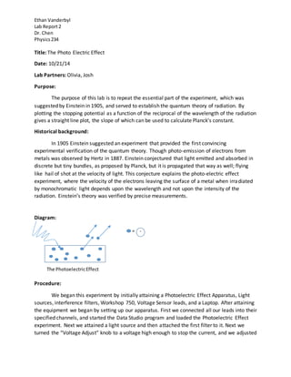
1. Ethan Vanderbyl
Lab Report2
Dr. Chen
Physics234
-
Title: The Photo Electric Effect
Date: 10/21/14
Lab Partners: Olivia, Josh
Purpose:
The purpose of this lab is to repeat the essential part of the experiment, which was
suggested by Einstein in 1905, and served to establish the quantum theory of radiation. By
plotting the stopping potential as a function of the reciprocal of the wavelength of the radiation
gives a straight line plot, the slope of which can be used to calculate Planck’s constant.
Historical background:
In 1905 Einstein suggested an experiment that provided the first convincing
experimental verification of the quantum theory. Though photo-emission of electrons from
metals was observed by Hertz in 1887. Einstein conjectured that light emitted and absorbed in
discrete but tiny bundles, as proposed by Planck, but it is propagated that way as well; flying
like hail of shot at the velocity of light. This conjecture explains the photo-electric effect
experiment, where the velocity of the electrons leaving the surface of a metal when irradiated
by monochromatic light depends upon the wavelength and not upon the intensity of the
radiation. Einstein’s theory was verified by precise measurements.
Diagram:
Procedure:
We began this experiment by initially attaining a Photoelectric Effect Apparatus, Light
sources, interference filters, Workshop 750, Voltage Sensor leads, and a Laptop. After attaining
the equipment we began by setting up our apparatus. First we connected all our leads into their
specified channels, and started the Data Studio program and loaded the Photoelectric Effect
experiment. Next we attained a light source and then attached the first filter to it. Next we
turned the “Voltage Adjust” knob to a voltage high enough to stop the current, and we adjusted
The PhotoelectricEffect
= -

2. Ethan Vanderbyl
Lab Report2
Dr. Chen
Physics234
the “Zero Adjust” so that the analog current meter read zero. Then we turned down the
“Voltage Adjust” knob to its counterclockwise limit, and moved the apparatus or the light
source until the radiation was striking the center of the photodiode aperture. We adjusted the
radiation intensity so that the meter was reading approximately 15 on the scale. After
performing these tasks we turned the “Voltage Adjust” knob up high enough to bring the
current meter down to zero. After doing this we started collecting data in the Data Studio, and
continued to gradually turn down the Voltage Adjust knob on the apparatus. We performed the
same procedure for each filter.
Data:
Results:
Planck’s Constant (m2 kg / s) Calculated Value m (m2 kg / s) % Error
6.62606957 × 10-34 m2 kg / s 4.27 ∗ 10−34 m2 kg / s 36%
Wavelength
(m)
Stopping Potential 1
(V)
Stopping
Potential 2 (V)
4.358E-07 1.211 0.786
0.00000048 0.712 0.79
5.461E-07 0.67 0.624
5.896E-07 0.488 0.583
6.328E-07 0.3 0.358
0.000000765 0.11 0.25
1/Wavelength
(m)
Average Stopping
Potential (V)
2294630.564 0.9985
2083333.333 0.751
1831166.453 0.647
1696065.129 0.5355
1580278.129 0.329
1307189.542 0.18

3. Ethan Vanderbyl
Lab Report2
Dr. Chen
Physics234
Graphs:
λ = 480 nm
y = 8E-07x - 0.9002
0
0.2
0.4
0.6
0.8
1
1.2
0 500000 1000000 1500000 2000000 2500000
AverageStoppingVoltage(V)
1/wavelength (m)
AverageStopping Potentialvs. 1/wavelength

4. Ethan Vanderbyl
Lab Report2
Dr. Chen
Physics234
λ = 589.6 nm
λ = 435.8

5. Ethan Vanderbyl
Lab Report2
Dr. Chen
Physics234
λ = 546.1
λ = 632.8 nm

6. Ethan Vanderbyl
Lab Report2
Dr. Chen
Physics234
λ = 765 nm
Calculations:
1
𝜆
𝑎𝑣𝑒𝑟𝑎𝑔𝑒 𝑠𝑡𝑝 =
𝑠𝑡𝑝1 + 𝑠𝑡𝑝2
2
ℎ = (𝑠𝑙𝑜𝑝𝑒 ∗ 𝑒)/𝑐
% Error =
𝑛𝑣−𝑐𝑣
𝑛𝑣
∅ = 𝑏𝑒
𝐸 = ∅
Example Calculations:
1
𝜆
=
1
5.46E − 07
𝑎𝑣𝑒𝑟𝑎𝑔𝑒 𝑠𝑡𝑝 =
. 912 + .94
2
= .926
ℎ =
((8∗10−7)(1.60217657∗10−19
𝑐𝑜𝑢𝑙𝑜𝑚𝑏𝑠))
(3∗
108 𝑚
𝑠
)
= 4.27 ∗ 10−34
% 𝐸𝑟𝑟𝑜𝑟 =
(6.62606957 × 10−34
) − (4.27 ∗ 10−34)
(6.62606957∗ 10^ − 34)
= 36%

7. Ethan Vanderbyl
Lab Report2
Dr. Chen
Physics234
∅ = .9002 ∗ (1.60217657 ∗ 10−19) = 1.44227935 ∗ 10−19 𝐽
𝐸 = 1.44227935 ∗ 10−19 𝐽
Questions:
1. The point at which the best-fit line intersects the x-axis is where the stopping average
stopping voltage is 0. The wavelength at this point is equal 888nm, which was solved by using
the equation for the best-fit line. The Energy at this point is 1.44227935 ∗ 10−19
𝐽.
2. When the best-fit line intersects the y-axis the wavelength is going to infinite because of the
relationship: 1/wavelength, and the average stopping potential is negative. Once the
wavelength goes beyond 888nm there is no electron emission off the metal.
Conclusion:
In conclusion we were able to accomplish the purpose of this lab by plotting the
stopping potential as a function of the reciprocal of the wavelength of the radiation which gives
a straight line plot, in which we can use the slope to calculate Planck’s constant. Our data
verifies the validity of our experiment because we attained a 36% error, which is acceptable in
this case. The first graph presented in this data set is the graph of average stopping potential vs.
one over wavelength. This graph is in fact our solution which we used to calculate Planck’s
constant. The linear tread line gave us the slope of the line, which we then plugged into the
equation: ℎ = (𝑠𝑙𝑜𝑝𝑒 ∗ 𝑒)/𝑐 , and an error of 36%. We also used the equation of this line to
solve for the x-intercept, which gave us the value of the wavelength to be 888nm. Though this
value has some relative error it does make sense to attain this value because once the
wavelength is too large light will no longer be an electron emission off the metal. The following
graphs are graphs of the trials for each wavelength of light, and allowed use to attain our
calculated Planck’s constant by determining the average stopping potential for each
wavelength and plotting the average stopping potential versus 1/wavelength. Once again we
accomplished our purpose because we attained an acceptable error of 36%.
In this experiment our major sources of error were due many different factors, some of
which included: restraints on the Voltage sensor, restraints on the actual apparatus, and faulty
averages of the stopping potential. A few things that could have improved this experiment
include: improved instrumentation, improved analysis of each stopping potential, and an over
improvement of the apparatus. Each of these improvements we reduce our percent error,
giving us a more accurate calculation of Planck’s constant.