1. Dylan Skusek
SeoJin Lee
3/19/2015
Racial Diversity of a State and its Effects of Racial Adversity variables.
It was nearly 70 years ago that the Civil Rights movement swept the United States of
America in hopes of procuring equality for not only Africans, but for all other minorities. And
while the U.S. has made great strides in its quest for equality for all, it still faces equality issues
today. The purpose of this paper is to delve deeper into the subject; specifically, the following
hypothesis will be tested: That the racial adversity a person faces does not have an effect on their
income. And on a larger scale, that the diversity of a state has no effect on its mean income (this
will be a comparison of a two states and thus a simple comparison). By the previously mentioned
statement we mean to talk about the person’s social makeup; we want to see how the income of a
born and raised white “American” stands up to that of an immigrant or minority. For brevities
sake, we will refer to the hypothesis as the following
H0: ξ = θ = ε = λ = β1 = β2 = β3 = β4 = 0,
where the following symbols are our coefficients that are affecting a combination of various
racial adversity variables, and the hypothesis being that they all have no effect on the income of a
person. Our alternative hypothesis would then simply be:
HA: ξ ≠ θ ≠ ε ≠ λ ≠ β1 ≠ β2 ≠ β3 ≠ β4 ≠ 0

2. With the aforementioned hypothesis being such a controversial one, it would help to look
at previous literature to gain an idea of what one can expect the outcome of the hypothesis to be.
The Institute for Policy Studies reports that on average Whites have a median income of
$56,000, a median net worth of $140,000, and approximately 75% of all Whites own their
homes; compared to Blacks, who only have a median income of $37,000, a median net worth of
$22,000, and only 50% own their homes (Inequality.org). Furthermore, the Urban Institute
reports that the racial wealth gap is not improving, but rather has been getting worse, to the point
where Whites on average have wealth 3 times greater than non-whites (Urban.org). Deeper
reading from Christopher Jencks Inequality: A Reassessment of the Effect of Family and
Schooling in America points out that often non-whites often are not able to achieve a higher
earning than Whites due to the inequalities in educational attainment as well as inequality of
occupational status (Jencks). Many more articles can be brought forth to show how in-depth
research has gone into the subject, but the previous examples should suffice. Based on previous
knowledge, it is fair to assume that our hypothesis will end up being rejected.
Now for the exact variables we will be measuring, it is important to take into account any
factors that could also contribute to a individual’s mean income. We will primarily be focusing
on factors of diversity, such as the race of the respondent, their citizen status, English
proficiency, etc. along with some basic variables such as age, sex, and so forth. All in all we will
have 12 independent variables affecting our dependent variable, income. The following variables
will be included in our regression equation, which will look as such:
log(Income) = C + αAGE + γSCHOOL + σMALE + β1BLACK + β2NATIVE + β3ASIAN +
β4OTHER + εLAN + θENTRY + λPOB + τOC + ξENG

3. Where C is our intercept term. ENG is an English proficiency rating on a scale from 0-4
(4 being the worst or no English proficiency at all), BLACK, NATIVE, ASIAN, OTHER are all
race minorities, LAN is the
predominant language of the
respondent/language spoken
at home, ENTRY is when
the respondent emigrated to
the U.S. (0 if they were born
here, +1 for every 20+ years
of having emigrated here),
POB is the place of birth for
the respondent, and OC is a dummy variable where it’s value is = 1 if the respondent is an only
child. The other variables are self-explanatory and are already known to have a significant
impact on one’s income. One issue we might run into is multicollinearity; some of the variables
are somewhat related (English proficiency might be related to the language spoken at home) so
we’ll be sure to check for any correlation between some similar variables. Another issue we need
to look out for is accidentally omitting any variables. While we have a significant amount of
variables to test, there’s always the opportunity for us to omit one that has a significant effect,
thus causing it’s affect to be picked up by another variable and making it biased. To get a general
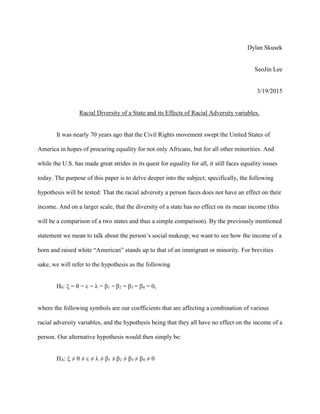
idea of each state’s racial makeup, two histograms for a respondent’s place of birth are
supplemented. If they are native to the United States, they receive a 1. If they were born in

4. Europe, Latin America, or Australia/New Zealand, they
receive a 2. If they were born in Asia, they receive a three.
And if they were born in Africa, they receive a four.
In order to investigate this problem, we will need a
reliable set of data that includes many variables whose
information is gathered nearly simultaneously; as a result,
we will turn to data gathered from the United States Census
Bureau. The data has been acquired from every state during
the 2009-2013 period. In it includes answers to the census
questionnaire, which contains questions relating to every
social aspect of a U.S. citizens life: race, sex, age, location,
children, and so forth. For the sake of simplicity and to avoid complexity, only data from Maine
and Virginia State will used along with a subset of 1,200 samples. We will use these two states
since they are on opposite ends of the racial diversity spectrum, with Maine having the most
homogenous population and Virginia being one of the most diverse. This sharp contrast in
diversity should allow us to see the effect of racial diversity on the mean income. Also, using
states in the same general geographic area and political makeup will allow us to see the near
direct effect of racial variables. On the next page is a quick summary table of some basic
statistics calculated in STATA from a sample size of 1,200 from the census.
During the retrieval of the data, we needed to also clean it as well in order for it to work
with STATA. One example is of the respondent’s place of origin. If they were native, they got a
0. If they were from Europe, Australia/New Zealand, or Latin America, they received a 1. If they
96.41
3.003 .5004 .0834
0
20406080
100
Percent
-1 0 1 2 3
POB
Maine Place of Birth Histogram
89.57
4.837 5.004
.5838
0
20406080
100
Percent
-1 0 1 2 3
POB
Virginia Place of Birth Histogram

5. were from Asia, they received a 2.
And if they were from Africa, they
received a 3. The logic behind this
denotation was that being from
outside the U.S. will have a negative
impact on income, and that the racial
challenges and adversity of a person
from Europe, Australia/New
Zealand, or Latin America would be
less than that of Asia and Africa. Secondly, any income of 0 was increased to 1, so that way
when we take the log of all incomes, the log of a person’s income will be 0. We also flipped
some dummy variables in the census data; females and males, for example, were represented as 2
and 1, respectively. We changed females from 2 to 0, just for simplicity’s sake. One other major
change we made to the data was separating the racial data into separate dummy variables. So a
“2” under our RAC1P data represented a black person, was moved to the dummy variable
“BLACK”. This was done for each race except for whites, who are represented by all race
variables as a 0.
When we are performing our regression for both states, we will do it 2 separate ways:
once with all non-racial variables, and once with all the variables. The reasoning for this is to see
how omitting certain variables can affect our R2
value. The results are shown below in the
STATA and hypothesis testing tables:

8. At first, nothing of interest really seems to come into view. All of our racial adversity
variables, such as ENG, POB, ENTRY, LAN, are all insignificant when a t-test is performed. In
Maine’s regression, however, the t-values of the NATIVE, BLACK, OTHER variables are
significant at the 1% critical value of 2.576 and the 5% critical value of 1.960. Both the NATIVE
and BLACK variables have negative impacts in both equations whereas OTHER positively
increase the log(INCOME) in Maine but decreases it in Virginia’s. When compared to
Virginia’s, none of the racial adversity variables are significant. Virginia’s R2
value barely
changes with the inclusion of the racial adversity variables. However, what else is interesting is
that Maine’s R2
value becomes 0.02 greater (or 2% more of the equation is explained) due to the
inclusion of racial adversity variables. The implication of this will be discussed at the end.
Furthermore our standard variables, like AGE, SCHOOLING, SEX, and OC are all almost
exactly alike between the two states with or without the inclusion of the racial adversity
variables. But how, if at all, are the affecting each other? Are they correlated? Below in our
tables, anything over 15% correlation has been highlighted in blue whereas anything over 50%
correlation is highlighted in purple. Immediately it becomes evident that the English proficiency
variable has issues with
correlation, as well as
our ASIAN, ENTRY,
and POB variables. That
makes sense, since
someone born in another
country and emigrated
here would not be as

9. fluent in English than someone who was born here. We were correct in the beginning to assume
there might be a chance at correlation between these two variables, but included them regardless.
The system of separating people who emigrated from Asia, Europe/Latin America, or Africa
could be flawed and would perhaps deserve dummy variables of their own. Doing so could at
least lessen the severity of correlation between the ENG, POB, and ASIAN variables. We also
look at the F-statistic, which is a measure of getting the regression by chance. It is interesting
that while all the F values for every table are significant, they significantly decrease by more
than 100% at the inclusion of the racial adversity values even though in the Virginia regression
they were insignificant. Finally, there was one effect we accidentally stumbled upon; the OC
variable is significant and has a significant effect on income. The census has data only on
whether the respondent was a single child, and not on the amount of siblings. This could be due
to a mistake in gathering data, where most individuals who are a single child are a young age and
thus would have no income. But it could also be correct due in part that more people in a family
can help each other through tough financial times or support them.
All in all, there are a few implications to take note when looking at the data. We fail to
reject the null hypothesis that ξ = θ = ε = λ = 0, or that racial adversity factors, such as date of
entry into the U.S., place of origin, etc. have no effect on income and we saw no difference in for
this hypothesis in either Maine or Virginia. However, we reject the notion the diversity of state
has no effect on the income of an individual if they are a different race, but only if that state is
significantly homogenous. About 3% of Maine’s population is non-white, and it’s BLACK and
NATIVE variables are both significant and have negative coefficients, and its regression or R2
became 2% more efficient at the inclusion of these variables. Virginia, on the other hand, has a
non-white population of about 36.4%, had no significant racial adversity variables, and the

10. regression did not become more efficient with the inclusion of racial adversity. Thus the take
away from the experiment is that the diversity of a state has an effect on the income of racially
different respondents.

11. Works Cited
- "Racial Inequality | Inequality.org." Inequalityorg. Institute for Policy Studies, n.d.
Web. 15 Mar. 2015.
- "Interactive Race Graphic." The Urban Institute. Association for Public Policy
Analysis and Management, n.d. Web. 19 Mar. 2015.
- Jencks, Christopher. Inequality: A Reassessment of the Effect of Family and
Schooling in America. New York: Basic, 1972. Print.
- United States. United States Department of Commerce. United States Census
Bureau. 2010 Census. Washington, D.C.: U.S. Department of Commerce, Economics
and Statistics Administration, U.S. Census Bureau, 2013. Web.