SlideShare ist ein Scribd-Unternehmen logo
1 von 32
Downloaden Sie, um offline zu lesen
Fluid Mechanics (MEng2113) Lecture Notes
Tsegaye Getachew Alenka
Department of Mechanical Engineering
Wolaita Sodo University
tsegaye.getachew@wsu.edu.et
February 26, 2023
Contents
1 Module Structure 1
2 Properties, Statics, kinematics, Dynamics and Scaling 1
2.1 Primary and Secondary properties . . . . . . . . . . . . . . . . . . . . . . . . . . . . . . . . . . . . . . 1
2.2 Flow Patterns: Stream/streak/pathlines . . . . . . . . . . . . . . . . . . . . . . . . . . . . . . . . . . . 2
2.2.1 Flow Measurement . . . . . . . . . . . . . . . . . . . . . . . . . . . . . . . . . . . . . . . . . . . 3
2.3 Fluid Statics . . . . . . . . . . . . . . . . . . . . . . . . . . . . . . . . . . . . . . . . . . . . . . . . . . 4
2.4 Integral Relations for a Vontrol Volume . . . . . . . . . . . . . . . . . . . . . . . . . . . . . . . . . . . 5
2.4.1 Flow Classification . . . . . . . . . . . . . . . . . . . . . . . . . . . . . . . . . . . . . . . . . . . 5
2.4.2 Flow Analysis . . . . . . . . . . . . . . . . . . . . . . . . . . . . . . . . . . . . . . . . . . . . . . 6
2.4.3 Bernoulli Equation . . . . . . . . . . . . . . . . . . . . . . . . . . . . . . . . . . . . . . . . . . . 7
2.5 Differential Relations for a Fluid Particle . . . . . . . . . . . . . . . . . . . . . . . . . . . . . . . . . . 8
2.5.1 2D Potential Flow Theory . . . . . . . . . . . . . . . . . . . . . . . . . . . . . . . . . . . . . . 9
2.6 Dimensional Analysis and Similitude . . . . . . . . . . . . . . . . . . . . . . . . . . . . . . . . . . . . . 13
2.6.1 Method 1: Exponential Method . . . . . . . . . . . . . . . . . . . . . . . . . . . . . . . . . . . . 14
2.6.2 Method 2 & 1: Control Volume Analysis along with Functional Relation Analysis & Exponent
Method . . . . . . . . . . . . . . . . . . . . . . . . . . . . . . . . . . . . . . . . . . . . . . . . . 15
2.6.3 Common Dimensionless Parameters for Fluid . . . . . . . . . . . . . . . . . . . . . . . . . . . . 16
2.6.4 Method 1: Step-by-Step Approach or Scaling-up Similarity and Model Testing . . . . . . . . . 17
2.7 Review Exercise Part I:Questions A . . . . . . . . . . . . . . . . . . . . . . . . . . . . . . . . . . . . . 18
3 Boundary layer, Compressible and Incompressible Flow, and Losses in Pipe 19
3.1 Boundary Layer . . . . . . . . . . . . . . . . . . . . . . . . . . . . . . . . . . . . . . . . . . . . . . . . . 19
3.2 Boundary Theories: Prandtl BL Theory . . . . . . . . . . . . . . . . . . . . . . . . . . . . . . . . . . . 20
3.2.1 viscous Compressible BL-Velocity, Thermal & Mass . . . . . . . . . . . . . . . . . . . . . . . . 20
3.2.2 Relative Boundary Layer Thicknesses . . . . . . . . . . . . . . . . . . . . . . . . . . . . . . . . 21
3.3 Incompressible Boundary Layer Equations . . . . . . . . . . . . . . . . . . . . . . . . . . . . . . . . . . 21
3.4 Measures of the Boundary Layer Thickness . . . . . . . . . . . . . . . . . . . . . . . . . . . . . . . . . 22
3.5 Pipe Flow: Head losses . . . . . . . . . . . . . . . . . . . . . . . . . . . . . . . . . . . . . . . . . . . . 22
3.5.1 Singular losses . . . . . . . . . . . . . . . . . . . . . . . . . . . . . . . . . . . . . . . . . . . . . 23
3.5.2 Orifice meter or venna contracta . . . . . . . . . . . . . . . . . . . . . . . . . . . . . . . . . . . 26
3.6 Review Exercise B . . . . . . . . . . . . . . . . . . . . . . . . . . . . . . . . . . . . . . . . . . . . . . . 27
4 Objective Questions for Practice 27
List of Figures
1 Module content Organization . . . . . . . . . . . . . . . . . . . . . . . . . . . . . . . . . . . . . . . . . 1
2 Flow Visualization: a. streamlines tangent to V ; b, streamtube: closed collection of streamlines; c,
steady smoke flow visual experiment over aerofoil & d, unsteady flow visual experiment of pathline &
streakline vs an abstract streamline . . . . . . . . . . . . . . . . . . . . . . . . . . . . . . . . . . . . . 3
3 Flow Instruments : a. Orific meter; b. Venturi meter c. Nozzle or pitot tube . . . . . . . . . . . . . . 4
4 Barometer . . . . . . . . . . . . . . . . . . . . . . . . . . . . . . . . . . . . . . . . . . . . . . . . . . . 4
5 system, surrounding and boundary . . . . . . . . . . . . . . . . . . . . . . . . . . . . . . . . . . . . . . 6
6 CV Example . . . . . . . . . . . . . . . . . . . . . . . . . . . . . . . . . . . . . . . . . . . . . . . . . . 6
1
7 Polar Axis . . . . . . . . . . . . . . . . . . . . . . . . . . . . . . . . . . . . . . . . . . . . . . . . . . . 8
8 Stream Function Plot and Flow . . . . . . . . . . . . . . . . . . . . . . . . . . . . . . . . . . . . . . . 10
9 Hydraulic Jump: a. Dimensions; b, Control Volume analysis . . . . . . . . . . . . . . . . . . . . . . . 15
10 QuestionA3 . . . . . . . . . . . . . . . . . . . . . . . . . . . . . . . . . . . . . . . . . . . . . . . . . . . 18
11 Exe5 . . . . . . . . . . . . . . . . . . . . . . . . . . . . . . . . . . . . . . . . . . . . . . . . . . . . . . 19
12 exe6 . . . . . . . . . . . . . . . . . . . . . . . . . . . . . . . . . . . . . . . . . . . . . . . . . . . . . . . 19
13 a. Boundary Layer Schematic Diagram b. Estimating boundary layer velocities . . . . . . . . . . . . 20
14 horizontal pipe flow regions . . . . . . . . . . . . . . . . . . . . . . . . . . . . . . . . . . . . . . . . . . 23
15 Moody Diagram . . . . . . . . . . . . . . . . . . . . . . . . . . . . . . . . . . . . . . . . . . . . . . . . 24
List of Tables
1 Fundamental and Derived Quantities . . . . . . . . . . . . . . . . . . . . . . . . . . . . . . . . . . . . 2
2 Flow measurement instruments . . . . . . . . . . . . . . . . . . . . . . . . . . . . . . . . . . . . . . . . 3
3 Specific Gravity . . . . . . . . . . . . . . . . . . . . . . . . . . . . . . . . . . . . . . . . . . . . . . . . 5
4 Kolmogorov eddy scale . . . . . . . . . . . . . . . . . . . . . . . . . . . . . . . . . . . . . . . . . . . . 14
5 Experimental Eddies Scaling . . . . . . . . . . . . . . . . . . . . . . . . . . . . . . . . . . . . . . . . . 15
6 Common Physical Quantities . . . . . . . . . . . . . . . . . . . . . . . . . . . . . . . . . . . . . . . . . 17
7 Pipe Friction Factor for Different Flow Regime . . . . . . . . . . . . . . . . . . . . . . . . . . . . . . . 22
8 Singllar loss coefficient and Basic momentum correlation coeffcient for various flow regime . . . . . . 23
9 Common Fluid Properties at 20o
C . . . . . . . . . . . . . . . . . . . . . . . . . . . . . . . . . . . . . . 23
I
1 Module Structure
This document categorized in two parts as shown in figure 1: part 1 describes fluid mechanics application, fluid
properties, fluid statics and dynamics, and dimensional analysis and similitude. Part 2 contains boundary layer
theories, compressible flow, and potential flow theory.
1. Course
goals
->Understand Fluid at rest and in motion: ch-ce,
functional interaction, laws, observation
->Understand fluid behavior for engineering
design and control of fluid systems
->Able to determine resultant fluid principles in
flows, engineering and nature using mass,
momentum and energy
->Develop the basis for experiment, design
procedures, and able to use scale models of
fluids, -Newtonian and non-Newtonian
->Comprehend rotation, circulation, resistance
(viscous, turbulent), boundary layers, and
separation with application to drag and lift on
objects
->Learn Methods of computing head losses
(major and minor) and flows in simple pipes,
channels,
->Identify, formulate and solve engineering
problems involving compressible flows
->Understand principles flow instruments,
conduct measurements, evaluate data and draw
conclusions
2. Course
content
Module Structure
Fluid Properties, Statics
and Dynamics, Scaling
Boundary Layer,
Compressible flow and
Potential Flow Theory
List of main
topics
Introduction, Statics,
integral/differential
relations of a cv,
dimensional analysis
and similitude
boundary layer,
compressible flow,
introduction to 2d
potential flow
theory
5. Module
purpose: Exit
Exams
Review tutorials
classes, revisit solved
problems, and attempt
excercises in the
textbook
Practice
independently
Attempt
problems
Module
Read and repeat
module notes and
practice solved
Examples
Attempt review questions
4. Teaching methods
and tools
Style
Student centered
Method
tutorials
Tools
Module
Textbook: Frank M. White,2017, Fluid
Mechanics, McGraw-Hill Series in
Mechanical Engineerin
Fluid Mechanics
^
Figure 1: Module content Organization
2 Properties, Statics, kinematics, Dynamics and Scaling
Fluids can have two distinct definitions: in unlike to solids which deform until their characteristic limits under ap-
plied shear stress, fluids includes water cannot sustain but move under very small applied shear. The alternative
definition widely used in engineering application is from the continuum hypothesis treats fluids as continuum where
the properties of the fluid are considered as a continuous (smooth) function of the space variables and time. Fluid
mechanics therefore comprise judicious compromise b/n theoretical and experimental study Fluids engineering ap-
plications is enormous: breathing, blood flow, swimming, pumps, fans, turbines, airplanes, ships, rivers, windmills,
pipes, missiles, icebergs, engines, filters, jets, and sprinklers, to name a few.
2.1 Primary and Secondary properties
Fluid properties measured by dimensions, numbers attached to units of measurements to express physical variables
corresponding to fluids. Different units of measurements practiced by engineers varying from country to country. The
following table 1 summarizes fundamental and derived quantities in British system and standard system. For instance,
Specific heat L2
T−2
theta−3
measured in SI unit system in m2
/s2
.K and Imperial/BI unit system in ft2
/s2
R, where
1m2
/s2
K = 5.980ft2
/s2
R. [1].
An unusual units in fluid mechanics need immediately to converted to SI/BI systems in order to obtain dimensional
consistency and professional convenience. Example 1: The empirical formula in BG system also known as Manning
1
Table 1: Fundamental and Derived Quantities
[1]
Primary Properties SI Units BG Unit to SI Conversion Factor Derived properties SI Units BG Unit Coversion Factor
MassM Kilogramkg Slug, 1slug = 14.5939kg AreaL2
m2
ft2
, 1m2
= 10.764ft2
LengthL Meter(m) Foot(ft), 1ft = 0.3048m V olumeL3
m3
ft3
, 1m3
= 35.315ft3
TimeT Second(s) Second(s), 1s = 1s V elocityLT−1
m/s ft/s, 1ft/s = 0.3048m/s
TemperatureT Kelvin(K) Rankine(R), 1K = 1.8R AccelerationLT−2
m/s2
ft/s2
, 1ft/s2
= 0.3048m/s2
Derived Properties SI Units BG Unit to SI Conversion Factor Derived properties SI Units BG Unit Coversion Factor
Pressure or stress ML−1
T−2
Pa = N/m2
lbf/ft2
, 1lbf/ft2
= 47.88Pa Angular velocity T−1
s−1
s−1
, 1s−1
= 1s−1
Energy, heat, work ML2
T−2
J = Nm ft.lbf, 1ft.lbf = 1.3558J PowerML2
T−3
W = J/s ft.lbf/s, 1ft.lbf/s = 1.3558W
Density ML−3
kg/m−3
slugs/ft−3
, 1slug/ft−3
= 515.4kg/m3
Viscosity ML−1
T−1
kg/m.s slugs/ft.s, 1slug/ft.s = 47.88kg/m.s
equation (R. Manning, 1890) for the average velocity V in uniform flow doe to gravity down an open channel (BG unis)
given, express the equation in basic dimensions in BI units and Rewrite the expression in SI form: v = 1.49/π×R2/3
√
s
where R= hydruulic radius of channel, S = channel slope (tangent of angle that bottom makes with horizontal) n=
Manning’s roughness factor, and n is a constant for a given surface condition for the walls and bottom of the channel.
Solution Introduce dimensions for each term. The slope S, being a tangent or ratio, is dimensionless, Equation
in dimensional form is L/T = 1.49/π × L2/5
. This formula cannot be consistent unless 1.49/n = L1/3
/T. If n is
dimensionless, then the numerical value 1.49 must have units. This challenges in a different unit system unless the
discrepancy is properly documented. In fact, Manning’s formula, though popular, is inconsistent both dimensionally
and physically and does not properly account for channel-roughness effects except in a narrow range of parameters,
for water only. (b), the number 1.49 must have dimensions L1/3
/T and thus in BG units equals 1.49ft(
108/s). By
the SI conversion factor for length we have 1.49ft1/3
/s×(0.3045m/ft)1/3
= 1.00m1/3
/s Therefore Manning’s formula
in SI becomes v = 1/nR2/3
√
s
2.2 Flow Patterns: Stream/streak/pathlines
There are four basic types of line patterns are used to visualize flows: A streamline is a line everywhere tangent
to the velocity vector at a given instant. It is is the most convenient to calculate mathematically as well as for
computational flow analysis and the most commonly used in engineering, while the other three are easier to generate
experimentally. A pathline is the actual path traversed by a given fluid particle. A streakline is the locus of particles
which have earlier passed through a prescribed point. Timeline is a set of fluid particles that form a line at a given
instant. A streamline and a timeline are instantaneous lines, while the pathline and the streakline are generated
by the passage of time. With the given velocities (u, v, w) along (x, y, z) directions respectively and flow position
r = xi + yj + zk. [1]. The streamline formula is given in Equation 1.
dx/u = dy/v = dz/z = dr/V (1)
where v = ui + vj + wk, and pathline is given by
x =
Z
u, dt , y =
Z
v, dt & z =
Z
w, dt (2)
The following distinguishes flow visualizations in computational and experimental contexts.
Example 2. Given flow velocities along (x, y&z) and give u = x/(t + t0), v = v0&w = 0, determine
a Determine equation of streamline at x0, y0, z0&t0
b Equation a colored line that is visible due to dye injection at x0, y0, z0 ,die injected continues up to t = 2t0 (we
don’t know when the injection began). Assume u = up
c The Locus of a fluid particle that is injected at x0, y0, z0. Assume u = up
Solution: a. The equation of streamline at x0, y0, z0 from equation 1. b. The equation a colored line that is visible
due to dye injection at x0, y0, z0,die injected continues up to t = 2t0 (we don’t know when the injection began) can
be found from Equation 2.
a. The equation of streamline at x0, y0, z0 from equa-
tion 1.
dx/u = dy/v
Substituting u = x/(t + t0), v = v0, t = t0 & w = 0
dx/x × (t0 + t0) = dy/v0
2t0dx/x = dy/v0
Integrating both sides and rearranging gives v0t0 ln x+c =
y Ans b. The equation a colored line that is visible due
to dye injection at x0, y0, z0 die injected continues up to
t = 2t0 we don’t know when the injection began can be
found from Equation 2. X-axis u = dx
dt for u = up Substi-
tuting u from the given
dx
dt
=
x
t + t0
rearranging
dx
x
=
dt
t + t0
Integrating both sides
R x
x0
dx
x =
R 2t0
ti
1
t+t0
dt Gives ln x
x0
=
ln 2t0+t0
ti+t0
x
x0
=
2t0 + t0
tl + t0
ti =
(2t0 + t0) x0
x
− t0
2
(a) (b)
(c) (d)
Figure 2: Flow Visualization: a. streamlines tangent to V ; b, streamtube: closed collection of streamlines; c, steady smoke flow visual
experiment over aerofoil & d, unsteady flow visual experiment of pathline & streakline vs an abstract streamline
[1]
Y-axis: v = dy
dt for v = vp as well as givendy
dt = v0
Integrating all sides
intx
x0
dx
x
Z 2t0
ti
1
t + t0
dt
ln
x
x0
= ln
2t0 + t0
ti + t0
x
x0
=
2t0 + t0
ti + t0
t1 =
(2t0 + t0) x0
x
− t0
v =
dy
dt
forv = vp and From
dy
dt
= v0
Z y
yi
dy =
Z 2t0
ti
v0dt
Solving this yields 2t0 − t0 =
y − y0
v0
t0 =
(2t0 − ti)
x
− t0 Answer
c. The Locus of a fluid particle that is injected at
(x0, y0, z0)
v =
dy
dt
forv = vp
considering fracdydt = v0 and by integrating both sides
Z y
y0
dy =
Z t
ta
v0dt
We obtain t = t0 +

y − y0
v0

Rearranging gives
y − y0
v0
+ 1 = 2
x
x0
− 1 ANSWER
2.2.1 Flow Measurement
Flow measurements can be carried out using the Table 2 with an obstruction technique depending on efficiency (head
loss) that you will see in section 30 suit and cost.
Table 2: Flow measurement instruments
[2]
Type of meter Net head loss Cost
Orifice Large Small
Nozzle Medium Medium
Venturi Small Large
Solved examples on flow measurement instruments will be discussed in section in page 30.
3
(a) (b) (c)
Figure 3: Flow Instruments : a. Orific meter; b. Venturi meter c. Nozzle or pitot tube
[3]
2.3 Fluid Statics
Figure 4: Barometer
. [1]
Fluid statics deals with fluids at equilibrium (at rest and at constant velocities, accel-
eration=0) and ∇2
V = 0 in a hydro-static condition where the pressure distribution
∇P = W/v = mg/V = ρV g/V = γg Fluid statics studies of floating and submerged
bodies. The Equation3. [4] relates between the three pressures.In the expression that
pressure gradient taken positive conventionally ∇P is limited to fluid weight for fluids
at rest.
P = Pa + Pguageif P  Pa,P = Patm − PvacuumifP  Pa (3)
Pressure measurements practiced in a total magnitude P total pressure and relative
guage pressure which is a pressure relative to an ambient ambient or atmospheric pres-
sure. Mercury Hg barometer shown in the Figure 4 where a. Mercury and b Portable
digital, the former works in the principle of hydro-static pressure where change in
pressure expressed in-terms of rise/fall in mercury level in the tube ∆P = γ
Deltah for
incompressible fluids. This assumption is reasonable for many contexts because den-
sity of water for example increases ¡5 in the deepest ocean. The hydrostatic pressure
formula is given in Equation 4
∆P =
γ
Deltah
(4)
The hydrostatic pressure widely applied in pressure measurement employing Equation 4. This associates change in
pressure with difference in fluid elevation head in an equipment setup or instrument called manometer.
Example 4: Typical setup is shown in inclined tube manometer consists of a vertical cylinder 35mm diameter. At
the bottom of this is connected a tube 5mm in diameter inclined upward at an angle of 15 to the horizontal, the
top of this tube is connected to an air duct. The vertical cylinder is open to the air and the manometric fluid has
relative density 0.785.
a. Determine the pressure in the air duct if the manometric fluid moved 50mm along the inclined tube b. What is
the error if the movement of the fluid in the vertical cylinder is ignored?
Solution Use the equation derived in Equation 4
p1 − p2 = ρgh = ρg(z1 + z2) for a manometer where
ρm  ρ. Where: z2 = xsinθ, and
a1z1 = a2x
z1 = x(d/D)2
where x is the reading on the manometer scale. P1 is
atmospheric i.e. P1 = 0=0, P2 = −ρgxt(sinθ + ( d
D )2
)
And x = −50mm = −0.05m, −p2 = 0.785 × 103
× 9.81 ×
(−0.05)(sin15 + (frac0.0050.035)2
) Results
p2 = 107.2N
If the movement in the large cylinder is ignored the
term (d/D)2
will disappear:p1 − p2 = ρgxsinθ Therefore,
p2 = 0.785 × 103
× 9.81 × 0.05 × sin15 =99.66N
Specific gravity of common fluids given in Table 2 at 1 atm and 20o
C. The specific gravity γ is an important
weight parameter tabulated in Table 3 independent of volume with dimensions of Weight per unit volume.
4
Table 3: Specific Gravity
. [5]
Fluids γ in N/m3
Fluids γ in N/m3
Fluids γ in N/m3
Fluids γ in N/m3
Mercury 133.1 Glycerin 12.36 Seawater 10.05 SAE 30 Alcohol 11.8
Carbon Tetrachloride 15.57 Air 11.8 Water 9.79 Ethyl Alcohol 7.733
2.4 Integral Relations for a Vontrol Volume
This chapter presents: Classification of Fluid Flow, Fluid Flow Analysis Methods, Basic Physical Laws of Fluid
Mechanics, The Continuity Equation, The Bernoulli Equation and its application, The Linear Momentum equation
and its application, The Angular Momentum equation and its application, and The Energy Equation.
2.4.1 Flow Classification
Uniform flow; steady flow: non-uniform flow: If the conditions at one point vary as tune passes, then we have
unsteady flow. Uniform flow: If the flow velocity is the same magnitude and direction at every point in the flow
it is said to be uniform. That is, the flow conditions DO NOT change with position. Non-uniform: If at a given
instant, the velocity is not the same at every point the flow is non-uniform. Steady: A steady flow is one in which
the conditions (velocity, pressure and cross-section) may differ from point to point but DO NOT change with time.
Unsteady: If at any point in the fluid, the conditions change with time, the flow is described as unsteady. Combining
the above we can classify any flow in to one of four types: Steady uniform flow: Conditions do not change with
position in the stream or with time. An example is the flow of water in a pipe of constant diameter at constant
velocity. Steady non-uniform flow: Conditions change from point to point in the stream but do not change with
time. An example of steady-non-uniform is flow in a tapering pipe with constant velocity at the inlet - velocity will
change as you move along the length of the pipe toward the exit. Unsteady uniform flow: At a given instant
in time the conditions at every point are the same, but will change with time. An example is a pipe of constant
diameter connected to a pump pumping at a constant rate which is then switched off. Unsteady non-uniform
flow: Every condition of the flow 1nay change from point to point and with time at every point. An example is
surface waves in an open channel.
One-, two-, and three-dimensional flows. A three-dimensional flow with V = ui + vj + wk problem will have the
most complex characters and is the most difficult to solve. As defined above, the flow will be uniform if the velocity
components are independent of spatial position and will be steady if the velocity components are independent of
time t. Fortunately, in many engineering applications, the flow can be considered as two-dimensional with two
spatial flow components V = ui +vj. In such a situation, one of the velocity components (say, w) is either identically
zero or much smaller than the other two components, and the flow conditions vary essentially only in two directions
(say, x and y). Hence, the velocity is reduced to V = ui + vwhere(u, v) are functions of (x, y) (and possibly t). It is
sometimes possible to further simplify a flow analysis by assuming that two of the velocity components are negligible,
leaving the velocity field to be approximated as a one dimensional flow field with V = ui.
Viscous and inviscid flows An inviscid flow is one in which viscous effects do not significantly influence the flow
and are thus neglected. If the shear stresses in a flow are sn1all and act over such small areas that they do not
significantly affect the flow field the flow can be assigned as inviscid flow. In a viscous flow the effects of viscosity
are Important and cannot be ignored. Based on experience, it has been found that the primary class of flows, which
can be modeled as inviscid flows, is external flows, that is, flows of an unbounded fluid which exist exterior to a
body. Any viscous effects that may exist are confined to a thin layer, called a boundary layer, which is attached to
the boundary. Viscous flows include the broad class of internal flows, such as flows in pipes, hydraulic machines, and
conduits and in open channels. The no-slip condition results in zero velocity at the wall, and the resulting shear
stresses, lead directly to these losses.
Incompressible and compressible flows: All fluids are compressible - even water - their density will change as pressure
changes. Under steady conditions, and provided that the changes in pressure are small, it is usually possible to
simplify analysis of the flow by assuming it is incompressibleand has constant density. As you will appreciate,
liquids are quite difficult to compress - so under most steady conditions they are treated as incompressible. ln
some unsteady conditions very high pressure differences can occur and it is necessary to take these into account -
even for liquids. Gases, on the contrary, are very easily compressed, it is essential in cases of high-speed flow to treat
these as compressible, taking changes in pressure into account.
Under many other engineering applications such as aerospace, further classification based on Mach Number Ma
which compares flow velocity to speed of sound practiced as subsonic (if Ma  1), sonic (if Ma = 1) and
supersonic if Ma  1. Low-speed gas flows, such as the atmospheric flow referred to above, are also considered to
be incompressible if Ma  0.3flows. An expression of Mach number is given in Equation 5 where v is flow velocity
and c is the speed of sound.
Ma =
v
c
(5)
5
The last crucial category of classification for flow analysis is based on another important dimensionless number
Reinhold’s number, Re that relates fluid properties with flow velocity and geometry of the container or guide. Pipe
flows assigned as laminar if Re  2000, transitional if 2000 ≤ Re ≤ 4000 and turbulent if Re  4000. The expression
for Re  2000 given in Equation 6 where ρ is density, V is velocity, L is characteristic length L = diameterD for
pipe flow, and mu is viscosity.
Re =
ρV L
µ
(6)
2.4.2 Flow Analysis
Figure 5: system, surrounding and
boundary
A system is defined as a quantity of matter or a region in space chosen.for study.
The mass or region outside the system is called the surroundings, which can be
real or imaginary. The real or imaginary surface that separates the system from
its surroundings is called the boundary see Fig. 5. The boundary of a system
can be fixed or movable. Note that the boundary is the contact surface shared by
both the system and the surroundings. Mathematically speaking, the boundary has
zero thickness, and thus it can neither contain any mass nor occupy any volume
in space.Systems and Control Volumes Systems may be considered to be closed
or open, depending on whether a fixed mass or a fixed volume in space is chosen
for study. A closed system (also known as a control mass) consists of a fixed
amount of mass, add no mass can cross its boundary. That is, no mass can enter
or leave a closed system. But energy, in the form of heat or work, can cross the
boundary; and the volume of a closed system does not have to be fixed
If as a special case, even energy is not allowed to cross the boundary, that system
is called an isolated system. In open system, or a control volume, as it is often called, is a properly selected
region in space. A control volume usually encloses a device that involves mass flow such as a compressor, turbine, or
nozzle. Flow through these devices is best studied by selecting the region within the device as the control volume.
Both mass and energy can cross the boundary of a control volume.
A large number of engineering problems involve mass flow in and out of a system and, therefore, are modeled as
control volumes. A water heater, a car radiator, a turbine, and a compressor all involve mass flow and should be
analyzed as control volumes (open systems) instead of as control masses (closed systems). In general, any arbitrary
region in space can be selected as a control volume. There are no concrete rules for the selection of control volumes,
but the proper choice certainly makes the analysis much convenient.
Basic physical laws of fluid mechanics:The purpose of this chapter is to put the four basic laws derived from Reynolds
transport theorem into the control volume form suitable for arbitrary regions in a flow
The four basic laws are:
Conservation of mass in Equation 7 also known as
continuity equation that relates inlet and outlet given in
X
ṁ =
X
ṁi −
X
ṁi =
X
ρiA1Vi −
X
ρoA2Vo (7)
The linear momentum relation,
X
F =
X
ṁi
⃗
Vi −
X
ṁo
⃗
Vo =
X
ρiAi
⃗
Vi −
X
ρ0Ao
⃗
Vo
(8)
The angular momentum relation in terms of mass
flow rate
∆H =
X
⃗
ri × Vi∆mi (9)
The energy Conservation equation given in equa-
tion 10. This can also be the first law of thermodynamics
qi = Qo +W if simplified heat and mechanical shaft works
are under consideration.
∆E =
X
Ei −
X
Eo (10)
Subscripts i and o are for inlet and exit respectively. Moreover, further necessary relations introduced to analyse
a state relation such as the perfect gas law. Example 5: A fixed control volume has three one dimensional boundary
sections.
Figure 6: CV Example
As shown in the figure E5. Consider the flow within the control volume is steady.
The flow properties at each section are tabulated below. Find the velocity inlet at
section 2 and the rate of change of energy that occupies the control volume at this
instant. Solution using equation 7 , ρ1A − 1v1 + ρ2A2v2 = ρ3A3v3. The values
are given in the table below, 800kg/m3
∗ 2m2
∗ 5m/s ∗ +800kg/m3
∗ 3m2
∗ v2∗ =
800kg/m1
7 ∗ 2m2
∗ 2m/s∗ Solving for v2 gives v2 = 8m/s. And the rate of energy
occupied can be computed by using Equation 10
∆E =
X
Ei −
X
Eo
1/2ρ1A1v1
2
+ e1 × ρ1A1v1 + 1/2ρ2A2v2
2
+ e2 × ρ2A1v2 −
1
2
ρ3A3v3
2
e3 × ρ3A3v3
1/2 × ρ(v1
2
+ v2
2
− v3
2
+ e1 × A1v1 + e2 × A2v2 − e3 × A3v3)
6
1/2 × 800kg/m3
(2 × 5m/s
2
+ 3 × 8m/s
2
− 2 × 17m/s
2
) + 300J/kg × 2m2
× 5m/s + 100J/kg × 3m2
× 8m/s
150J/kg × 2m2
× 17m/s/ = −254.15kJ
Control surface type ρ, kg/m3
V , m/s A, m2
e, J/kg
1 inlet 800 5.0 2.0 300
2 inlet 800 8.0 3.0 100
3 outlet 800 17.0 2.0 150
2.4.3 Bernoulli Equation
Assumptions: inviscid flow (ideal fluid, frictionless), Steady flow, Along a strean1line, Constant density (incom-
pressible flow), and No shaft work or heat transfer. Care must be exercised when applying the Bernoulli equation
since it is an approxi1nation that applies only to inviscid regions of flow.
P1
ρg
+
v1
2
2g
+ z1 =
P2
ρg
+
v2
2
2g
+ z2 (11)
The Bernoulli approximation in Equation 11 is typically useful in flow regions outside of boundary layers and wakes,
where the fluid motion is governed by the combined effects of pressure and gravity forces.
Example 6: The liquid in Figure is kerosine at 20o
C. Estimate the flow rate from the tank for (a) no losses and
(b) pipe losses hf = 4.5V 2
2g . Take kerosine, let γ = 50.3lbf/ft3
. Let (1) be the surface and (2) the exit jet:
Solution Using Bernoulli equation,
p1
γ
+
v2
1
2g
+ z1 =
p2
γ
+
v2
2
2g
+ z2 + hf with z2 = 0 and v1 = 0, hf = K
v2
2
2g
Solve for
v2
2
2g
(1 + K) = z1 +
p1 − p2
γ
= 5 +
(20 − 14.7)(144)
50.3
= 20.2ft
We are asked to compute two cases (a) no losses; and (b) substantial losses, K = 4.5 : (a) K = 0 : v2 =
q
(2(32.2)(20.2)
1+0 ) = 36.0ft/s, Q = 36.0π
4 ( 1
12 )2
= 0.197ft3
/s Ans. (a) (b) K = 4.5 : V2 =
q
2(32.2)(23.0)
1+4.5 =
16.4ft/s, and Q = 16.4π
4 ( 1
12 )2
= 0.089ft3
/s Ans. (b)
Example 7 An open water jet exits from a nozzle into sea-level air, as shown, and strikes a stagnation tube. If the
centerline pressure at section (1) is 110kPa and losses are neglected, estimate (a) the mass flow in kg/s; and (b) the
height H of the fluid in the tube.
Solution: Writing Bernoulli and continuity between pipe and jet yields jet velocity:
p1 − pa =
ρ
2
V 2
jet

1 −

Djet
D1
4
#
= 110000 − 101350 =
998
2
V 2
jet

1 −

4
12
4
#
,
solve Vjet = 4.19
m
s
Then the mass flow is ṁ = ρAjetVjet = 998π
4 (0.04)2
(4.19) = 5.25kg/s Ans. (a) (b) The water in the stagnation tube
will rise above the jet surface by an amount equal to the stagnation pressure head of the jet:
H = Rjet +
V 2
jet
2g
= 0.02m +
(4.19)2
2(9.81)
= 0.02 + 0.89 = 0.91m Ans. (b)
7
2.5 Differential Relations for a Fluid Particle
The modern study of the motion of fluids constitute (in general liquids and gases) and the forces acting on them in
mathematical form, was first well formulated in 1755 by Euler for ideal fluids. Although, the laws of fluid mechanics
cover more materials than standard liquid and gases, such as strongly interacting nuclear matter as proposed in 1953
by Landau. The Eulerian description of the fluid defines quantities at given fixed points x, y, z in space and at a given
time t; or fluid quantities described associated to a (moving) particle of fluid, followed along its trajectory, from the
the Lagrangian point of view.This section incorporates mathematical description of an infinitesimal control volume to
derive the basic partial differential equations of mass, momentum, and energy for a fluid. These equations, together
with thermodynamic state relations for the fluid and appropriate boundary conditions, in principle can be solved for
the complete inviscid incompressible flow field problem. Furthermore, ideas such as the stream function, vorticity,
irrotationality, and the velocity potential discussed with solved problems. Newton’s second law for an infinitesimal
fluid system incorporates the acceleration vector field a of the flow.
a =
dv
dt
= i
du
dt
+ j
dv
dt
+ k
dw
dt
Since each scalar component (u, v, w) is a function of the four variables (x, y, z, t), we use the chain rule to obtain
each scalar time derivative. For example,
du(x, y, z, t)
dt
=
∂u
∂t
+
∂u
∂x
dx
dt
+
∂u
∂y
dy
dt
+
∂u
∂z
dz
dt
But, by definition, dx/dt is the local velocity component u, and dy/dt = v, and dz/dt = w. The total derivative of
u may thus be written in the compact form
du
dt
=
∂u
∂t
+ u
∂u
∂x
+ v
∂u
∂y
+ w
∂u
∂z
=
∂u
∂t
+ (V · ∇)u
Exactly similar expressions, with u replaced by v or w, hold for dv
dt or dw
dt . Summing these into a vector, we obtain
the total acceleration:
a = dV
dt = ∂V
∂t + u∂V
∂x + v ∂V
∂y + w∂V
∂w
a =
dV
dt
=
∂V
∂t
+ (V · ∇)V (12)
The term ∂V
tialt is called the local acceleration, which vanishes if the flow is steady, i.e., independent of time. The three
terms in parentheses are called the convective acceleration, which arises when the particle moves through regions of
spatially varying velocity, as in a nozzle or diffuser. Flows which are nominally ”steady” may have large accelerations
due to the convective terms. Note our use of the compact dot product involving V and the gradient operator ∇ :
u
∂
∂x
+ v
∂
∂y
+ w
∂
∂z
= V · ∇ where ∇ = i
∂
∂x
+ j
∂
∂y
+ k
∂
∂z
The total time derivative-sometimes called the substantial or material derivative concept may be applied to any
variable, e.g., the pressure:
dp
dt
=
∂p
∂t
+ u
∂p
∂x
+ v
∂p
∂y
+ w
∂p
∂z
=
∂p
∂t
+ (V · ∇)p
Wherever convective effects occur in the basic laws involving mass, momentum, or energy, the basic differential
equations become nonlinear and are usually more complicated than flows which do not involve convective changes.
The vector-gradient operator ∇
∇ = i
∂
∂x
+ j
∂
∂y
+ k
∂
∂z
enables us to rewrite the equation of continuity in a compact form. so that the compact form of the continuity re-
lation for Steady Compressible Flow is: ∂ρ
∂t +∇·(ρV ) = 0 Example 7: Write the divergence in cylindrical coordinates
∇(r, θ, z)
The alternative to the cartesian system is the cylindrical polar
coordinate system shown in the Figure 7. The velocity com-
ponents are an axial velocity vz, a radial velocity vr, and a cir-
cumferential velocity vθ, which is positive counterclockwise. The
divergence of any vector function (r, θ, z, t) is found by making
the transformation of coordinates Solution: r, θ, z, and t can be
transformed from x, y, and z as follows,
r = x2
+ y2
1/2
θ = tan−1 y
x
z = z
∇ · V =
1
r
∂
∂r
(rar) +
1
r
∂
∂θ
(aθ) +
∂
∂z
(az)
8
.
Exercise 2: Show the derivation of Example 7. The general
continuity equation in cylindrical polar coordinates is thus
∂ρ
∂t
+
1
r
∂
∂r
(rρvr) +
1
r
∂
∂θ
(ρvθ) +
∂
∂z
(ρvz) = 0
There are other orthogonal curvilinear coordinate systems, notably spherical polar coordinates, which occasionally
merit use in a fluid-mechanics problem. Example 8 Write the continuity equation in simplified form If the flow is a.
steady compressible, b. steady incompressible flow, and c. unsteady compressible flow. solution: ∂
tialt ≡ 0 and all
properties are functions of position only. Equation ∂ρ
∂t + ∇ · (ρV ) = 0 and ∂ρ
∂t + 1
r
∂
∂r (rρvr) + 1
r
∂
∂θ (ρvθ) + ∂
∂z (ρvz) = 0
reduced respectively to Cartesian: ∂
∂x (ρu) + ∂
∂y (ρv) + ∂
∂z (ρw) = 0 Cylindrical: 1
r
∂
∂r (rρvr) + 1
r
∂
∂θ (ρvθ) + ∂
∂z (ρvz) = 0
b.  c. For incompressible flow,∇ · V = 0 This equation holds valid for incompressible flow, where the density
changes are negligible, tialρ/tialt = 0 regardless of whether the flow is steady or unsteady Cartesian:
∂u
∂x
+
∂v
∂y
+
∂w
∂z
= 0
Cylindrical: 1
r
∂
∂r (rvr) + 1
r
∂
∂θ (vθ) + ∂
∂z (vz) = 0
To summarize all differential relations for a fluid particle, the following equations can be derived from
Reynolds Transport Theorem.
Continuity:
∂ρ
∂t
+ ∇ · (ρV ) = 0 (13)
Momentum: also known as Navier-
Stokes Equation
ρ
dV
dt
= ρg − ∇p + ∇ · τij (14)
Energy:
ρ
dû
dt
+p(∇·V ) = ∇·(k∇T)+Φ (15)
where the new term Φ is given by called velocity potential that will be briefed in section 2.5.1. In general, the
density is variable, so that these three equations contain five unknowns, ρ, V, p, û, and T are provided by data or
algebraic expressions for the state relations of the thermodynamic properties
ρ = ρ(p, T) û = û(p, T)
For example, for a perfect gas with constant specific heats, we complete the system with
ρ =
p
RT
û =
Z
cvdT = cvT + const.
2.5.1 2D Potential Flow Theory
Stream Function Stream function ψ is mathematical tool to solve the conservation equations: Coninuity, Navier-
Stokes, and Energy equations directly from single higher order function ψ as:
∂ψ
∂x
dx +
∂ψ
∂y
dy = 0 = dψ (16)
Example 8: Recall the definition of a streamline in two-dimensional flow from Equation 1 and combine with stream
function from Equation 16 to determine flow direction. Solution
dx
u
=
dy
v
or
udy − vdx = 0 streamline
Thus the change in ψ is zero along a streamline, or
ψ = const along a streamline
Having found a given solution ψ(x, y), we can plot lines of constant ψ to give the streamlines of the flow. There is
also a physical interpretation which relates ψ to volume flow. From Fig. 8, we can compute the volume flow dQ
through an element ds of control surface of unit depth
dQ = (V · n)dA =

i
∂ψ
∂y
− j
∂ψ
∂x

·

i
dy
ds
− i
dx
ds

ds
=
∂ψ
∂x
dx +
∂ψ
∂y
dy = dψ
9
Figure 8: Stream Function Plot and Flow
[1]
Fig. 8 Sign convention for flow in terms of change in stream function: (a) flow to the right if ψU is greater; (b) flow
to the left if ψL is greater. (a) (b) Thus the change in ψ across the element is numerically equal to the volume flow
through the element. The volume flow between any two points in the flow field is equal to the change in stream
function between those points:
Q1→2 =
Z 2
1
(V · n)dA =
Z 2
1
dψ = ψ2 − ψ1
Further, the direction of the flow can be ascertained by noting whether ψ increases or decreases. As sketched in
Fig. 8, the flow is to the right if ψU is greater than ψL, where the subscripts stand for upper and lower, as before;
otherwise the flow is to the left.
Velocity Potential Irrotationality gives rise to a scalar function ϕ similar and complementary to the stream function
ψ. From a theorem in vector analysis [11], a vector with zero curl must be the gradient of a scalar function
If ∇ × V ≡ 0 then V = ∇ϕ
where ϕ = ϕ(x, y, z, t) is called the velocity potential function. Knowledge of ϕ thus immediately gives the velocity
components
u =
∂ϕ
∂x
v =
∂ϕ
∂y
w =
∂ϕ
∂z
Lines of constant ϕ are called the potential lines of the flow. Note that ϕ, unlike the stream function, is fully three-
dimensional and not limited to two coordinates. It reduces a velocity problem with three unknowns u, v, and w to a
single unknown potential ϕ; if ϕ exists, we obtain
∂V
∂t
· dr =
∂
∂t
(∇ϕ) · dr = d

∂ϕ
∂t

Then becomes a relation between ϕ and p
∂ϕ
∂t
+
Z
dp
ρ
+
1
2
∇π2
+ gz = const
The velocity potential also simplifies the unsteady Bernoulli equation thou this section will be in for steady
flow Orthogonality of Streamlines and Potential Lines Generation of Rotationality If a flow is both irrotational
and described by only two coordinates, ψ and ϕ both exist and the streamlines and potential lines are everywhere
mutually perpendicular except at a stagnation point. For example, for incompressible flow in the xy plane, we would
have
u =
∂ψ
∂y
=
∂ϕ
∂x
v = −
∂ψ
∂x
=
∂ϕ
∂y
Can you tell by inspection not only that these relations imply orthogonality but also that ϕ and ψ satisfy Laplace’s
equation? A line of constant ϕ would be such that the change in ϕ is zero
dϕ =
∂ϕ
∂x
dx +
∂ϕ
∂y
dy = 0 = udx + vdy
Solving, we have 
dy
dx

ϕ= const
= −
u
v
= −
1
(dy/dx)ψ= const
10
The flow may or may not be irrotational, the latter being an easier condition, allowing a universal Bernoulli constant.
The only remaining question is: When is a flow irrotational? In other words, when does a flow have negligible angular
velocity? The exact analysis of fluid rotationality under arbitrary conditions is a topic for advanced study. A fluid
flow which is initially irrotational may become rotational if
1. There are significant viscous forces induced by jets, wakes, or solid boundaries. In this case Bernoulli’s equation
will not be valid in such viscous regions.
∇ · V = V · (∇ϕ) = 0
∇2
ϕ = 0 =
∂2
ϕ
∂x2
+
∂2
ϕ
∂y2
+
∂2
ϕ
∂z2
This is Laplace’s equation in three dimensions, there being no restraint on the number of coordinates in potential
flow. Both the stream function and the velocity potential were invented by the French mathematician Joseph Louis
Lagrange and published in his treatise on fluid mechanics in 1781.
Example 9: If a stream function exists for the velocity field of Example 7
u = a x2
− y2

v = −2axy w = 0
Solution Since this flow field was shown expressly to satisfy the equation of continuity, we are pretty sure that a
stream function does exist. We can check again to see if
∂u
∂x
+
∂v
∂y
= 0
Substitute:
2ax + (−2ax) = 0 checks
Therefore we are certain that a stream function exists. To find ψ, we simply set
u =
∂ψ
∂y
= ax2
− ay2
v = −
∂ψ
∂x
= −2axy
and work from either one toward the other. Integrate (1) partially
ψ = ax2
y −
ay3
3
+ f(x)
Differentiate (3) with respect to x and compare with (2)
∂ψ
∂x
= 2axy + f′
(x) = 2axy
Therefore f′
(x) = 0, or f = constant. The complete stream function is thus found
ψ = a

x2
y −
y3
3

+ C
Ans. Set C = 0 for convenience and the function
3x2
y − y3
=
3ψ
a
for constant values of ψ. This would be a rather unrealistic yet exact solution to the Navier-Stokes equation,
as we showed in Example 7. A stream function also exists in a variety of other physical situations where only two
coordinates are needed to define the flow. Three examples are illustrated here. a flow is termed axisymmetric, and
the flow pattern is the same when viewed on any sectional plane through the axis of revolution z. For incompressible
flow Eq. becomes
1
r
∂
∂r
(rvr) +
∂
∂z
(vz) = 0
This doesn’t seem to work: Can’t we get rid of the one r outside? But when we realize that r and z are independent
coordinates, Eq. can be rewritten as
∂
∂r
(rvr) +
∂
∂z
(rvz) = 0
By analogy, this has the form
∂
∂r
(−
∂ψ
∂z
) +
∂
∂z
(
∂ψ
∂r
) = 0
11
By comparing th two equations, we deduce the form of an incompressible axisymmetric stream function ψ(r, z)
vr = −
1
r
∂ψ
∂z
vz =
1
r
∂ψ
∂r
Here again lines of constant ψ are streamlines, but there is a factor (2π) in the volume flow: Q1→2 = 2π(ψ2 − ψ1).
EXAMPLE 10 Investigate the stream function in polar coordinates
ψ = U sin θ

r −
R2
r

where U and R are constants, a velocity and a length, respectively. Plot the streamlines. What does the flow
represent? Is it a realistic solution to the basic equations? Solution The streamlines are lines of constant ψ, which
has units of square meters per second. Note that ψ/(UR) is dimensionless. Rewrite Eq. in dimensionless form
ψ
UR
= sin θ

η −
1
η

where η =
r
R
Of particular interest is the special line ψ = 0, where this occurs when (a) θ = 0 or 180◦
and (b)r = R. Case (a) is
the x-axis, and case (b) is a circle of radius R. For any other nonzero value of ψ it is easiest to pick a value of r and
solve for θ :
sin θ =
ψ/(UR)
r/R − R/r
In general, there will be two solutions for θ because of the symmetry about the y-axis. For example take ψ/(UR) =
+1.0 : This will be true under various conditions:
1. V is zero; trivial, no flow (hydrostatics).
2. ζ is zero; irrotational flow.
3. dr is perpendicular to ζ × V ; this is rather specialized and rare.
4. dr is parallel to V ; we integrate along a streamline.
Condition 4 is the common assumption. If we integrate along a streamline in frictionless compressible flow and take,
for convenience, g = −gk, the above equation reduces to
∂V
∂t
· dr + d

1
2
V 2

+
dp
ρ
+ gdz = 0
Except for the first term, these are exact differentials. Integrate between any two points 1 and 2 along the streamline:
Z 2
1
∂V
∂t
ds +
Z 2
1
dp
ρ
+
1
2
V 2
2 − V 2
1

+ g (z2 − z1) = 0
where ds is the arc length along the streamline. This quation is Bernoulli’s equation in eq. 17 [4] for frictionless
unsteady flow along a streamline. For incompressible steady flow, it reduces to
p
ρ
+
1
2
V 2
+ gz = constant along streamline (17)
The constant may vary from streamline to streamline unless the flow is also irrotational (assumption 2). For irrota-
tional flow ζ = 0, the offending term ∇ × V vanishes regardless of the direction of dr, and Eq. 17 then holds all over
the flow field with the same constant.
EXAMPLE 11 If a velocity potential exists for the velocity field, compute the curl and check whether irrotational
∇ × V =∂u
∂x − ∂v
∂y = 0, find it
u = a x2
− y2

v = −2axy w = 0
Solution Since w = 0, the curl of V has only one z component, and we must show that it is zero:
(∇ × V )z = 2ωz =
∂v
∂x
−
∂u
∂y
=
∂
∂x
(−2axy) −
∂
∂y
ax2
− ay2

= −2ay + 2ay = 0 checks
Ans. The flow is indeed irrotational. A potential exists. To find ϕ(x, y), set
u =
∂ϕ
∂x
= ax2
− ay2
v =
∂ϕ
∂y
= −2axy
12
2.6 Dimensional Analysis and Similitude
The global parameters: mass flow, force, torque, total heat transfer etc discussed in fluid properties,static pressure,
flow patterns, overall integral and infinitesmal differential relation of fluid phenomena can only be handled analytically
with simple geometric flows and well defined boundaries. Dimensional analysis is a process of formulating fluid
mechanics problems in terms of non-dimensional variables for the purpose of reducing number of experiments or
analysis required and complexity to extend fluid mechanics studied so far to study effects of complex geometry and
flow, reduce data to understand fluid physics, and simplifying analysis. The dimensionless parameters study primarily
benefits in enabling scaling for different physical dimensions and fluid properties, and useful in similarity
and model testing. In a physical problem including n dimensional variables in which there are m dimensions, the
variables can be arranged into r = n–m independent dimensionless parameters with help of Buckingham π theorem
18 [7].
F(A1, A2, . . . , An) = 0; f(π1, π2, . . . , πr) = 0 (18)
Where Ai’s are dimensional variables required to formulate problem (i = 1, n) and πjs = dimensionless parameters
consisting of groupings of Ai’s where j = 1, . . . , r and F, f represent functional relationships between Ais and πrs,
respectively ñ rank of dimensional matrix = m̃ (number of dimensions) usually
Methods to determine πis are two types: the first one step-wise functional process while the other is making the
governing equations and/or initial and boundary conditions dimensionless. These two are distinguished as follows
Method 1: functional Relation Method: This method
applied when establish empirical relationship among
the experimental parameters and involves identifying
functional relationships F(Ai) and f(πj) by first deter-
mining Ai’s and then evaluating πj’s. The Functional
Relations can be identified in either or combinations of
the following strategies
(a) Inspection Intuition
Dimensional analysis is a procedure whereby the func-
tional relationship can be expressed in terms of dimen-
sionless r parameters in which r  n = number of vari-
ables. Such a reduction is significant since in an exper-
imental or numerical investigation a reduced number of
experiments or calculations is extremely beneficial
(b) Step-by-step approach
Used in model studies to express Ai’s in-terms of selected
few coefficient pij terms such as drag and lift coefficients
(ratios of smallest to largest), for vertical or horizontal
scaling used, but the challenge of arise when there is
lack of similarity can cause problems. (c) Exponent ap-
proach In exponent approach, suppose dimensional vari-
ables f(Ai)’s in Equation 18 contain basic dimensions or-
dered in descending order of exponents of basic dimen-
sions: Mass, Length and Time M, LT respectively, the
subsequent πj terms can be obtained by:
π1 = Ax1
1 + Ay1
2 + Az1
3 + A4
π2 = Ax2
1 + Ay2
2 + Az2
3 + A5
πn = A
xn−m
1 + A
yn−m
2 + A
zn−m
3 + An
And these followed by equating the sum of the exponents
of M, L, t in each of the Ai’s in the equations to zero so
as to the exponents are determined so that each πj’s is
dimensionless.
Method 2: Making the governing equations dimension-
less such as differential equations, initial conditions and
boundary conditions using (i) Continuity: ∇ · V = 0, (ii)
Momentum ρDV
Dt = −∇(p+γz)+µ∇2
V and (iii) bound-
ary conditions such as a. Fixed solid surface boundary
where V = 0 b. inlet or outlet where v = v0 or p = p0
and
c. free surface boundaries like w = ∂z
∂t and p = pa −
γ( 1
Rx
+ 1
Ry
) All variables are now nondimensionalized in
terms of ρ and with U reference velocity and L reference
length, V ∗ = V
U , x∗ = x
L , t∗ = tU
L , and p∗ = p+ρgz
ρU2
13
2.6.1 Method 1: Exponential Method
Example 12: Using Dimensional Analysis, determine eddies scaling based on Kolmogorov scale, use the following
useful symbols. [8]. Assumptions
Table 4: Kolmogorov eddy scale
[8] and [1]
l0 is length scales of the largest eddies uη is velocity associated with the smallest eddies
η is length scales of the smallest eddies (Kolmogorov scale) τ0 is time scales of the largest eddies
u0 is velocity associated with the largest eddies τη is time scales of the smallest eddies
1. Large Reynolds numbers, the small-scales of motion (small eddies) are statistically steady, isotropic (no sense
of directionality), and independent of the detailed structure of the large-scales of motion.
2. The large eddies are not affected by viscous dissipation, but transfer energy to smaller eddies by inertial forces.
3. In every turbulent flow at sufficiently high Reynolds number, the statistics of the small-scale motions have a
universal form that is uniquely determined by viscosity v and dissipation rate ϵ.
Kolmogrov’s considerations or facts 1. Dissipation of energy through the action of molecular viscosity occurs at
the smallest eddies, i.e., Kolmogrov scales of motion η. The Reynolds number (Reη) of these scales are of order(1).
2. Experimental Fluid Dynamics confirms that most eddies break-up on a timescale of their turn-over time, where
the turnover time depends on the local velocity and length scales. Thus at Kolmogrov scale η/uη = τη. 3. The rate
of dissipation of energy at the smallest scale is,
ε ≡ vSijSij
where Sij = 1
2

∂uη,i
∂xj
+
∂uη,j
∂xi

is the rate of strain associated with the smallest eddies, Sij ≡ uη/η. This yields,
ε ≡ ν u2
η/η2

4. Kolmogrov scales of motion η, uη, τη can be expressed as a function of v, ε only.
Solution/Derivation:
Based on Kolmogorov’s first similarity hypothesis, the small scales of motion are function of F (η, uη, τη, v, ε) and
determined by v and ε only. Thus v and ε are repeating variables. The dimensions for v and ε are L2
T−1
and L2
T−3
,
respectively. Herein, the exponential method is used: where η = z and

η, uη, τη, V ϵ
L L
T T L2
T , L2
T 3

F = 0 where n=5 use v and
ε as repeating variables, m = 2 ⇒ r = n − m = 3
Y
1
= vx1
εy1
η
⇒ (L2
T−1
)x1
(L2
T−3
)y1
L
L 2x1 + 2y1 + 1 = 0
T − x1 − 3y1 = 0
x1 = −3/4 and y1 = 1/4
Π1 = η
 ε
v3
1/4
Y
2
= vx2
εy2
uη
= L2
T−1
x2
L2
T−3
y2
LT−1

L 2x2 + 2y2 + 1 = 0
T − x2 − 3y2 − 1 = 0
x2 = y2 = −1/4
Π2 = uη/(εv)1/4
Y
3
= vx3
εy3
τη
= L2
T−1
x3
L2
T−3
y3
(T)
L 2x3 + 2y3 = 0
T − x3 − 3y3 + 1 = 0
x3 = −1/2 and y3 = 1/2
Y
3
= τη
ε
v
1/2
Analysis of the π parameters gives,
Π1 × Π2 =
uηη
v
= Reη ≡ 1 → Fact 1
Π2
Π1
× Π3 =
uη
η
τη = 1 → Fact 2
Π2
Π1
=
uη
η
ε
v
1/2
≡ 1
→ Fact 3
14
yields Π1 = Π2 = Π3 ≡ 1
Thus Kolmogrov scales are:
η ≡ v3
/ε
1/4
,
uη ≡ (εv)1/4
,
τη ≡ (v/ε)1/2
→ Fact 4
Ratios of the smallest to largest scales: Based on Fact 2, the rate at which energy (per unit mass) is passed
down the energy cascade from the largest eddies is,
Π ≡ u2
0/ (l0/u0) = u3
0/l0
Based on Kolmogorov’s universal equilibrium theory,
ε = u3
0/l0 ≡ v u2
η/η2

Replace ε in Eqn. (16) using Eqn. (18) and note
τ0 = l0/u0,
η/l0 ≡ Re−3/4
,
uη/u0 ≡ Re−1/4
τη/τ0 ≡ Re−1/2
where Re = u0l0/v How large’s η ?
Table 5: Experimental Eddies Scaling
Cases Re η/lo lo η
Educational experiments 103
5.6 × 10⁻³
1cm 5.6 × 10⁻³
cm
Model-scale experiments 106
3.2 × 10⁻⁵
3cm 9.5 × 10⁻⁵
m
Full-scale experiments 109
1.8 × 10⁻⁷
100m 1.8 × 10⁻⁵
m
2.6.2 Method 2  1: Control Volume Analysis along with Functional Relation Analysis  Exponent
Method
Example 13 FIGURE 9 shows a Hydraulic jump Assumptions Say we assume that
(a) (b)
Figure 9: Hydraulic Jump: a. Dimensions; b, Control Volume analysis
V1 = V1 (ρ, g, µ, y1, y2) or V2 = V1y1/y2
| {z }
15
Method 1: Functional Relationship
the functional relationship approach can be expressed in terms of r dimensionless parameters in which r  n number
of variables.
Experiments can be done in one of the following ways
1. Fixing or controlling ρ  g varying µ
2. Fixing or controlling ρ  µ varying g
3. Fixing or controlling µ  g varying ρ
In general F(A1, A2, . . . , An) = 0 dimensional form
f(Π1, Π2, . . . , Πr) = 0 Dimensionless πs
Π1 = Π2, . . . , Πr Variables

This can also be shown that
Fr =
V1
√
gy1
= Fr

y2
y1

neglect µ ( ρ drops out as will be shown) thus only need
one experiment to determine the functional relationship
1
2 x − x2

x Fr
0 0
1/2 .61
Fr =
1
2 x(1 + x)
1/2
1 1
2 1.7
5 3.9
Method 2: Control Volume Analysis
For this particular application we can determine the func-
tional relationship through the use of a control volume
analysis: (neglecting µ and bottom friction) x-momentum
equation:
P
Fx =
P
VxρV · A
Note: each term in equation must have some units: prin-
ciple of dimensional homogeneity, continuity equation:
V1y1 = V2y2 i.e., in this case, force per unit width N/m
γ
y2
1
2
− γ
y2
2
2
= V1ρ (−V1y1) + V2ρ (V2y2)
γ
2
y2
1 − y2
2

=
γ
g
V 2
2 y2 − V 2
1 y1

V2 =
V1y1
y2
γy2
1
2

1 −

y2
y1
2
#
| {z }
pressure forces
due to gravity
= V 2
1
γ
g
y1

y1
y2
− 1

| {z }
inertial forces
now divide equation by

1−
y2
y1

y3
1
gy2
V 2
1
gy1
=
1
2
y2
y1

1 + y2
y1

←− dimensionless equation ratio of in-
ertia forces/gravity forces = (Froude number 2
2
note:
Fr = Fr (y2/y1) do not need to know both y2 and y1,
only ratio to get Fr Also, shows in an experiment it
is not necessary to vary γ, y1, y2, V 1, and V2, but only
Fr and y2/y1 Next, can get an estimate of hL from the
energy equation (along free surface from 1 → 2 )
V 2
1
2 g
+ y1 =
V 2
2
2 g
+ y2 + hL
hL =
(y2 − y1)
3
4y1y2
Method 1: Exponent Method
̸= f(µ) due to assumptions made in deriving 1-D steady
flow energy equations Exponent method to deter-
mine Πj ’s for Hydraulic jump
use V = V1, y1, ρ as
repeating variables
Π1 = V x1
yy1
1 ρz1
µ
= LT−1
x1
F (g, V1, y1, y2, ρ, µ) = 0 n = 6
L
T 2
L
T LL M
L3
M
LT
ML−3
z1
ML−1
T−1
m = 3 ⇒ r = n − m = 3
y1 = 3z1 + 1 − x1 = −1
L x1 + y1 − 3z1 − 1 = 0
T − x1
− 1 = 0
+ 1 = 0
x1 = −1
M z1 Π1 = µ
ρy1 V
or
Π2 = V x2
yy2
1 ρz2
g
= LT−1
x2
(L)y2
ML−3
z2
LT−2
Π−1
1 =
ρy1 V
µ
= Reynolds number = Re
Assume m̂ = m to avoid evaluating rank of 6×6 dimensional matrix L x2 +y2 −3z2 +1 = 0 y2 = −1−x2 = 1
T −x2 − 2 = 0 x2 = −2 M z2 = 0 Π2 = V −2
y1 g = gy1
V 2 Π
−1/2
2 = V
√
gy1
= Froude number = Fr Π3 =
LT−1
x3
( L)y3
ML−3
z3
y2 L x3 +y3 +3z3 +1 = 0 y3 = −1 T −x3 = 0 M −3z3 = 0 Π3 = y2
y1
Π−1
3 = y1
y2
=
depth ratio f (Π1, Π2, Π3) = 0 or, Π2 = Π2 (Π1, Π3) i.e., Fr = Fr (Re, y2/y1)
2.6.3 Common Dimensionless Parameters for Fluid
Most common physical quantities of importance in fluid flow problems are: (without heat transfer)
16
Table 6: Common Physical Quantities
S Number 1 2 3 4 5 6 7 8
Properties V ρ g µ σ K ∆P L
1. Reynolds number Re = ρLL
µ = inertia forces
viscous forces
ρV 2
/L
µV/L2 Re, Rcrit distinguishes among flow regions: laminar or
turbulent value varies depending upon flow situation
2. Froude number Fr = V
√
gL
= inertia forces
gravity force
ρV 2
/L
γ
Fr Important parameter in free-surface flows
3. Weber number We = ρV 2
L
σ = inertia force
surface tension force
ρV 2
/L
σ/L2 We important parameter at gas-liquid or liquid-liquid
interfaces and when these surfaces are in contact with a boundary
4. Mach number Ma = V
√
k/ρ
= V
a =
q
inertia force
compressibility force
Ma has Paramount importance in high speed flow (V ≥ c)
5. Pressure Coefficient CP = ∆p
ρV 2 = pressure force
inertia force
∆p/L
ρV 2/L is also known as pressure coefficient Cp or EulorNumber
All equations can be put in nondimensional form by making the substitution
V = V ∗
U
∂
∂t
=
∂
∂t∗
∂t∗
∂t
=
U
L
∂
∂t∗
∇ =
∂
∂x
î +
∂
∂y
ĵ +
∂
∂z
k̂
=
∂
∂x∗
∂x∗
∂x
î +
∂
∂y∗
∂y∗
∂y
ĵ +
∂
∂z∗
∂z∗
∂z
k̂
=
1
L
∇∗
and ∂u
∂x = 1
L
∂
x∗ (Uu∗
) = U
L
∂u∗
∂x∗ etc. Result: ∇∗
·V ∗
= 0
DV ∗
Dt
= −∇ ∗ P8 +
µ
ρV L
∇ ∗2
V ∗
DV ∗
Dt
= −∇ ∗ P8 +
∇∗2
Re
1. V ∗
= 0
2. V ∗
=
V o
U p∗
= po
ρV 2
3. w∗
= ∂η∗
∂t∗
p∗
=
po
ρV 2
+
gL
U2
z∗
+
γ
ρV 2 L
R∗−1
x + R∗−1
y

p∗ = Cp + F2
r Z ∗ +
1
We(Rx ∗ +Ry∗)
2.6.4 Method 1: Step-by-Step Approach or Scaling-up Similarity and Model Testing
Flow conditions for a model test are completely similar if all relevant dimensionless parameters have the same
corresponding values for model and prototype
Πi model = Πi prototype i = 1, r = n − m̂(m)
Enables extrapolation from model to full scale However, complete similarity usually not possible
Therefore, often it is necessary to use Re, or Fr, or Ma scaling, i.e., select most important Π and accommodate
others as best possible Types of Similarity:
1. Geometric Similarity (similar length scales): A model and prototype are geometrically similar if and only if all
body dimensions in all three coordinates have the same linear-scale ratios
α = Lm/Lp (α  1)
2. Kinematic Similarity (similar length and time scales): The motions of two systems are kinematically similar
if homologous (same relative position) particles lie at homologous points at homologous times 3) Dynamic
Similarity (similar length, time and force (or mass) scales):
In addition to the requirements for kinematic similarity, the model and prototype forces must be in a constant ratio.
Example 14 Consider the following dimensional parameters F(D, L, V, g, ρ, v) = f (CD, Fr, Re) = 0 where n = 6
and m = 3 thus r = n − m = 3 pi terms in dimensionless form as we derived earlier. Use similarity of the model and
prototype forces to maintain a constant ratio in terms of dimensionless coefficients such as: a. Froude Scaling Fr,
b. Reinhold’s scaling Re, and a. drag coefficient Scaling CD, for the Model Testing in Water (with a free surface) if
α = 1/10, check the possibilities using intuition and values from standard properties table like Table 3.
In a dimensionless form,
CD = f(Fr, Re) 17
CD =
D
1
2 ρV 2L2
Fr =
V
√
gL
Re =
V L
v
Solution a. Using the ratio of model to prototype and
substituting the values for the corresponding parameters
in the dimensionless
If Frm = Frp or
Vm
√
gLm
=
Vp
p
gLp
Vm =
√
gLm
p
gLp
Vp =
√
αVp
The prototype can be intended tested 1
√
α
Froude scaling
which means vp = 3.163vm. It is practically impossible
to find such a super-fluid. The fluid with least friction in
the table 3 is mercury for which ν = 1.2 × 10⁻⁷
m2
/s. b.
and Rem = Rep or
VmLm
vm
=
VpLp
vp
vm
vp
=
VmLm
VpLp
= α1/2
× α = α3/2
Vm = Vp/α
But if α = 1/10, Vm = 10Vp High speed testing is difficult
and expensive. In other words, one could alternatively
maintain Re similarity and obtain the prototype test at
Vp = 31.63Vm times that of the model or a requires a high
speed expensive test and difficult to achieve. c.
CDm
= CDp
or
Dm
ρmV 2
mL2
m
=
Dp
ρpV 2
p L2
p
V 2
m
gmLm
=
V 2
p
gpLp
gm
gp
=
V 2
m
V 2
p
Lp
Lm
gm = gp
1
α2
1
α
= gp
1
α3
The similarity test with CD with gm = gp
1
α2 impossible
to achieve because substituting for α gives gm = 1000gp
2.7 Review Exercise Part I:Questions A
1. Distinguish between solids and fluids, and enumerate fluid mechanics applications
2. Consider viscosity among fluid properties. Newtonian fluids are those that exhibit τ = µdv
dy where τ is applied
shear and dv
dy is velocity gradient along the depth. Applied shear is not proportional to flow gradient for Non-
Newtonian fluids such as plastics τ = τy + µdv
dy
n
, dialatants ( µ increases with y ), and pseudoplastics ( µ
decreases with y ). Draw graph mu − y to demonstrate fluids types based on their viscous properties µ and
convert between SI and BI system units of µ. Additionally reason-out consistency of Manning formula
3. The water in a tank is pressurized by air, and the pressure is measured by a multifluid manometer as shown
in figure below. The tank is located on a mountain at an altitude of 1400m where the atmospheric pressure is
85.6 kPa. Determine the air pressure in the tank if h1 = 0.1m, h2 = 0.2m, and h3 = 0.35m. take the densities
of water, oil, and mercury to be 1000kg/m3
, 850 kg/m3
, and 13600kg/m3
, respectively.
Figure 10: QuestionA3
4. At 60°C the surface tension of mercury and water is 0.47 and 0.0662 N/m, respectively. What capillary height
changes will occur in these two fluids when they are in contact with air in a clean glass tube of diameter 0.4
mm? Hint: Equate vertical component of surface tension force to gravity (2πr2
σ)y = γπr2
h
5. Three pipes steadily deliver water at 20o
C to a large exit pipe in Figure 11. The velocity V 2 = 5m/s, and the
exit flow rate Q4 = 120m3
/h. Find (a) V1; (b) V3; and (c) V 4 if it is known that increasing Q3 by 20% would
increase Q4 by 10%.
6. In Fig.12 the fluid is gasoline at 20o
C at a weight flux of 120N/s. Assuming no losses, estimate the gauge
pressure at section 2. For gasoline, ρ = 680kg/m3
. Compute the velocities from the given flow rate:
18
Figure 11: Exe5
Figure 12: exe6
7. The velocity field near a stagnation point in 1 may be written in the form u = u0
L , and v = u0
L . where u0 and L
are constants, Show that the acceleration vector is purely radial. (b) For the particular case L = 1.5m, if the
acceleration at (x, y) = (1m, 1m) is 25m/s2
, what is the value of u0?
8. An incompressible flow in polar coordinates is given by vr = kcosθ(1 − fracbr2
) and vθ = ksinθ(1 + fracbr2
.
Evaluate whether the continuity equation is satisfied.
9. A two-dimensional incompressible flow is defined by u = − ky
x2+y2 and u = ky
x2+y2 where k is constant. Is this
flow irrotational? If so, find its velocity potential ϕ(x, y).
10. A two-dimensional incompressible flow is given by the velocity field V = 3yi + 2xj, in arbitrary units. Does
this flow satisfy continuity? If so, find the stream function ψ(x, y).
11. Use control volume dimensional analysis method to drive
v2
1
gy1
= 1
2
y2
y1
(1 + y2
y1
12. Consider the following dimensional parameters F(D, L, V, g, ρ, v, a) = f (CD, Fr, Re) = 0 where n = 6 and
m = 3 and r = n − m = 3 π terms in dimensionless form as we derived earlier. Use similarity of the model and
prototype forces to maintain a constant ratio in terms of dimensionless coefficients such as: a. Froude Scaling
Fr, b. Reinhold’s scaling Re, and c. drag coefficient Scaling CD = f(Fr, Ma), for the wind tunnel testing, and
show that the scaling violates the similarity criteria.
3 Boundary layer, Compressible and Incompressible Flow, and Losses
in Pipe
In engineering we are interested in calculating friction, heat and mass transfer within a fluid. Most of these processes
take place at interfaces.
3.1 Boundary Layer
Boundary layers are of vital importance for transport phenomena. The boundary layer is the area around an interface
(solid/fluid, fluid/fluid) where there exist large property gradients in the direction across the interface, giving rise to
the processes of friction, heat transfer and mass transfer. They are thin areas within the fluid, with large property
gradients, that appear in solid/fluid and fluid/fluid interfaces. Despite being a small area of the fluid flow, most
of the transport processes of momentum, heat and mass take place there. Thus, they are decisive in the design of
equipment that involves transport phenomena. There exist two types of fluid interfaces:
19
ˆ Those in which the fluid is in contact with a solid wall, called solid/fluidinterfaces.
ˆ Those where fluids with different properties meet, which are called fluid/fluidinterfaces. These canbe of
various types, i.e. gas/gas, gas/liquidorliquid/liquid.
According to the transported property involved, boundary layers can be classified as follows.
ˆ Viscous boundary layer (for the velocity or momentum), with thickness δ.
ˆ Thermal boundary layer (for the temperature or energy), with thickness δT
ˆ Mass boundary layer (for the chemical concentrations), with thickness delta.
As for the flow field, boundary layers can be laminar or turbulent. It is very important to distinguish these
two types of flows, because transport phenomena at interfaces depend heavily on this trait. For each kind of flow
regime, different correlations are applicable to quantify the transport coefficients. The number that governs
the transition from laminar to turbulent flow is the transition Reynolds number Re, which depends on the geometry
of the flow among other factors such as the free-stream turbulence and surface roughness.
3.2 Boundary Theories: Prandtl BL Theory
3.2.1 viscous Compressible BL-Velocity, Thermal  Mass
A. Prandtl Theory: states that for high Reynolds numbers, the boundary layer thickness δ at a position x = L
from the beginning of the boundary layer is much smaller than L, i.e., δ  L The coordinate axis shown in Fig.
(a) (b)
Figure 13: a. Boundary Layer Schematic Diagram b. Estimating boundary layer velocities
13. The x axis is aligned to the boundary layer along the interface; the y axis is set perpendicularly to the interface.
For viscous boundary layer
∂u
∂x

∂u
∂y

∂2
u
∂x2

∂2
u
∂y2
(19)
The approximation velocity derivatives as 13 b. shows are
∂u
∂x = Ue−0
L  ∂u
∂y = Ue−0
δ
∂2
u
∂x2 = Ue−0
L2  ∂2
u
∂y2 = Ue−0
δ2
(20)
The boundary layer the convective term is of the same order of magnitude as the viscous term, the two components
in Equation 20 can relate the equations.
∂2
u
∂x2
= v
∂2
u
∂y2
(21)
Ue
Ue−0
L = v Ue−0
δ2 Approximating the above derivatives in Eq.21
δ
L
2
= Ue−0
UeL Simiplifying and
δ
L = 1
√
ReL
for the Characteristic Reynolds No. ReL
(22)
For Eq. 22 and a given position x = L, if the Reynolds number increases, the boundary layer thickness decreases.
For instance, for a given free-stream velocity Ue and length L, the fluid with the smallest kinematic viscosity v will
have the smallest boundary layer thickness δ.
20
The thermal boundary layer distinguished according to Prandtl theory as: Pr  1 or δ  δT with Ue boundary
velocity scale and Pr  1
u∂T
∂x ≡ α∂2
T
∂y2 thermal boundary layer, the convective term
Ue
∆T
L
2
= α∆T
δ2
T
∆T is the temperature difference across the thermal boundary layer
δT
L = 1
√
PeL
Simplifying
(23)
For Pr  1, which implies δ  δT In this case, since the viscous boundary layer is much thicker than the thermal
layer, the characteristic velocity within the thermal boundary layer in Figure 13 can be taken as the velocity at
y = δT . Assuming a linear near-wall velocity profile in the viscous boundary layer, the characteristic velocity can be
taken as
u(y = ∆T) ≡ ∆T
δUe
the characteristic velocity
u∂T
∂x ≡ α∂2
T
∂y2 thermal boundary layer, the convective term
uδT
∂x = α ∂2
√
PeL
Simplifying
(24)
Mass Boundary Layer
For the mass boundary layer, similar conclusions as for the thermal boundary layer are reached, but substituting PeL
by PeIIL and Pr by Sc also known as Schmidt number:
δc
L = 1
√
PeIIL
if Sc  1
δc
L ≡ Re
−1
2
L Sc
−1
3 = P
−1
2
eIILSc
1
6 if Sc  1
δ ≡ L
1
2 ,δT ≡ L
1
2 δc ≡ L
1
2 Laminar boundary layers grow with
√
L
(25)
3.2.2 Relative Boundary Layer Thicknesses
Combining the above approximations for the boundary layer thicknesses, the following conclusions are reached.
Temperature BL Mass BL
Pr  1 , δ
δT
≡ Pr
−1
2 Sc  1text, δ
δc
≡ Sc
−1
2
Pr  1 , δ
δT
≡ Pr
−1
3 Sc  1text, δ
δc
≡ Sc
−1
3
(26)
αϕ
∂2
ϕ
∂y2 = αϕ
∆ϕ
L2 the characteristic velocity
u∂T
∂x ≡ α∂2
T
∂y2 thermal boundary layer, the convective term
uδT
∂x = α ∂2
T
√
PeL
Simplifying
(27)
3.3 Incompressible Boundary Layer Equations
Consider two-dimensional, incompressible, steady, with constant fluid properties (ρ, µ, κ, DAB, Cpetc.), negligible
viscous dissipation (small Mach number) and without chemical reaction (ωA = 0). Under the above hypothesis, the
equations of continuity, momentum, temperature and chemical concentration become
∂u
∂x + ∂v
∂y = 0 Continuity Equation
u∂u
∂x + v ∂u
∂y = −1
ρ
∂p
∂x + ν(∂2
u
∂x2 + ∂2
u
∂y2 ) x Momentum Equation
u∂v
∂x + v ∂v
∂y = −1
ρ
∂p
∂y + ν(∂2
v
∂x2 + ∂2
v
∂y2 ) y Momentum Equation
u∂T
∂x + v ∂T
∂y = α(∂2
T
∂x2 + ∂2
T
∂y2 ) Temperature/Energy Equation
u∂CA
∂x + v ∂CA
∂y = DA(∂2
CA
∂x2 + ∂2
CA
∂y2 ) Concentration/Mass Equation
Where ν = µ
ρ and α = κ
ρCp
κ, ν both have dimensions L2
T−1
These transport equations can be simplified studying the orders of magnitude of all the terms, as in Equation 27, to
finally yield the boundary layer equations.
Simplified BL Equations Simplifications and Terms Neglected Name of BL Equation and Justi
∂u
∂x + ∂v
∂y = 0 Ve ≡ δ
L Ue vertical Velocity inside BL Continuity E
u∂u
∂x + v ∂u
∂y = −1
ρ
∂p
∂x + ν(∂2
u
∂y2 ) since ∂2
u
∂x2 ≡ ∂2
u
∂y2
δ2
L2 ≡ 0 x Momentum Equation since δ  L, δ2
L2 term n
similarly ,0 = −1
ρ
∂p
∂y since ∂2
v
∂x2 ≡ Ue
L
δ
L2 ≡ 0, ∂P
∂y = Px
δ2
L2 ≡ 0 y Momentum Equation since δ  L, δ2
L2 term n
similarly ,u∂T
∂x + v ∂T
∂y = α∂2
T
∂y2 because αϕ
∂2
T
∂x2  αϕ
∂2
T
∂y2 Temperature/Energy E
u∂CA
∂x + v ∂CA
∂y = DA
∂2
CA
∂y2 because αϕ
∂2
T
∂x2  αϕ
∂2
T
∂y2 Concentration/Mass E
(28)
21
3.4 Measures of the Boundary Layer Thickness
The neighborhood of the interfaces, where the fluid variables evolve from the interface to the free-stream values
denoted by the BL thickness, or alternatively linked to other different physical phenomena. The following equation
summarizes boundary layer variables, conditions in relation to free stream values
BL Vel. . u(x, y = δ(x)) = Ue(x) Defined δ
BL Temp. . T(x, y = δT (x)) = Te(x) Defined δT
BL Concent./Mass . CA(x, y = δC(x)) = CAe(x) Defined δC
BL Vel. . u(x, y = δ99(x)) = 0.99Ue(x) BL Approx. 99% free stream
BL Temp. . T(x, y = δ99(x)) − T0 = 0.99(Te − T0) Approx. BL 99% Free stream
BL Concent. . CA(x, y = δ99(x)) − CA0 = 0.99(CAe − CA0) Approx. Mass BL 99% Free stream
(29)
Example15: A researcher is interested in the aerodynamic resistance FD of spheres. He conducts several experiments
in an aerodynamic tunnel at atmospheric conditions ρ = 1.2 kg
m3 and µ = 1.8 × 10⁻⁵ kg
ms with a sphere of a diameter
D = 10cm, concluding that FD = 0.0015V 1
.92 where V is the uniform upstream air velocity. a. Determine the
correlation between CD = FD
1
2 ρV 2D2 and Re = ρV D
µ with potential correlation CD = KRem
by determining m. b.
Determine the resistance of a D = 2cm sphere at an air speed of V = 1m/s. Solution a Expanding the dimensionless
equation, CD = KRem
FD
1
2 ρV 2D2
= C(
ρV D
µ
)m
F = C
1
2
ρV 2
D2
(
ρV D
µ
)m
Maintaining consistency with the empirical relation taking out V,
FD = 0.0015V 1
.92 = C
1
2
ρD2
(
ρD
µ
)m
V (2+m)
Collecting like terms, 0.0015 = C 1
2 ρD2
(ρD
µ )m
and 2+m = 1.92 that the later one gives m = −0.08 while substituting
the value yields
C =
0.0015
(1
2 1.2kg/m3 × (10cm)2( 1.2kg/m310cm
1.8x10⁻⁵kg/ms )−0.08
C = 0.306 b Therefore, the correlation is CD = 0.306Re−0.08
and if sphere diameter is 2cm, and air speed 1m/s,
Re = ρV D
µ = 1.2×1m/s×2cm
1.8×10−5 = 1333 and CD = 0.306Re−0.08
= 0.2846 with FD = 1
2 CDρ(V D)2
= 6.83 × 10⁻⁵
N
3.5 Pipe Flow: Head losses
This section involves an important practical fluids engineering problem: flow in ducts with various velocities, various
fluids, and various duct shapes. Piping systems are encountered in almost every engineering design and thus have
been studied extensively. There is a small amount of theory plus a large amount of experimentation. The head losses
for a steady incompressible flow in a constant section pipe could be expressed by the Darcy Weisbach equation
hf =
∆P
ρg
= λ(
ϵ
D
, ReD)
L
D
u2
2g
(30)
Where D is pipe diameter, L the pipe length U the mean velocity and the ϵ characteristic length of the roughness.
The equation can also be determined by dimensional analysis and similitude Exercise 3 Drive the expression in
Equation 30 with the help of dimensional analysis. Correlations for the friction factor in circular cross-section pipes
as presented in the table below. Some correlations for λ. Also, the Moody Diagram 15 depicts graphically the friction
Table 7: Pipe Friction Factor for Different Flow Regime
Flow Regime . Friction Factor λ
Laminar ReD¡2300 64
ReD
Turbulent ReD  2300 1
√
λ
Colebrook = −2.0log(ϵ/D
3.7 + ReD
√
λ
)
Fully rough ReD
√
λ
ϵ/D  70 1
√
λ
Nikuradse = −2.0log(ϵ/D
3.7 )
smooth Pipes 1
√
λ
Prandtl = −2.0log(ReD
√
λ) − 0.8
factor as a function of the Reynolds number based on the pipe diameter and the relative roughness as shown in the
figure below
22
Figure 14: horizontal pipe flow regions
3.5.1 Singular losses
Besides constant section straight pipes, one can find components such as bends, valves, Tees, expansions and so on.
In these elements, the viscous dissipation gives rise to energy losses, which are called singular or local head losses
from Moody diagram based on The Reynolds number is based on the pipe diameter D. The pressure loss given by
the Darcy-Weisbach equation and τ0 as a function of friction coefficient cf
λ L
D
1
2 ρU2 πD2
4 = Cf
1
2 ρU2
π
where Cf = λ
4
(31)
The where Ks is the dimensionless singular head loss coefficient. The constant Ks depends on the element type and
its geometry given in 8. Therefore, for each new design,it has to be experimentally determined. Typically, for high
Reynolds numbers,Ks is considered independent of Re and so, can be taken as a constant. The reference velocity U
can be the upstream or downstream mean velocity. The basic momentum correlations coefficient of Table 8 are for
constant property boundary layers.
Example 16: As you could see from 8, the accepted transition Reynolds number for flow in a circular pipe is
Table 8: Singular loss coefficient and Basic momentum correlation coeffcient for various flow regime
[4]
Geometry Regime Correlation Ks
flat plate Laminar Rex  3 × 10⁵
Cfx = 0.664Rex
−1/2
Laminar Rex  3 × 10⁵
CfL = 1.328ReL
−1/2
Turbulent Rex  3 × 10⁵
Cfx = 0.664Rex
−1/5
Pipe Laminar ReD  2300 Cf = 16
ReD
Turbulent 3 × 10⁴
 ReD  106
Cf = 0.046Re
−1/5
D
Elements Ks
Outlet off tank into pipe 0.05-1
Sudden expansion (1 − A1
A2
)2
Sudden Contraction 0.42(1 − A1
A2
) if D2/D1 ≤ 0.76
(1 − A1
A2
)2
if D2/D1 ≤ 0.76
Long Radius 90o
Elbow 0.4
Long Radius 90o
Elbow 0.9
Valve Fully Open 0.03-14
Get Valve Fully Open 0.1
Globe Valve Fully Open 8.0
Red, crit = 2300. For flow through a 5cm diameter pipe, at what velocity will this occur at 20o
C for (a) airflow and
(b) water flow?
Solution Almost all pipe flow formulas are based on the average velocity V = Q/A, not centerline or any other
point velocity. Therefore, the transition is specified at ρV D
µ = 300. With D known, we introduce the appropriate
fluid properties at 20o
C from Standard Table as shown below:
Table 9: Common Fluid Properties at 20oC
[1] Common Fluids properties/parameters
23
Figure 15: Moody Diagram
[9][10]
24
Liquid ρ, kg/m3
µ, kg/(m · s) Y, N/m∗ pv, N/m2 Bulk modulus,
N2
Viscosity
parameter C∗
Ammonia 608 2.20 × 10⁻⁴
2.13 × 10⁻²
9.10 × 10+
5 − 1.05
Benzene 881 6.51 × 10⁻⁴
2.88 × 10⁻²
1.01 × 10⁴
1.4 × 10⁹
4.34
Carbon tetrachloride 1, 590 9.67 × 10⁻⁴
2.70 × 10⁻²
1.20 × 10⁴
9.65 × 10⁸
4.45
Ethanol 789 1.20 × 10⁻³
2.28 × 10⁻²
5.7 × 10³
9.0 × 10⁸
5.72
Ethylene glycol 1, 117 2.14 × 10⁻²
4.84 × 10⁻²
1.2 × 101
− 11.7
Freon 12 1, 327 2.62 × 10⁻⁴
− − − 1.76
Gasoline 680 2.92 × 10⁻⁴
2.16 × 10⁻²
5.51 × 10⁴
9.58 × 10⁸
3.68
Glycerin 1, 260 1.49 6.33 × 10−
2 1.4 × 10⁻²
4.34 × 10⁹
28.0
Kerosine 804 1.92 × 10⁻³
2.8 × 10−
2 3.11 × 10³
1.6 × 10⁹
5.56
Mercury 13, 550 1.56 × 10−
3 4.84 × 10⁻¹
1.1 × 10⁻³
2.55 × 101
0 1.07
Methanol 791 5.98 × 10⁻⁴
2.25 × 10−
2 1.34 × 10⁴
8.3 × 10⁸
4.63
SAE oil 10W30 870 1.04 × 10−
1∗ 3.6 × 10−2
− 1.31 × 10⁹
15.7
SAE oil 876 1.7 × 10⁻¹
∗ − − − 14.0
SAE 30W oil 891 2.9 × 10−1
∗ 3.5 × 10−2
− 1.38 × 10⁹
18.3
SAE 50W oil 902 8.6 × 10⁻¹
∗ − − − 20.2
Water 998 1.00 × 10−
3 7.28 × 10⁻²
2.34 × 10³
2.19 × 10⁹
Table A.1
Seawater (30%) 1, 025 1.07 × 10−
3 7.28 × 10−
2 2.34 × 10+
3 2.33 × 10+
9 7.28
Selecting relevant properties from 9,
(a) Air: ρV d
µ =
(1.205 kg/m3
)V (0.05 m)
1.80×10⁻⁵ kg/(m·s) = 2300 or V ≈ 0.7m
s
(b) Water: ρV d
µ =
(998 kg/m3
)V (0.05 m)
0.001 kg/(m·s) = 2300 or V = 0.046m
s
Example 17: Work Moody’s problem in Figure 15 backward to find the unknown 6in diameter if the flow rate
Q = 1.18ft3
/s is known. Recall L = 200ft, ϵ = 0.0004ft, and ν = 1.1 × 10−
5ft2
/s.
Solution
Write f, Red, and ϵ/d in terms of the diameter:
f =
π2
8
ghf d5
LQ2
=
π2
8
32.2ft/s2

(4.5ft)d5
(200ft) (1.18ft3/s)
2 = 0.642d5
or d ≈ 1.093f1/5
Red =
4 1.18ft3
/s

π (1.1 × 10r − 5ft2/s) d
=
136, 600
d
ϵ
d
=
0.0004ft
d
with everything in BG units, of course. Guess f; compute d , Red , and ϵ/d ; and then compute a better f from the
Moody chart. Repeat until convergence. With an an initial f ≈ 0.03 guess:
f ≈ 0.03 d ≈ 1.093(0.03)1/5
≈ 0.542ft
Red =
136, 600
0.542
≈ 252, 000
ϵ
d
≈ 7.38 × 10⁻⁴
fnew ≈ 0.0196 dnew ≈ 0.498ft Red ≈ 274, 000
ϵ
d
≈ 8.03 × 10⁻⁴
fbetter ≈ 0.0198 d ≈ 0.499ft
Convergence is rapid, and the predicted diameter is correct, about 6 in. The slight discrepancy (0.499 rather than
0.500ft) arises because hf was rounded to 4.5ft.
Example 18 Consider to measure the volume flow of water ρ = 1000kg3
/m3
, ν = 1.02 × 10⁻⁶
m2
/s

moving through
a 200mm diameter pipe at an average velocity of 2.0m/s. If the differential pressure gage selected reads accurately
at p1 − p2 = 50, 000Pa, what size meter should be selected for installing (a) an orifice with D : 1
2 D taps, (b) a
long-radius flow nozzle, or (c) a venturi nozzle? What would be the nonrecoverable head loss for each design?
Solution Here the unknown is the β ratio of the meter. Since the discharge coefficient is a complicated function of
β, iteration will be necessary. We are given D = 0.2m and V1 = 2.0m/s. The pipeapproach Reynolds number is thus
ReD =
V1D
y
=
(2.0)(0.2)
1.02 × 10−6
= 392, 000
For all three cases [(a) to (c)] the generalized formula 3.5 holds:
Vt =
V1
β2
= α

2 (p1 − p2)
ρ
1/2
α =
Cd
(1 − β4)
1/2
25
where the given data are V1 = 2.0m/s, ρ = 1000kg/m3
, and ∆p = 50, 000Pa. Inserting these known values into
above Eq. gives a relation between β and α :
2.0
β2
= α

2(50, 000)
1000
1/2
or β2
=
0.2
α
The unknowns are β (or α ) and Cd. Parts (a) to (c) depend upon the particular chart or formula needed for
Cd = f (ReD, β). We can make an initial guess β = 0.5 and iterate to convergence. Part (a) For the orifice with
D : 1
2 D taps, use Eq the given above and Table 30. The iterative sequence is
β1 = 0.5, Cd1 = 0.604, α1 = 0.624, β2 = 0.566, Cd2 ∼ 0.606, α2m0.640, β3 = 0.559
We have converged to three figures. The proper orifice diameter is
d = βD = 112mm
Ans. (a) Part (b) For the long radius flow nozzle, Fig.15 or iteration. The iterative sequence is
β1 ≈ 0.5, Cd1 ≈ 0.9891, α1 = 1.022, β2 ≈ 0.442, Cd2 = 0.9896, α2n1.009, β3 = 0.445
We have converged to three figures. The proper nozzle diameter is
d = βD = 89mm
Part (c) For the venturi nozzle, use or . The iterative sequence is
β1 ≈ 0.5, Cd1 ≈ 0.977, α1 ≈ 1.009, β2 = 0.445, Cd2 ≈ 0.9807, α2 = 1.0004, β3 = 0.447
We have converged to three figures. The proper venturi diameter is
d = βD = 89mm
Ans. (c)
3.5.2 Orifice meter or venna contracta
As demonstrated in figure 3, the solution can be attained alternatively, the velocity of the fluid flow on the vena
contracta is defined according to [2] by
V2 =
1
r
1 −

D2
D1
4
p
2g∆h
and the actual flow rate is determined by
Qact =
cOAO
r
1 −

DO
D1
4
p
2g∆h
where: Qact = actual flow rate CO = coefficient of discharge for orifice AO = cross section area of the orifice D1 =
pipe diameter, (29mm) Do = orifice diameter, (20mm) ∆h = difference in pressure head
subsubsectionVenturimeter The venturi meter also exploits pressure difference between flow at inlet and flow at
throat by applying the Bernoulli’s equation. The equation In this equipment, the flow rate is defined by
Qact =
cV A2
r
1 −

D2
D1
4
p
2g∆h
where: Qact = actual flow rate CV = coefficient of discharge for venturi A2 = cross section area of the throat D1 =
pipe diameter, (29mm) D2 = throat diameter, (17mm) ∆h = difference in pressure head
subsubsectionPitot tube and Rotameter Pitot Tube is a kind of flow meter instrument that applies the pressure
difference of the stagnation point and another place on fluid flow. In this case, the velocitiy of fluid flow on the
stagnation point is assumed as zero. The equation to calculate the actual flow rate of flowing liquid is
Qact = CP A1
p
2g∆h
where : Qact = actual flow rate CP = coefficient of discharge for pitot tube A1 = cross section area of the pipe
(D1=19 mm) ∆h = difference in pressure head Rotameter This kind of flowing instrument is applying the force
balance on the floater for measuring the flow rate. The equation for determining the velocity of the fluid is where
: Vf = velocity of the fluid flow Vfloater = volume of the floater CD = coefficient of the discharge Afloater = Cross
section area of the floater
g = 9.81m/s2
For solved problems on flow measurement, please visit the website [11]
26
3.6 Review Exercise B
1. Verify the order of magnitude of δ, δT , δC for laminar flow.
2. Drive the the expressions derived for the relative boundary layer thicknesses at Section 26
3. Are low-speed, small-scale air and water boundary layers really thin? Consider flow at U1 = ft/s past a flat
plate 1ft long. Compute the boundary layer thickness at the trailing edge for (a) air and (b) water at 20o
C.
4 Objective Questions for Practice
Practice questions with free feedback can be accessed online via [12], more questions at [13], further at [14] and [15]
1. Free surface of a liquid tends to contract to the smallest possible area due to force of
(a) Surface tension
(b) Viscosity
(c) Friction
(d) Cohesion
2. The Metacentric heights of two floating bodies A and B are 1m and 1.5m respectively. Select the correct
statement.
(a) The bodies A and B have equal stability
(b) The body A is more stable than body B
(c) The body B is more stable than body A
(d) The bodies A and B are unstable
3. The rise or depression of liquid in a tube due to surface tension will increase in size of tube will
(a) Increase
(b) Remain unaffected
(c) May increase or decrease depending on the characteristics of liquid
4. A body floats in stable equilibrium
(a) When its meatcentric height is zero
(b) When the metacentre is above e.g.
(c) When its e.g. is below its center of buoyancy
(d) Metacentre has nothing to do with position of e.g. for determining stability
5. The total pressure on a horizontally immersed surface is (where w = Specific weight of the liquid, A = Area of
the immersed surface, and x = Depth of the centre of gravity of the immersed surface from the liquid surface)
(a) wA
(b) wx
(c) wAx
(d) wA/x
6. The discharge of a depressed nappe is 6 to 7 percent that of a free nappe.
(a) Less than
(b) More than
(c) Equal to
(d) None of these
7. The line of action of the buoyant force acts through the Centroid of the
(a) Submerged body
(b) Volume of the floating body
(c) Volume of the fluid vertically above the body
27
(d) Displaced volume of the fluid
8. The intensity of pressure at any point, in a liquid, is
(a) Directly proportional to the area of the vessel containing liquid
(b) Directly proportional to the depth of liquid from the surface
(c) Directly proportional to the length of the vessel containing liquid
(d) Inversely proportional to the depth of liquid from the surface
9. During the opening of a valve in a pipe line, the flow is
(a) Steady
(b) Unsteady
(c) Uniform
(d) Laminar
10. A manometer is used to measure
(a) pressure
(b) temperature
(c) flow rate
(d) density
11. For hypersonic flow, the Mach number is
(a) Unity
(b) Ma  1
(c) Ma  1
(d) Ma  2
12. The theoretical velocity of jet at vena contracta is (where H = Head of water at vena contracta)
(a) 2gH
(b) H ×
√
(2g)
(c) 2g ×
√
H
(d)
√
(2gh)
13. For pipes, laminar flow occurs when Reynolds number is
(a) Less than 2000
(b) Between 2000 and 4000
(c) More than 4000
(d) Less than 4000
14. When the flow in an open channel is gradually varied, the flow is said to be
(a) Steady uniform flow
(b) Steady non-uniform flow
(c) Unsteady uniform flow
(d) Unsteady non-uniform flow
15. Property of a fluid by which molecules of different kinds of fluids are attracted to each other is called
(a) Adhesion
(b) Cohesion
(c) Viscosity
(d) Compressibility
16. What is fluid mechanics?
(a) Study of fluid behaviour at rest
28
(b) Study of fluid behaviour in motion
(c) Study of fluid behaviour at rest and in motion
(d) Study of fluid behaviour at rest and in motion
17. Which of the following is the basic principle of fluid mechanics?
(a) Momentum principle
(b) Energy equation
(c) Continuity equation
(d) All of the mentioned
18. What is fluid mechanics used for?
(a) Fluid mechanics enables to comprehend the behaviour of solid fluids under pressure
(b) Fluid mechanics enables to comprehend the behaviour of fluids under a variety of forces  atmospheric
conditions
(c) Fluid mechanics enables to comprehend the behaviour of fluids under various temperatures only
(d) None of the mentioned
19. Stagnation point is the point in fluid mechanics where the velocity of the fluid at that point is
(a) unity
(b) constant
(c) infinite
(d) zero
20. Eddy viscosity is a turbulent transfer of
(a) Fluid
(b) Heat
(c) Momentum
(d) Pressure
21. Which among the following is the equation for Bernoulli?
(a) Tds = dh − vdp
(b) Tds = dh
(c) Tds = dh + vdp
(d) Tds = dh/vdp
22. For an isentropic flow
(a) Enthalpy = 0
(b) Entropy = 0
(c) Pressure = 0
(d) Temperature = 0
23. Which one of the following is a major loss?
(a) frictional loss
(b) shock loss
(c) entry loss
(d) exit loss
24. Which property of the fluid accounts for the major losses in pipes?
(a) density
(b) specific gravity
(c) viscosity
(d) compressibility
29
References
[1] Y. Cengel, J. Cimbala, Fluid mechanics fundamentsls and applications (in si units), Tata McGraw Hill, 2006.
[2] T. H. Williamson, A. Harris, The British Journal of Ophthalmology 1994, 78, 939.
[3] R. De Leeuw, Liquid correction of Venturi meter readings in wet gas flow, 1997.
[4] G. Hauke, R Moreau, An introduction to fluid mechanics and transport phenomena, Vol. 86, Springer, 2008.
[5] B. R. Munson, T. H. Okiishi, W. W. Huebsch, A. P. Rothmayer, Fluid mechanics, Wiley Singapore, 2013.
[6] H. Lomax, T. H. Pulliam, D. W. Zingg, T. Kowalewski, Appl. Mech. Rev. 2002, 55, B61–B61.
[7] G. I. Barenblatt, B. G. Isaakovich, Scaling, self-similarity, and intermediate asymptotics: dimensional analysis
and intermediate asymptotics, Cambridge University Press, 1996.
[8] J. Schumacher, EPL (Europhysics Letters) 2007, 80, 54001.
[9] E. F. Adiutori, Open Mechanical Engineering Journal 2009, 3, 43–48.
[10] J. M. C. yunus A. Cengel, Fluid Mechanics: Fundamentals and Applications, 2006.
[11] M. Selamat, M. Rahim, International Journal of Information Management 1996, 16, 299–313.
[12] Fluid Mechanics Multiple Choice Questions and Answers, https : / / www . objectivebooks . com / fluid -
mechanics-multiple-choice/, MCQ Fluid Mechanics, Accessed January 25, 2025.
[13] Fluid Mechanics MCQ Questions, https : / / testbook . com / objective - questions / mcq - on - fluid -
mechanics -- 5eea6a0c39140f30f369e136/, Objectivebooks MCQ Fluid Mechanics, Accessed January 25,
2025, 2023.
[14] M. Bhojasia, Fluid Mechanics Multiple Choice Questions and Answers, https://www.sanfoundry.com/1000-
fluid-mechanics-questions-answers/, sanfoundry Fluid Mechanics, Accessed January 25, 2025.
[15] Fluid Mechanics Interview Questions and Answers, https://engineeringinterviewquestions.com/fluid-
mechanics-interview-questions-and-answers//, sanfoundry Fluid Mechanics, Accessed January 25, 2025.
30

Weitere ähnliche Inhalte

Was ist angesagt?

Was ist angesagt? (20)

Applications of fluid mechanics
Applications of fluid mechanicsApplications of fluid mechanics
Applications of fluid mechanics
 
Fluid properties
Fluid propertiesFluid properties
Fluid properties
 
Fluid mechanics applications
Fluid mechanics applicationsFluid mechanics applications
Fluid mechanics applications
 
FLUID MECHANICS
FLUID MECHANICSFLUID MECHANICS
FLUID MECHANICS
 
Fluid Mechanics Chapter 2. Fluid Statics
Fluid Mechanics Chapter 2. Fluid StaticsFluid Mechanics Chapter 2. Fluid Statics
Fluid Mechanics Chapter 2. Fluid Statics
 
Fluid Mechanics
Fluid MechanicsFluid Mechanics
Fluid Mechanics
 
Fluid Mechanics - Fluid Dynamics
Fluid Mechanics - Fluid DynamicsFluid Mechanics - Fluid Dynamics
Fluid Mechanics - Fluid Dynamics
 
Fluid kinematics
Fluid kinematicsFluid kinematics
Fluid kinematics
 
CE6451 - FLUID MECHANICS AND MACHINERY
CE6451 - FLUID MECHANICS AND MACHINERY CE6451 - FLUID MECHANICS AND MACHINERY
CE6451 - FLUID MECHANICS AND MACHINERY
 
Fluid kinematics
Fluid kinematics Fluid kinematics
Fluid kinematics
 
Fluid properties
Fluid propertiesFluid properties
Fluid properties
 
Impact of jet
Impact of jetImpact of jet
Impact of jet
 
A Seminar Topic On Boundary Layer
A Seminar Topic On Boundary LayerA Seminar Topic On Boundary Layer
A Seminar Topic On Boundary Layer
 
Fluid mechanics
Fluid mechanicsFluid mechanics
Fluid mechanics
 
Fluid statics
Fluid staticsFluid statics
Fluid statics
 
Properties of Fluids, Fluid Static, Buoyancy and Dimensional Analysis
Properties of Fluids, Fluid Static, Buoyancy and Dimensional AnalysisProperties of Fluids, Fluid Static, Buoyancy and Dimensional Analysis
Properties of Fluids, Fluid Static, Buoyancy and Dimensional Analysis
 
Finite Element Analysis - UNIT-4
Finite Element Analysis - UNIT-4Finite Element Analysis - UNIT-4
Finite Element Analysis - UNIT-4
 
Introduction to fluid mechanics
Introduction to fluid mechanicsIntroduction to fluid mechanics
Introduction to fluid mechanics
 
FMM- UNIT I FLUID PROPERTIES AND FLOW CHARACTERISTICS
FMM- UNIT I FLUID PROPERTIES AND FLOW CHARACTERISTICSFMM- UNIT I FLUID PROPERTIES AND FLOW CHARACTERISTICS
FMM- UNIT I FLUID PROPERTIES AND FLOW CHARACTERISTICS
 
Open channelhydraulics2
Open channelhydraulics2Open channelhydraulics2
Open channelhydraulics2
 

Ähnlich wie lecture notes fluid mechanics.pdf

NUMERICAL SIMULATION OF FLOW THROUGH
NUMERICAL SIMULATION OF FLOW THROUGHNUMERICAL SIMULATION OF FLOW THROUGH
NUMERICAL SIMULATION OF FLOW THROUGH
Hassan El Sheshtawy
 
Fluid mechanics lectur notes
Fluid mechanics lectur notesFluid mechanics lectur notes
Fluid mechanics lectur notes
isminci
 
Lessons%20in%20 industrial%20instrumentation
Lessons%20in%20 industrial%20instrumentationLessons%20in%20 industrial%20instrumentation
Lessons%20in%20 industrial%20instrumentation
Masab Qadir
 
Nonlinear Simulation of Rotor-Bearing System Dynamics
Nonlinear Simulation of Rotor-Bearing System DynamicsNonlinear Simulation of Rotor-Bearing System Dynamics
Nonlinear Simulation of Rotor-Bearing System Dynamics
Frederik Budde
 
LChen_diss_Pitt_FVDBM
LChen_diss_Pitt_FVDBMLChen_diss_Pitt_FVDBM
LChen_diss_Pitt_FVDBM
Leitao Chen
 
Preliminary Design of a FOWT
Preliminary Design of a FOWTPreliminary Design of a FOWT
Preliminary Design of a FOWT
Pietro Rosiello
 
Seismic Tomograhy for Concrete Investigation
Seismic Tomograhy for Concrete InvestigationSeismic Tomograhy for Concrete Investigation
Seismic Tomograhy for Concrete Investigation
Ali Osman Öncel
 

Ähnlich wie lecture notes fluid mechanics.pdf (20)

NUMERICAL SIMULATION OF FLOW THROUGH
NUMERICAL SIMULATION OF FLOW THROUGHNUMERICAL SIMULATION OF FLOW THROUGH
NUMERICAL SIMULATION OF FLOW THROUGH
 
Thesis
ThesisThesis
Thesis
 
Fluid mechanics lectur notes
Fluid mechanics lectur notesFluid mechanics lectur notes
Fluid mechanics lectur notes
 
Lessons%20in%20 industrial%20instrumentation
Lessons%20in%20 industrial%20instrumentationLessons%20in%20 industrial%20instrumentation
Lessons%20in%20 industrial%20instrumentation
 
Manual for the design of pipe systems and pumps
Manual for the design of pipe systems and pumpsManual for the design of pipe systems and pumps
Manual for the design of pipe systems and pumps
 
thesis_lmd
thesis_lmdthesis_lmd
thesis_lmd
 
PhD_Thesis_J_R_Richards
PhD_Thesis_J_R_RichardsPhD_Thesis_J_R_Richards
PhD_Thesis_J_R_Richards
 
Nonlinear Simulation of Rotor-Bearing System Dynamics
Nonlinear Simulation of Rotor-Bearing System DynamicsNonlinear Simulation of Rotor-Bearing System Dynamics
Nonlinear Simulation of Rotor-Bearing System Dynamics
 
LChen_diss_Pitt_FVDBM
LChen_diss_Pitt_FVDBMLChen_diss_Pitt_FVDBM
LChen_diss_Pitt_FVDBM
 
Preliminary Design of a FOWT
Preliminary Design of a FOWTPreliminary Design of a FOWT
Preliminary Design of a FOWT
 
Zettili.pdf
Zettili.pdfZettili.pdf
Zettili.pdf
 
Physical Introduction
Physical IntroductionPhysical Introduction
Physical Introduction
 
MSC-2013-12
MSC-2013-12MSC-2013-12
MSC-2013-12
 
MastersThesis
MastersThesisMastersThesis
MastersThesis
 
Seismic Tomograhy for Concrete Investigation
Seismic Tomograhy for Concrete InvestigationSeismic Tomograhy for Concrete Investigation
Seismic Tomograhy for Concrete Investigation
 
Methods for Monitoring Pump-and-Treat Performance
Methods for Monitoring Pump-and-Treat PerformanceMethods for Monitoring Pump-and-Treat Performance
Methods for Monitoring Pump-and-Treat Performance
 
Thesis Report
Thesis ReportThesis Report
Thesis Report
 
MSc_Project
MSc_ProjectMSc_Project
MSc_Project
 
lecture notes heat transfer.pdf
lecture notes heat transfer.pdflecture notes heat transfer.pdf
lecture notes heat transfer.pdf
 
lecture notes heat transfer.pdf
lecture notes heat transfer.pdflecture notes heat transfer.pdf
lecture notes heat transfer.pdf
 

Kürzlich hochgeladen

Call Girls In Bangalore ☎ 7737669865 🥵 Book Your One night Stand
Call Girls In Bangalore ☎ 7737669865 🥵 Book Your One night StandCall Girls In Bangalore ☎ 7737669865 🥵 Book Your One night Stand
Call Girls In Bangalore ☎ 7737669865 🥵 Book Your One night Stand
amitlee9823
 
VIP Call Girls Ankleshwar 7001035870 Whatsapp Number, 24/07 Booking
VIP Call Girls Ankleshwar 7001035870 Whatsapp Number, 24/07 BookingVIP Call Girls Ankleshwar 7001035870 Whatsapp Number, 24/07 Booking
VIP Call Girls Ankleshwar 7001035870 Whatsapp Number, 24/07 Booking
dharasingh5698
 
notes on Evolution Of Analytic Scalability.ppt
notes on Evolution Of Analytic Scalability.pptnotes on Evolution Of Analytic Scalability.ppt
notes on Evolution Of Analytic Scalability.ppt
MsecMca
 
FULL ENJOY Call Girls In Mahipalpur Delhi Contact Us 8377877756
FULL ENJOY Call Girls In Mahipalpur Delhi Contact Us 8377877756FULL ENJOY Call Girls In Mahipalpur Delhi Contact Us 8377877756
FULL ENJOY Call Girls In Mahipalpur Delhi Contact Us 8377877756
dollysharma2066
 
Call for Papers - African Journal of Biological Sciences, E-ISSN: 2663-2187, ...
Call for Papers - African Journal of Biological Sciences, E-ISSN: 2663-2187, ...Call for Papers - African Journal of Biological Sciences, E-ISSN: 2663-2187, ...
Call for Papers - African Journal of Biological Sciences, E-ISSN: 2663-2187, ...
Christo Ananth
 
XXXXXXXXXXXXXXXXXXXXXXXXXXXXXXXXXXXXXXXXXXXXXXXXXXXX
XXXXXXXXXXXXXXXXXXXXXXXXXXXXXXXXXXXXXXXXXXXXXXXXXXXXXXXXXXXXXXXXXXXXXXXXXXXXXXXXXXXXXXXXXXXXXXXXXXXXXXXX
XXXXXXXXXXXXXXXXXXXXXXXXXXXXXXXXXXXXXXXXXXXXXXXXXXXX
ssuser89054b
 

Kürzlich hochgeladen (20)

Call Girls In Bangalore ☎ 7737669865 🥵 Book Your One night Stand
Call Girls In Bangalore ☎ 7737669865 🥵 Book Your One night StandCall Girls In Bangalore ☎ 7737669865 🥵 Book Your One night Stand
Call Girls In Bangalore ☎ 7737669865 🥵 Book Your One night Stand
 
Call for Papers - International Journal of Intelligent Systems and Applicatio...
Call for Papers - International Journal of Intelligent Systems and Applicatio...Call for Papers - International Journal of Intelligent Systems and Applicatio...
Call for Papers - International Journal of Intelligent Systems and Applicatio...
 
Thermal Engineering Unit - I & II . ppt
Thermal Engineering  Unit - I & II . pptThermal Engineering  Unit - I & II . ppt
Thermal Engineering Unit - I & II . ppt
 
Vivazz, Mieres Social Housing Design Spain
Vivazz, Mieres Social Housing Design SpainVivazz, Mieres Social Housing Design Spain
Vivazz, Mieres Social Housing Design Spain
 
Booking open Available Pune Call Girls Pargaon 6297143586 Call Hot Indian Gi...
Booking open Available Pune Call Girls Pargaon  6297143586 Call Hot Indian Gi...Booking open Available Pune Call Girls Pargaon  6297143586 Call Hot Indian Gi...
Booking open Available Pune Call Girls Pargaon 6297143586 Call Hot Indian Gi...
 
VIP Call Girls Ankleshwar 7001035870 Whatsapp Number, 24/07 Booking
VIP Call Girls Ankleshwar 7001035870 Whatsapp Number, 24/07 BookingVIP Call Girls Ankleshwar 7001035870 Whatsapp Number, 24/07 Booking
VIP Call Girls Ankleshwar 7001035870 Whatsapp Number, 24/07 Booking
 
notes on Evolution Of Analytic Scalability.ppt
notes on Evolution Of Analytic Scalability.pptnotes on Evolution Of Analytic Scalability.ppt
notes on Evolution Of Analytic Scalability.ppt
 
Call Girls Wakad Call Me 7737669865 Budget Friendly No Advance Booking
Call Girls Wakad Call Me 7737669865 Budget Friendly No Advance BookingCall Girls Wakad Call Me 7737669865 Budget Friendly No Advance Booking
Call Girls Wakad Call Me 7737669865 Budget Friendly No Advance Booking
 
Roadmap to Membership of RICS - Pathways and Routes
Roadmap to Membership of RICS - Pathways and RoutesRoadmap to Membership of RICS - Pathways and Routes
Roadmap to Membership of RICS - Pathways and Routes
 
Thermal Engineering -unit - III & IV.ppt
Thermal Engineering -unit - III & IV.pptThermal Engineering -unit - III & IV.ppt
Thermal Engineering -unit - III & IV.ppt
 
FULL ENJOY Call Girls In Mahipalpur Delhi Contact Us 8377877756
FULL ENJOY Call Girls In Mahipalpur Delhi Contact Us 8377877756FULL ENJOY Call Girls In Mahipalpur Delhi Contact Us 8377877756
FULL ENJOY Call Girls In Mahipalpur Delhi Contact Us 8377877756
 
Call for Papers - African Journal of Biological Sciences, E-ISSN: 2663-2187, ...
Call for Papers - African Journal of Biological Sciences, E-ISSN: 2663-2187, ...Call for Papers - African Journal of Biological Sciences, E-ISSN: 2663-2187, ...
Call for Papers - African Journal of Biological Sciences, E-ISSN: 2663-2187, ...
 
Call Girls Pimpri Chinchwad Call Me 7737669865 Budget Friendly No Advance Boo...
Call Girls Pimpri Chinchwad Call Me 7737669865 Budget Friendly No Advance Boo...Call Girls Pimpri Chinchwad Call Me 7737669865 Budget Friendly No Advance Boo...
Call Girls Pimpri Chinchwad Call Me 7737669865 Budget Friendly No Advance Boo...
 
VIP Model Call Girls Kothrud ( Pune ) Call ON 8005736733 Starting From 5K to ...
VIP Model Call Girls Kothrud ( Pune ) Call ON 8005736733 Starting From 5K to ...VIP Model Call Girls Kothrud ( Pune ) Call ON 8005736733 Starting From 5K to ...
VIP Model Call Girls Kothrud ( Pune ) Call ON 8005736733 Starting From 5K to ...
 
Bhosari ( Call Girls ) Pune 6297143586 Hot Model With Sexy Bhabi Ready For ...
Bhosari ( Call Girls ) Pune  6297143586  Hot Model With Sexy Bhabi Ready For ...Bhosari ( Call Girls ) Pune  6297143586  Hot Model With Sexy Bhabi Ready For ...
Bhosari ( Call Girls ) Pune 6297143586 Hot Model With Sexy Bhabi Ready For ...
 
CCS335 _ Neural Networks and Deep Learning Laboratory_Lab Complete Record
CCS335 _ Neural Networks and Deep Learning Laboratory_Lab Complete RecordCCS335 _ Neural Networks and Deep Learning Laboratory_Lab Complete Record
CCS335 _ Neural Networks and Deep Learning Laboratory_Lab Complete Record
 
XXXXXXXXXXXXXXXXXXXXXXXXXXXXXXXXXXXXXXXXXXXXXXXXXXXX
XXXXXXXXXXXXXXXXXXXXXXXXXXXXXXXXXXXXXXXXXXXXXXXXXXXXXXXXXXXXXXXXXXXXXXXXXXXXXXXXXXXXXXXXXXXXXXXXXXXXXXXX
XXXXXXXXXXXXXXXXXXXXXXXXXXXXXXXXXXXXXXXXXXXXXXXXXXXX
 
The Most Attractive Pune Call Girls Manchar 8250192130 Will You Miss This Cha...
The Most Attractive Pune Call Girls Manchar 8250192130 Will You Miss This Cha...The Most Attractive Pune Call Girls Manchar 8250192130 Will You Miss This Cha...
The Most Attractive Pune Call Girls Manchar 8250192130 Will You Miss This Cha...
 
PVC VS. FIBERGLASS (FRP) GRAVITY SEWER - UNI BELL
PVC VS. FIBERGLASS (FRP) GRAVITY SEWER - UNI BELLPVC VS. FIBERGLASS (FRP) GRAVITY SEWER - UNI BELL
PVC VS. FIBERGLASS (FRP) GRAVITY SEWER - UNI BELL
 
(INDIRA) Call Girl Bhosari Call Now 8617697112 Bhosari Escorts 24x7
(INDIRA) Call Girl Bhosari Call Now 8617697112 Bhosari Escorts 24x7(INDIRA) Call Girl Bhosari Call Now 8617697112 Bhosari Escorts 24x7
(INDIRA) Call Girl Bhosari Call Now 8617697112 Bhosari Escorts 24x7
 

lecture notes fluid mechanics.pdf

  • 1. Fluid Mechanics (MEng2113) Lecture Notes Tsegaye Getachew Alenka Department of Mechanical Engineering Wolaita Sodo University tsegaye.getachew@wsu.edu.et February 26, 2023 Contents 1 Module Structure 1 2 Properties, Statics, kinematics, Dynamics and Scaling 1 2.1 Primary and Secondary properties . . . . . . . . . . . . . . . . . . . . . . . . . . . . . . . . . . . . . . 1 2.2 Flow Patterns: Stream/streak/pathlines . . . . . . . . . . . . . . . . . . . . . . . . . . . . . . . . . . . 2 2.2.1 Flow Measurement . . . . . . . . . . . . . . . . . . . . . . . . . . . . . . . . . . . . . . . . . . . 3 2.3 Fluid Statics . . . . . . . . . . . . . . . . . . . . . . . . . . . . . . . . . . . . . . . . . . . . . . . . . . 4 2.4 Integral Relations for a Vontrol Volume . . . . . . . . . . . . . . . . . . . . . . . . . . . . . . . . . . . 5 2.4.1 Flow Classification . . . . . . . . . . . . . . . . . . . . . . . . . . . . . . . . . . . . . . . . . . . 5 2.4.2 Flow Analysis . . . . . . . . . . . . . . . . . . . . . . . . . . . . . . . . . . . . . . . . . . . . . . 6 2.4.3 Bernoulli Equation . . . . . . . . . . . . . . . . . . . . . . . . . . . . . . . . . . . . . . . . . . . 7 2.5 Differential Relations for a Fluid Particle . . . . . . . . . . . . . . . . . . . . . . . . . . . . . . . . . . 8 2.5.1 2D Potential Flow Theory . . . . . . . . . . . . . . . . . . . . . . . . . . . . . . . . . . . . . . 9 2.6 Dimensional Analysis and Similitude . . . . . . . . . . . . . . . . . . . . . . . . . . . . . . . . . . . . . 13 2.6.1 Method 1: Exponential Method . . . . . . . . . . . . . . . . . . . . . . . . . . . . . . . . . . . . 14 2.6.2 Method 2 & 1: Control Volume Analysis along with Functional Relation Analysis & Exponent Method . . . . . . . . . . . . . . . . . . . . . . . . . . . . . . . . . . . . . . . . . . . . . . . . . 15 2.6.3 Common Dimensionless Parameters for Fluid . . . . . . . . . . . . . . . . . . . . . . . . . . . . 16 2.6.4 Method 1: Step-by-Step Approach or Scaling-up Similarity and Model Testing . . . . . . . . . 17 2.7 Review Exercise Part I:Questions A . . . . . . . . . . . . . . . . . . . . . . . . . . . . . . . . . . . . . 18 3 Boundary layer, Compressible and Incompressible Flow, and Losses in Pipe 19 3.1 Boundary Layer . . . . . . . . . . . . . . . . . . . . . . . . . . . . . . . . . . . . . . . . . . . . . . . . . 19 3.2 Boundary Theories: Prandtl BL Theory . . . . . . . . . . . . . . . . . . . . . . . . . . . . . . . . . . . 20 3.2.1 viscous Compressible BL-Velocity, Thermal & Mass . . . . . . . . . . . . . . . . . . . . . . . . 20 3.2.2 Relative Boundary Layer Thicknesses . . . . . . . . . . . . . . . . . . . . . . . . . . . . . . . . 21 3.3 Incompressible Boundary Layer Equations . . . . . . . . . . . . . . . . . . . . . . . . . . . . . . . . . . 21 3.4 Measures of the Boundary Layer Thickness . . . . . . . . . . . . . . . . . . . . . . . . . . . . . . . . . 22 3.5 Pipe Flow: Head losses . . . . . . . . . . . . . . . . . . . . . . . . . . . . . . . . . . . . . . . . . . . . 22 3.5.1 Singular losses . . . . . . . . . . . . . . . . . . . . . . . . . . . . . . . . . . . . . . . . . . . . . 23 3.5.2 Orifice meter or venna contracta . . . . . . . . . . . . . . . . . . . . . . . . . . . . . . . . . . . 26 3.6 Review Exercise B . . . . . . . . . . . . . . . . . . . . . . . . . . . . . . . . . . . . . . . . . . . . . . . 27 4 Objective Questions for Practice 27 List of Figures 1 Module content Organization . . . . . . . . . . . . . . . . . . . . . . . . . . . . . . . . . . . . . . . . . 1 2 Flow Visualization: a. streamlines tangent to V ; b, streamtube: closed collection of streamlines; c, steady smoke flow visual experiment over aerofoil & d, unsteady flow visual experiment of pathline & streakline vs an abstract streamline . . . . . . . . . . . . . . . . . . . . . . . . . . . . . . . . . . . . . 3 3 Flow Instruments : a. Orific meter; b. Venturi meter c. Nozzle or pitot tube . . . . . . . . . . . . . . 4 4 Barometer . . . . . . . . . . . . . . . . . . . . . . . . . . . . . . . . . . . . . . . . . . . . . . . . . . . 4 5 system, surrounding and boundary . . . . . . . . . . . . . . . . . . . . . . . . . . . . . . . . . . . . . . 6 6 CV Example . . . . . . . . . . . . . . . . . . . . . . . . . . . . . . . . . . . . . . . . . . . . . . . . . . 6 1
  • 2. 7 Polar Axis . . . . . . . . . . . . . . . . . . . . . . . . . . . . . . . . . . . . . . . . . . . . . . . . . . . 8 8 Stream Function Plot and Flow . . . . . . . . . . . . . . . . . . . . . . . . . . . . . . . . . . . . . . . 10 9 Hydraulic Jump: a. Dimensions; b, Control Volume analysis . . . . . . . . . . . . . . . . . . . . . . . 15 10 QuestionA3 . . . . . . . . . . . . . . . . . . . . . . . . . . . . . . . . . . . . . . . . . . . . . . . . . . . 18 11 Exe5 . . . . . . . . . . . . . . . . . . . . . . . . . . . . . . . . . . . . . . . . . . . . . . . . . . . . . . 19 12 exe6 . . . . . . . . . . . . . . . . . . . . . . . . . . . . . . . . . . . . . . . . . . . . . . . . . . . . . . . 19 13 a. Boundary Layer Schematic Diagram b. Estimating boundary layer velocities . . . . . . . . . . . . 20 14 horizontal pipe flow regions . . . . . . . . . . . . . . . . . . . . . . . . . . . . . . . . . . . . . . . . . . 23 15 Moody Diagram . . . . . . . . . . . . . . . . . . . . . . . . . . . . . . . . . . . . . . . . . . . . . . . . 24 List of Tables 1 Fundamental and Derived Quantities . . . . . . . . . . . . . . . . . . . . . . . . . . . . . . . . . . . . 2 2 Flow measurement instruments . . . . . . . . . . . . . . . . . . . . . . . . . . . . . . . . . . . . . . . . 3 3 Specific Gravity . . . . . . . . . . . . . . . . . . . . . . . . . . . . . . . . . . . . . . . . . . . . . . . . 5 4 Kolmogorov eddy scale . . . . . . . . . . . . . . . . . . . . . . . . . . . . . . . . . . . . . . . . . . . . 14 5 Experimental Eddies Scaling . . . . . . . . . . . . . . . . . . . . . . . . . . . . . . . . . . . . . . . . . 15 6 Common Physical Quantities . . . . . . . . . . . . . . . . . . . . . . . . . . . . . . . . . . . . . . . . . 17 7 Pipe Friction Factor for Different Flow Regime . . . . . . . . . . . . . . . . . . . . . . . . . . . . . . . 22 8 Singllar loss coefficient and Basic momentum correlation coeffcient for various flow regime . . . . . . 23 9 Common Fluid Properties at 20o C . . . . . . . . . . . . . . . . . . . . . . . . . . . . . . . . . . . . . . 23 I
  • 3. 1 Module Structure This document categorized in two parts as shown in figure 1: part 1 describes fluid mechanics application, fluid properties, fluid statics and dynamics, and dimensional analysis and similitude. Part 2 contains boundary layer theories, compressible flow, and potential flow theory. 1. Course goals ->Understand Fluid at rest and in motion: ch-ce, functional interaction, laws, observation ->Understand fluid behavior for engineering design and control of fluid systems ->Able to determine resultant fluid principles in flows, engineering and nature using mass, momentum and energy ->Develop the basis for experiment, design procedures, and able to use scale models of fluids, -Newtonian and non-Newtonian ->Comprehend rotation, circulation, resistance (viscous, turbulent), boundary layers, and separation with application to drag and lift on objects ->Learn Methods of computing head losses (major and minor) and flows in simple pipes, channels, ->Identify, formulate and solve engineering problems involving compressible flows ->Understand principles flow instruments, conduct measurements, evaluate data and draw conclusions 2. Course content Module Structure Fluid Properties, Statics and Dynamics, Scaling Boundary Layer, Compressible flow and Potential Flow Theory List of main topics Introduction, Statics, integral/differential relations of a cv, dimensional analysis and similitude boundary layer, compressible flow, introduction to 2d potential flow theory 5. Module purpose: Exit Exams Review tutorials classes, revisit solved problems, and attempt excercises in the textbook Practice independently Attempt problems Module Read and repeat module notes and practice solved Examples Attempt review questions 4. Teaching methods and tools Style Student centered Method tutorials Tools Module Textbook: Frank M. White,2017, Fluid Mechanics, McGraw-Hill Series in Mechanical Engineerin Fluid Mechanics ^ Figure 1: Module content Organization 2 Properties, Statics, kinematics, Dynamics and Scaling Fluids can have two distinct definitions: in unlike to solids which deform until their characteristic limits under ap- plied shear stress, fluids includes water cannot sustain but move under very small applied shear. The alternative definition widely used in engineering application is from the continuum hypothesis treats fluids as continuum where the properties of the fluid are considered as a continuous (smooth) function of the space variables and time. Fluid mechanics therefore comprise judicious compromise b/n theoretical and experimental study Fluids engineering ap- plications is enormous: breathing, blood flow, swimming, pumps, fans, turbines, airplanes, ships, rivers, windmills, pipes, missiles, icebergs, engines, filters, jets, and sprinklers, to name a few. 2.1 Primary and Secondary properties Fluid properties measured by dimensions, numbers attached to units of measurements to express physical variables corresponding to fluids. Different units of measurements practiced by engineers varying from country to country. The following table 1 summarizes fundamental and derived quantities in British system and standard system. For instance, Specific heat L2 T−2 theta−3 measured in SI unit system in m2 /s2 .K and Imperial/BI unit system in ft2 /s2 R, where 1m2 /s2 K = 5.980ft2 /s2 R. [1]. An unusual units in fluid mechanics need immediately to converted to SI/BI systems in order to obtain dimensional consistency and professional convenience. Example 1: The empirical formula in BG system also known as Manning 1
  • 4. Table 1: Fundamental and Derived Quantities [1] Primary Properties SI Units BG Unit to SI Conversion Factor Derived properties SI Units BG Unit Coversion Factor MassM Kilogramkg Slug, 1slug = 14.5939kg AreaL2 m2 ft2 , 1m2 = 10.764ft2 LengthL Meter(m) Foot(ft), 1ft = 0.3048m V olumeL3 m3 ft3 , 1m3 = 35.315ft3 TimeT Second(s) Second(s), 1s = 1s V elocityLT−1 m/s ft/s, 1ft/s = 0.3048m/s TemperatureT Kelvin(K) Rankine(R), 1K = 1.8R AccelerationLT−2 m/s2 ft/s2 , 1ft/s2 = 0.3048m/s2 Derived Properties SI Units BG Unit to SI Conversion Factor Derived properties SI Units BG Unit Coversion Factor Pressure or stress ML−1 T−2 Pa = N/m2 lbf/ft2 , 1lbf/ft2 = 47.88Pa Angular velocity T−1 s−1 s−1 , 1s−1 = 1s−1 Energy, heat, work ML2 T−2 J = Nm ft.lbf, 1ft.lbf = 1.3558J PowerML2 T−3 W = J/s ft.lbf/s, 1ft.lbf/s = 1.3558W Density ML−3 kg/m−3 slugs/ft−3 , 1slug/ft−3 = 515.4kg/m3 Viscosity ML−1 T−1 kg/m.s slugs/ft.s, 1slug/ft.s = 47.88kg/m.s equation (R. Manning, 1890) for the average velocity V in uniform flow doe to gravity down an open channel (BG unis) given, express the equation in basic dimensions in BI units and Rewrite the expression in SI form: v = 1.49/π×R2/3 √ s where R= hydruulic radius of channel, S = channel slope (tangent of angle that bottom makes with horizontal) n= Manning’s roughness factor, and n is a constant for a given surface condition for the walls and bottom of the channel. Solution Introduce dimensions for each term. The slope S, being a tangent or ratio, is dimensionless, Equation in dimensional form is L/T = 1.49/π × L2/5 . This formula cannot be consistent unless 1.49/n = L1/3 /T. If n is dimensionless, then the numerical value 1.49 must have units. This challenges in a different unit system unless the discrepancy is properly documented. In fact, Manning’s formula, though popular, is inconsistent both dimensionally and physically and does not properly account for channel-roughness effects except in a narrow range of parameters, for water only. (b), the number 1.49 must have dimensions L1/3 /T and thus in BG units equals 1.49ft( 108/s). By the SI conversion factor for length we have 1.49ft1/3 /s×(0.3045m/ft)1/3 = 1.00m1/3 /s Therefore Manning’s formula in SI becomes v = 1/nR2/3 √ s 2.2 Flow Patterns: Stream/streak/pathlines There are four basic types of line patterns are used to visualize flows: A streamline is a line everywhere tangent to the velocity vector at a given instant. It is is the most convenient to calculate mathematically as well as for computational flow analysis and the most commonly used in engineering, while the other three are easier to generate experimentally. A pathline is the actual path traversed by a given fluid particle. A streakline is the locus of particles which have earlier passed through a prescribed point. Timeline is a set of fluid particles that form a line at a given instant. A streamline and a timeline are instantaneous lines, while the pathline and the streakline are generated by the passage of time. With the given velocities (u, v, w) along (x, y, z) directions respectively and flow position r = xi + yj + zk. [1]. The streamline formula is given in Equation 1. dx/u = dy/v = dz/z = dr/V (1) where v = ui + vj + wk, and pathline is given by x = Z u, dt , y = Z v, dt & z = Z w, dt (2) The following distinguishes flow visualizations in computational and experimental contexts. Example 2. Given flow velocities along (x, y&z) and give u = x/(t + t0), v = v0&w = 0, determine a Determine equation of streamline at x0, y0, z0&t0 b Equation a colored line that is visible due to dye injection at x0, y0, z0 ,die injected continues up to t = 2t0 (we don’t know when the injection began). Assume u = up c The Locus of a fluid particle that is injected at x0, y0, z0. Assume u = up Solution: a. The equation of streamline at x0, y0, z0 from equation 1. b. The equation a colored line that is visible due to dye injection at x0, y0, z0,die injected continues up to t = 2t0 (we don’t know when the injection began) can be found from Equation 2. a. The equation of streamline at x0, y0, z0 from equa- tion 1. dx/u = dy/v Substituting u = x/(t + t0), v = v0, t = t0 & w = 0 dx/x × (t0 + t0) = dy/v0 2t0dx/x = dy/v0 Integrating both sides and rearranging gives v0t0 ln x+c = y Ans b. The equation a colored line that is visible due to dye injection at x0, y0, z0 die injected continues up to t = 2t0 we don’t know when the injection began can be found from Equation 2. X-axis u = dx dt for u = up Substi- tuting u from the given dx dt = x t + t0 rearranging dx x = dt t + t0 Integrating both sides R x x0 dx x = R 2t0 ti 1 t+t0 dt Gives ln x x0 = ln 2t0+t0 ti+t0 x x0 = 2t0 + t0 tl + t0 ti = (2t0 + t0) x0 x − t0 2
  • 5. (a) (b) (c) (d) Figure 2: Flow Visualization: a. streamlines tangent to V ; b, streamtube: closed collection of streamlines; c, steady smoke flow visual experiment over aerofoil & d, unsteady flow visual experiment of pathline & streakline vs an abstract streamline [1] Y-axis: v = dy dt for v = vp as well as givendy dt = v0 Integrating all sides intx x0 dx x Z 2t0 ti 1 t + t0 dt ln x x0 = ln 2t0 + t0 ti + t0 x x0 = 2t0 + t0 ti + t0 t1 = (2t0 + t0) x0 x − t0 v = dy dt forv = vp and From dy dt = v0 Z y yi dy = Z 2t0 ti v0dt Solving this yields 2t0 − t0 = y − y0 v0 t0 = (2t0 − ti) x − t0 Answer c. The Locus of a fluid particle that is injected at (x0, y0, z0) v = dy dt forv = vp considering fracdydt = v0 and by integrating both sides Z y y0 dy = Z t ta v0dt We obtain t = t0 + y − y0 v0 Rearranging gives y − y0 v0 + 1 = 2 x x0 − 1 ANSWER 2.2.1 Flow Measurement Flow measurements can be carried out using the Table 2 with an obstruction technique depending on efficiency (head loss) that you will see in section 30 suit and cost. Table 2: Flow measurement instruments [2] Type of meter Net head loss Cost Orifice Large Small Nozzle Medium Medium Venturi Small Large Solved examples on flow measurement instruments will be discussed in section in page 30. 3
  • 6. (a) (b) (c) Figure 3: Flow Instruments : a. Orific meter; b. Venturi meter c. Nozzle or pitot tube [3] 2.3 Fluid Statics Figure 4: Barometer . [1] Fluid statics deals with fluids at equilibrium (at rest and at constant velocities, accel- eration=0) and ∇2 V = 0 in a hydro-static condition where the pressure distribution ∇P = W/v = mg/V = ρV g/V = γg Fluid statics studies of floating and submerged bodies. The Equation3. [4] relates between the three pressures.In the expression that pressure gradient taken positive conventionally ∇P is limited to fluid weight for fluids at rest. P = Pa + Pguageif P Pa,P = Patm − PvacuumifP Pa (3) Pressure measurements practiced in a total magnitude P total pressure and relative guage pressure which is a pressure relative to an ambient ambient or atmospheric pres- sure. Mercury Hg barometer shown in the Figure 4 where a. Mercury and b Portable digital, the former works in the principle of hydro-static pressure where change in pressure expressed in-terms of rise/fall in mercury level in the tube ∆P = γ Deltah for incompressible fluids. This assumption is reasonable for many contexts because den- sity of water for example increases ¡5 in the deepest ocean. The hydrostatic pressure formula is given in Equation 4 ∆P = γ Deltah (4) The hydrostatic pressure widely applied in pressure measurement employing Equation 4. This associates change in pressure with difference in fluid elevation head in an equipment setup or instrument called manometer. Example 4: Typical setup is shown in inclined tube manometer consists of a vertical cylinder 35mm diameter. At the bottom of this is connected a tube 5mm in diameter inclined upward at an angle of 15 to the horizontal, the top of this tube is connected to an air duct. The vertical cylinder is open to the air and the manometric fluid has relative density 0.785. a. Determine the pressure in the air duct if the manometric fluid moved 50mm along the inclined tube b. What is the error if the movement of the fluid in the vertical cylinder is ignored? Solution Use the equation derived in Equation 4 p1 − p2 = ρgh = ρg(z1 + z2) for a manometer where ρm ρ. Where: z2 = xsinθ, and a1z1 = a2x z1 = x(d/D)2 where x is the reading on the manometer scale. P1 is atmospheric i.e. P1 = 0=0, P2 = −ρgxt(sinθ + ( d D )2 ) And x = −50mm = −0.05m, −p2 = 0.785 × 103 × 9.81 × (−0.05)(sin15 + (frac0.0050.035)2 ) Results p2 = 107.2N If the movement in the large cylinder is ignored the term (d/D)2 will disappear:p1 − p2 = ρgxsinθ Therefore, p2 = 0.785 × 103 × 9.81 × 0.05 × sin15 =99.66N Specific gravity of common fluids given in Table 2 at 1 atm and 20o C. The specific gravity γ is an important weight parameter tabulated in Table 3 independent of volume with dimensions of Weight per unit volume. 4
  • 7. Table 3: Specific Gravity . [5] Fluids γ in N/m3 Fluids γ in N/m3 Fluids γ in N/m3 Fluids γ in N/m3 Mercury 133.1 Glycerin 12.36 Seawater 10.05 SAE 30 Alcohol 11.8 Carbon Tetrachloride 15.57 Air 11.8 Water 9.79 Ethyl Alcohol 7.733 2.4 Integral Relations for a Vontrol Volume This chapter presents: Classification of Fluid Flow, Fluid Flow Analysis Methods, Basic Physical Laws of Fluid Mechanics, The Continuity Equation, The Bernoulli Equation and its application, The Linear Momentum equation and its application, The Angular Momentum equation and its application, and The Energy Equation. 2.4.1 Flow Classification Uniform flow; steady flow: non-uniform flow: If the conditions at one point vary as tune passes, then we have unsteady flow. Uniform flow: If the flow velocity is the same magnitude and direction at every point in the flow it is said to be uniform. That is, the flow conditions DO NOT change with position. Non-uniform: If at a given instant, the velocity is not the same at every point the flow is non-uniform. Steady: A steady flow is one in which the conditions (velocity, pressure and cross-section) may differ from point to point but DO NOT change with time. Unsteady: If at any point in the fluid, the conditions change with time, the flow is described as unsteady. Combining the above we can classify any flow in to one of four types: Steady uniform flow: Conditions do not change with position in the stream or with time. An example is the flow of water in a pipe of constant diameter at constant velocity. Steady non-uniform flow: Conditions change from point to point in the stream but do not change with time. An example of steady-non-uniform is flow in a tapering pipe with constant velocity at the inlet - velocity will change as you move along the length of the pipe toward the exit. Unsteady uniform flow: At a given instant in time the conditions at every point are the same, but will change with time. An example is a pipe of constant diameter connected to a pump pumping at a constant rate which is then switched off. Unsteady non-uniform flow: Every condition of the flow 1nay change from point to point and with time at every point. An example is surface waves in an open channel. One-, two-, and three-dimensional flows. A three-dimensional flow with V = ui + vj + wk problem will have the most complex characters and is the most difficult to solve. As defined above, the flow will be uniform if the velocity components are independent of spatial position and will be steady if the velocity components are independent of time t. Fortunately, in many engineering applications, the flow can be considered as two-dimensional with two spatial flow components V = ui +vj. In such a situation, one of the velocity components (say, w) is either identically zero or much smaller than the other two components, and the flow conditions vary essentially only in two directions (say, x and y). Hence, the velocity is reduced to V = ui + vwhere(u, v) are functions of (x, y) (and possibly t). It is sometimes possible to further simplify a flow analysis by assuming that two of the velocity components are negligible, leaving the velocity field to be approximated as a one dimensional flow field with V = ui. Viscous and inviscid flows An inviscid flow is one in which viscous effects do not significantly influence the flow and are thus neglected. If the shear stresses in a flow are sn1all and act over such small areas that they do not significantly affect the flow field the flow can be assigned as inviscid flow. In a viscous flow the effects of viscosity are Important and cannot be ignored. Based on experience, it has been found that the primary class of flows, which can be modeled as inviscid flows, is external flows, that is, flows of an unbounded fluid which exist exterior to a body. Any viscous effects that may exist are confined to a thin layer, called a boundary layer, which is attached to the boundary. Viscous flows include the broad class of internal flows, such as flows in pipes, hydraulic machines, and conduits and in open channels. The no-slip condition results in zero velocity at the wall, and the resulting shear stresses, lead directly to these losses. Incompressible and compressible flows: All fluids are compressible - even water - their density will change as pressure changes. Under steady conditions, and provided that the changes in pressure are small, it is usually possible to simplify analysis of the flow by assuming it is incompressibleand has constant density. As you will appreciate, liquids are quite difficult to compress - so under most steady conditions they are treated as incompressible. ln some unsteady conditions very high pressure differences can occur and it is necessary to take these into account - even for liquids. Gases, on the contrary, are very easily compressed, it is essential in cases of high-speed flow to treat these as compressible, taking changes in pressure into account. Under many other engineering applications such as aerospace, further classification based on Mach Number Ma which compares flow velocity to speed of sound practiced as subsonic (if Ma 1), sonic (if Ma = 1) and supersonic if Ma 1. Low-speed gas flows, such as the atmospheric flow referred to above, are also considered to be incompressible if Ma 0.3flows. An expression of Mach number is given in Equation 5 where v is flow velocity and c is the speed of sound. Ma = v c (5) 5
  • 8. The last crucial category of classification for flow analysis is based on another important dimensionless number Reinhold’s number, Re that relates fluid properties with flow velocity and geometry of the container or guide. Pipe flows assigned as laminar if Re 2000, transitional if 2000 ≤ Re ≤ 4000 and turbulent if Re 4000. The expression for Re 2000 given in Equation 6 where ρ is density, V is velocity, L is characteristic length L = diameterD for pipe flow, and mu is viscosity. Re = ρV L µ (6) 2.4.2 Flow Analysis Figure 5: system, surrounding and boundary A system is defined as a quantity of matter or a region in space chosen.for study. The mass or region outside the system is called the surroundings, which can be real or imaginary. The real or imaginary surface that separates the system from its surroundings is called the boundary see Fig. 5. The boundary of a system can be fixed or movable. Note that the boundary is the contact surface shared by both the system and the surroundings. Mathematically speaking, the boundary has zero thickness, and thus it can neither contain any mass nor occupy any volume in space.Systems and Control Volumes Systems may be considered to be closed or open, depending on whether a fixed mass or a fixed volume in space is chosen for study. A closed system (also known as a control mass) consists of a fixed amount of mass, add no mass can cross its boundary. That is, no mass can enter or leave a closed system. But energy, in the form of heat or work, can cross the boundary; and the volume of a closed system does not have to be fixed If as a special case, even energy is not allowed to cross the boundary, that system is called an isolated system. In open system, or a control volume, as it is often called, is a properly selected region in space. A control volume usually encloses a device that involves mass flow such as a compressor, turbine, or nozzle. Flow through these devices is best studied by selecting the region within the device as the control volume. Both mass and energy can cross the boundary of a control volume. A large number of engineering problems involve mass flow in and out of a system and, therefore, are modeled as control volumes. A water heater, a car radiator, a turbine, and a compressor all involve mass flow and should be analyzed as control volumes (open systems) instead of as control masses (closed systems). In general, any arbitrary region in space can be selected as a control volume. There are no concrete rules for the selection of control volumes, but the proper choice certainly makes the analysis much convenient. Basic physical laws of fluid mechanics:The purpose of this chapter is to put the four basic laws derived from Reynolds transport theorem into the control volume form suitable for arbitrary regions in a flow The four basic laws are: Conservation of mass in Equation 7 also known as continuity equation that relates inlet and outlet given in X ṁ = X ṁi − X ṁi = X ρiA1Vi − X ρoA2Vo (7) The linear momentum relation, X F = X ṁi ⃗ Vi − X ṁo ⃗ Vo = X ρiAi ⃗ Vi − X ρ0Ao ⃗ Vo (8) The angular momentum relation in terms of mass flow rate ∆H = X ⃗ ri × Vi∆mi (9) The energy Conservation equation given in equa- tion 10. This can also be the first law of thermodynamics qi = Qo +W if simplified heat and mechanical shaft works are under consideration. ∆E = X Ei − X Eo (10) Subscripts i and o are for inlet and exit respectively. Moreover, further necessary relations introduced to analyse a state relation such as the perfect gas law. Example 5: A fixed control volume has three one dimensional boundary sections. Figure 6: CV Example As shown in the figure E5. Consider the flow within the control volume is steady. The flow properties at each section are tabulated below. Find the velocity inlet at section 2 and the rate of change of energy that occupies the control volume at this instant. Solution using equation 7 , ρ1A − 1v1 + ρ2A2v2 = ρ3A3v3. The values are given in the table below, 800kg/m3 ∗ 2m2 ∗ 5m/s ∗ +800kg/m3 ∗ 3m2 ∗ v2∗ = 800kg/m1 7 ∗ 2m2 ∗ 2m/s∗ Solving for v2 gives v2 = 8m/s. And the rate of energy occupied can be computed by using Equation 10 ∆E = X Ei − X Eo 1/2ρ1A1v1 2 + e1 × ρ1A1v1 + 1/2ρ2A2v2 2 + e2 × ρ2A1v2 − 1 2 ρ3A3v3 2 e3 × ρ3A3v3 1/2 × ρ(v1 2 + v2 2 − v3 2 + e1 × A1v1 + e2 × A2v2 − e3 × A3v3) 6
  • 9. 1/2 × 800kg/m3 (2 × 5m/s 2 + 3 × 8m/s 2 − 2 × 17m/s 2 ) + 300J/kg × 2m2 × 5m/s + 100J/kg × 3m2 × 8m/s 150J/kg × 2m2 × 17m/s/ = −254.15kJ Control surface type ρ, kg/m3 V , m/s A, m2 e, J/kg 1 inlet 800 5.0 2.0 300 2 inlet 800 8.0 3.0 100 3 outlet 800 17.0 2.0 150 2.4.3 Bernoulli Equation Assumptions: inviscid flow (ideal fluid, frictionless), Steady flow, Along a strean1line, Constant density (incom- pressible flow), and No shaft work or heat transfer. Care must be exercised when applying the Bernoulli equation since it is an approxi1nation that applies only to inviscid regions of flow. P1 ρg + v1 2 2g + z1 = P2 ρg + v2 2 2g + z2 (11) The Bernoulli approximation in Equation 11 is typically useful in flow regions outside of boundary layers and wakes, where the fluid motion is governed by the combined effects of pressure and gravity forces. Example 6: The liquid in Figure is kerosine at 20o C. Estimate the flow rate from the tank for (a) no losses and (b) pipe losses hf = 4.5V 2 2g . Take kerosine, let γ = 50.3lbf/ft3 . Let (1) be the surface and (2) the exit jet: Solution Using Bernoulli equation, p1 γ + v2 1 2g + z1 = p2 γ + v2 2 2g + z2 + hf with z2 = 0 and v1 = 0, hf = K v2 2 2g Solve for v2 2 2g (1 + K) = z1 + p1 − p2 γ = 5 + (20 − 14.7)(144) 50.3 = 20.2ft We are asked to compute two cases (a) no losses; and (b) substantial losses, K = 4.5 : (a) K = 0 : v2 = q (2(32.2)(20.2) 1+0 ) = 36.0ft/s, Q = 36.0π 4 ( 1 12 )2 = 0.197ft3 /s Ans. (a) (b) K = 4.5 : V2 = q 2(32.2)(23.0) 1+4.5 = 16.4ft/s, and Q = 16.4π 4 ( 1 12 )2 = 0.089ft3 /s Ans. (b) Example 7 An open water jet exits from a nozzle into sea-level air, as shown, and strikes a stagnation tube. If the centerline pressure at section (1) is 110kPa and losses are neglected, estimate (a) the mass flow in kg/s; and (b) the height H of the fluid in the tube. Solution: Writing Bernoulli and continuity between pipe and jet yields jet velocity: p1 − pa = ρ 2 V 2 jet 1 − Djet D1 4 # = 110000 − 101350 = 998 2 V 2 jet 1 − 4 12 4 # , solve Vjet = 4.19 m s Then the mass flow is ṁ = ρAjetVjet = 998π 4 (0.04)2 (4.19) = 5.25kg/s Ans. (a) (b) The water in the stagnation tube will rise above the jet surface by an amount equal to the stagnation pressure head of the jet: H = Rjet + V 2 jet 2g = 0.02m + (4.19)2 2(9.81) = 0.02 + 0.89 = 0.91m Ans. (b) 7
  • 10. 2.5 Differential Relations for a Fluid Particle The modern study of the motion of fluids constitute (in general liquids and gases) and the forces acting on them in mathematical form, was first well formulated in 1755 by Euler for ideal fluids. Although, the laws of fluid mechanics cover more materials than standard liquid and gases, such as strongly interacting nuclear matter as proposed in 1953 by Landau. The Eulerian description of the fluid defines quantities at given fixed points x, y, z in space and at a given time t; or fluid quantities described associated to a (moving) particle of fluid, followed along its trajectory, from the the Lagrangian point of view.This section incorporates mathematical description of an infinitesimal control volume to derive the basic partial differential equations of mass, momentum, and energy for a fluid. These equations, together with thermodynamic state relations for the fluid and appropriate boundary conditions, in principle can be solved for the complete inviscid incompressible flow field problem. Furthermore, ideas such as the stream function, vorticity, irrotationality, and the velocity potential discussed with solved problems. Newton’s second law for an infinitesimal fluid system incorporates the acceleration vector field a of the flow. a = dv dt = i du dt + j dv dt + k dw dt Since each scalar component (u, v, w) is a function of the four variables (x, y, z, t), we use the chain rule to obtain each scalar time derivative. For example, du(x, y, z, t) dt = ∂u ∂t + ∂u ∂x dx dt + ∂u ∂y dy dt + ∂u ∂z dz dt But, by definition, dx/dt is the local velocity component u, and dy/dt = v, and dz/dt = w. The total derivative of u may thus be written in the compact form du dt = ∂u ∂t + u ∂u ∂x + v ∂u ∂y + w ∂u ∂z = ∂u ∂t + (V · ∇)u Exactly similar expressions, with u replaced by v or w, hold for dv dt or dw dt . Summing these into a vector, we obtain the total acceleration: a = dV dt = ∂V ∂t + u∂V ∂x + v ∂V ∂y + w∂V ∂w a = dV dt = ∂V ∂t + (V · ∇)V (12) The term ∂V tialt is called the local acceleration, which vanishes if the flow is steady, i.e., independent of time. The three terms in parentheses are called the convective acceleration, which arises when the particle moves through regions of spatially varying velocity, as in a nozzle or diffuser. Flows which are nominally ”steady” may have large accelerations due to the convective terms. Note our use of the compact dot product involving V and the gradient operator ∇ : u ∂ ∂x + v ∂ ∂y + w ∂ ∂z = V · ∇ where ∇ = i ∂ ∂x + j ∂ ∂y + k ∂ ∂z The total time derivative-sometimes called the substantial or material derivative concept may be applied to any variable, e.g., the pressure: dp dt = ∂p ∂t + u ∂p ∂x + v ∂p ∂y + w ∂p ∂z = ∂p ∂t + (V · ∇)p Wherever convective effects occur in the basic laws involving mass, momentum, or energy, the basic differential equations become nonlinear and are usually more complicated than flows which do not involve convective changes. The vector-gradient operator ∇ ∇ = i ∂ ∂x + j ∂ ∂y + k ∂ ∂z enables us to rewrite the equation of continuity in a compact form. so that the compact form of the continuity re- lation for Steady Compressible Flow is: ∂ρ ∂t +∇·(ρV ) = 0 Example 7: Write the divergence in cylindrical coordinates ∇(r, θ, z) The alternative to the cartesian system is the cylindrical polar coordinate system shown in the Figure 7. The velocity com- ponents are an axial velocity vz, a radial velocity vr, and a cir- cumferential velocity vθ, which is positive counterclockwise. The divergence of any vector function (r, θ, z, t) is found by making the transformation of coordinates Solution: r, θ, z, and t can be transformed from x, y, and z as follows, r = x2 + y2 1/2 θ = tan−1 y x z = z ∇ · V = 1 r ∂ ∂r (rar) + 1 r ∂ ∂θ (aθ) + ∂ ∂z (az) 8
  • 11. . Exercise 2: Show the derivation of Example 7. The general continuity equation in cylindrical polar coordinates is thus ∂ρ ∂t + 1 r ∂ ∂r (rρvr) + 1 r ∂ ∂θ (ρvθ) + ∂ ∂z (ρvz) = 0 There are other orthogonal curvilinear coordinate systems, notably spherical polar coordinates, which occasionally merit use in a fluid-mechanics problem. Example 8 Write the continuity equation in simplified form If the flow is a. steady compressible, b. steady incompressible flow, and c. unsteady compressible flow. solution: ∂ tialt ≡ 0 and all properties are functions of position only. Equation ∂ρ ∂t + ∇ · (ρV ) = 0 and ∂ρ ∂t + 1 r ∂ ∂r (rρvr) + 1 r ∂ ∂θ (ρvθ) + ∂ ∂z (ρvz) = 0 reduced respectively to Cartesian: ∂ ∂x (ρu) + ∂ ∂y (ρv) + ∂ ∂z (ρw) = 0 Cylindrical: 1 r ∂ ∂r (rρvr) + 1 r ∂ ∂θ (ρvθ) + ∂ ∂z (ρvz) = 0 b. c. For incompressible flow,∇ · V = 0 This equation holds valid for incompressible flow, where the density changes are negligible, tialρ/tialt = 0 regardless of whether the flow is steady or unsteady Cartesian: ∂u ∂x + ∂v ∂y + ∂w ∂z = 0 Cylindrical: 1 r ∂ ∂r (rvr) + 1 r ∂ ∂θ (vθ) + ∂ ∂z (vz) = 0 To summarize all differential relations for a fluid particle, the following equations can be derived from Reynolds Transport Theorem. Continuity: ∂ρ ∂t + ∇ · (ρV ) = 0 (13) Momentum: also known as Navier- Stokes Equation ρ dV dt = ρg − ∇p + ∇ · τij (14) Energy: ρ dû dt +p(∇·V ) = ∇·(k∇T)+Φ (15) where the new term Φ is given by called velocity potential that will be briefed in section 2.5.1. In general, the density is variable, so that these three equations contain five unknowns, ρ, V, p, û, and T are provided by data or algebraic expressions for the state relations of the thermodynamic properties ρ = ρ(p, T) û = û(p, T) For example, for a perfect gas with constant specific heats, we complete the system with ρ = p RT û = Z cvdT = cvT + const. 2.5.1 2D Potential Flow Theory Stream Function Stream function ψ is mathematical tool to solve the conservation equations: Coninuity, Navier- Stokes, and Energy equations directly from single higher order function ψ as: ∂ψ ∂x dx + ∂ψ ∂y dy = 0 = dψ (16) Example 8: Recall the definition of a streamline in two-dimensional flow from Equation 1 and combine with stream function from Equation 16 to determine flow direction. Solution dx u = dy v or udy − vdx = 0 streamline Thus the change in ψ is zero along a streamline, or ψ = const along a streamline Having found a given solution ψ(x, y), we can plot lines of constant ψ to give the streamlines of the flow. There is also a physical interpretation which relates ψ to volume flow. From Fig. 8, we can compute the volume flow dQ through an element ds of control surface of unit depth dQ = (V · n)dA = i ∂ψ ∂y − j ∂ψ ∂x · i dy ds − i dx ds ds = ∂ψ ∂x dx + ∂ψ ∂y dy = dψ 9
  • 12. Figure 8: Stream Function Plot and Flow [1] Fig. 8 Sign convention for flow in terms of change in stream function: (a) flow to the right if ψU is greater; (b) flow to the left if ψL is greater. (a) (b) Thus the change in ψ across the element is numerically equal to the volume flow through the element. The volume flow between any two points in the flow field is equal to the change in stream function between those points: Q1→2 = Z 2 1 (V · n)dA = Z 2 1 dψ = ψ2 − ψ1 Further, the direction of the flow can be ascertained by noting whether ψ increases or decreases. As sketched in Fig. 8, the flow is to the right if ψU is greater than ψL, where the subscripts stand for upper and lower, as before; otherwise the flow is to the left. Velocity Potential Irrotationality gives rise to a scalar function ϕ similar and complementary to the stream function ψ. From a theorem in vector analysis [11], a vector with zero curl must be the gradient of a scalar function If ∇ × V ≡ 0 then V = ∇ϕ where ϕ = ϕ(x, y, z, t) is called the velocity potential function. Knowledge of ϕ thus immediately gives the velocity components u = ∂ϕ ∂x v = ∂ϕ ∂y w = ∂ϕ ∂z Lines of constant ϕ are called the potential lines of the flow. Note that ϕ, unlike the stream function, is fully three- dimensional and not limited to two coordinates. It reduces a velocity problem with three unknowns u, v, and w to a single unknown potential ϕ; if ϕ exists, we obtain ∂V ∂t · dr = ∂ ∂t (∇ϕ) · dr = d ∂ϕ ∂t Then becomes a relation between ϕ and p ∂ϕ ∂t + Z dp ρ + 1 2 ∇π2 + gz = const The velocity potential also simplifies the unsteady Bernoulli equation thou this section will be in for steady flow Orthogonality of Streamlines and Potential Lines Generation of Rotationality If a flow is both irrotational and described by only two coordinates, ψ and ϕ both exist and the streamlines and potential lines are everywhere mutually perpendicular except at a stagnation point. For example, for incompressible flow in the xy plane, we would have u = ∂ψ ∂y = ∂ϕ ∂x v = − ∂ψ ∂x = ∂ϕ ∂y Can you tell by inspection not only that these relations imply orthogonality but also that ϕ and ψ satisfy Laplace’s equation? A line of constant ϕ would be such that the change in ϕ is zero dϕ = ∂ϕ ∂x dx + ∂ϕ ∂y dy = 0 = udx + vdy Solving, we have dy dx ϕ= const = − u v = − 1 (dy/dx)ψ= const 10
  • 13. The flow may or may not be irrotational, the latter being an easier condition, allowing a universal Bernoulli constant. The only remaining question is: When is a flow irrotational? In other words, when does a flow have negligible angular velocity? The exact analysis of fluid rotationality under arbitrary conditions is a topic for advanced study. A fluid flow which is initially irrotational may become rotational if 1. There are significant viscous forces induced by jets, wakes, or solid boundaries. In this case Bernoulli’s equation will not be valid in such viscous regions. ∇ · V = V · (∇ϕ) = 0 ∇2 ϕ = 0 = ∂2 ϕ ∂x2 + ∂2 ϕ ∂y2 + ∂2 ϕ ∂z2 This is Laplace’s equation in three dimensions, there being no restraint on the number of coordinates in potential flow. Both the stream function and the velocity potential were invented by the French mathematician Joseph Louis Lagrange and published in his treatise on fluid mechanics in 1781. Example 9: If a stream function exists for the velocity field of Example 7 u = a x2 − y2 v = −2axy w = 0 Solution Since this flow field was shown expressly to satisfy the equation of continuity, we are pretty sure that a stream function does exist. We can check again to see if ∂u ∂x + ∂v ∂y = 0 Substitute: 2ax + (−2ax) = 0 checks Therefore we are certain that a stream function exists. To find ψ, we simply set u = ∂ψ ∂y = ax2 − ay2 v = − ∂ψ ∂x = −2axy and work from either one toward the other. Integrate (1) partially ψ = ax2 y − ay3 3 + f(x) Differentiate (3) with respect to x and compare with (2) ∂ψ ∂x = 2axy + f′ (x) = 2axy Therefore f′ (x) = 0, or f = constant. The complete stream function is thus found ψ = a x2 y − y3 3 + C Ans. Set C = 0 for convenience and the function 3x2 y − y3 = 3ψ a for constant values of ψ. This would be a rather unrealistic yet exact solution to the Navier-Stokes equation, as we showed in Example 7. A stream function also exists in a variety of other physical situations where only two coordinates are needed to define the flow. Three examples are illustrated here. a flow is termed axisymmetric, and the flow pattern is the same when viewed on any sectional plane through the axis of revolution z. For incompressible flow Eq. becomes 1 r ∂ ∂r (rvr) + ∂ ∂z (vz) = 0 This doesn’t seem to work: Can’t we get rid of the one r outside? But when we realize that r and z are independent coordinates, Eq. can be rewritten as ∂ ∂r (rvr) + ∂ ∂z (rvz) = 0 By analogy, this has the form ∂ ∂r (− ∂ψ ∂z ) + ∂ ∂z ( ∂ψ ∂r ) = 0 11
  • 14. By comparing th two equations, we deduce the form of an incompressible axisymmetric stream function ψ(r, z) vr = − 1 r ∂ψ ∂z vz = 1 r ∂ψ ∂r Here again lines of constant ψ are streamlines, but there is a factor (2π) in the volume flow: Q1→2 = 2π(ψ2 − ψ1). EXAMPLE 10 Investigate the stream function in polar coordinates ψ = U sin θ r − R2 r where U and R are constants, a velocity and a length, respectively. Plot the streamlines. What does the flow represent? Is it a realistic solution to the basic equations? Solution The streamlines are lines of constant ψ, which has units of square meters per second. Note that ψ/(UR) is dimensionless. Rewrite Eq. in dimensionless form ψ UR = sin θ η − 1 η where η = r R Of particular interest is the special line ψ = 0, where this occurs when (a) θ = 0 or 180◦ and (b)r = R. Case (a) is the x-axis, and case (b) is a circle of radius R. For any other nonzero value of ψ it is easiest to pick a value of r and solve for θ : sin θ = ψ/(UR) r/R − R/r In general, there will be two solutions for θ because of the symmetry about the y-axis. For example take ψ/(UR) = +1.0 : This will be true under various conditions: 1. V is zero; trivial, no flow (hydrostatics). 2. ζ is zero; irrotational flow. 3. dr is perpendicular to ζ × V ; this is rather specialized and rare. 4. dr is parallel to V ; we integrate along a streamline. Condition 4 is the common assumption. If we integrate along a streamline in frictionless compressible flow and take, for convenience, g = −gk, the above equation reduces to ∂V ∂t · dr + d 1 2 V 2 + dp ρ + gdz = 0 Except for the first term, these are exact differentials. Integrate between any two points 1 and 2 along the streamline: Z 2 1 ∂V ∂t ds + Z 2 1 dp ρ + 1 2 V 2 2 − V 2 1 + g (z2 − z1) = 0 where ds is the arc length along the streamline. This quation is Bernoulli’s equation in eq. 17 [4] for frictionless unsteady flow along a streamline. For incompressible steady flow, it reduces to p ρ + 1 2 V 2 + gz = constant along streamline (17) The constant may vary from streamline to streamline unless the flow is also irrotational (assumption 2). For irrota- tional flow ζ = 0, the offending term ∇ × V vanishes regardless of the direction of dr, and Eq. 17 then holds all over the flow field with the same constant. EXAMPLE 11 If a velocity potential exists for the velocity field, compute the curl and check whether irrotational ∇ × V =∂u ∂x − ∂v ∂y = 0, find it u = a x2 − y2 v = −2axy w = 0 Solution Since w = 0, the curl of V has only one z component, and we must show that it is zero: (∇ × V )z = 2ωz = ∂v ∂x − ∂u ∂y = ∂ ∂x (−2axy) − ∂ ∂y ax2 − ay2 = −2ay + 2ay = 0 checks Ans. The flow is indeed irrotational. A potential exists. To find ϕ(x, y), set u = ∂ϕ ∂x = ax2 − ay2 v = ∂ϕ ∂y = −2axy 12
  • 15. 2.6 Dimensional Analysis and Similitude The global parameters: mass flow, force, torque, total heat transfer etc discussed in fluid properties,static pressure, flow patterns, overall integral and infinitesmal differential relation of fluid phenomena can only be handled analytically with simple geometric flows and well defined boundaries. Dimensional analysis is a process of formulating fluid mechanics problems in terms of non-dimensional variables for the purpose of reducing number of experiments or analysis required and complexity to extend fluid mechanics studied so far to study effects of complex geometry and flow, reduce data to understand fluid physics, and simplifying analysis. The dimensionless parameters study primarily benefits in enabling scaling for different physical dimensions and fluid properties, and useful in similarity and model testing. In a physical problem including n dimensional variables in which there are m dimensions, the variables can be arranged into r = n–m independent dimensionless parameters with help of Buckingham π theorem 18 [7]. F(A1, A2, . . . , An) = 0; f(π1, π2, . . . , πr) = 0 (18) Where Ai’s are dimensional variables required to formulate problem (i = 1, n) and πjs = dimensionless parameters consisting of groupings of Ai’s where j = 1, . . . , r and F, f represent functional relationships between Ais and πrs, respectively ñ rank of dimensional matrix = m̃ (number of dimensions) usually Methods to determine πis are two types: the first one step-wise functional process while the other is making the governing equations and/or initial and boundary conditions dimensionless. These two are distinguished as follows Method 1: functional Relation Method: This method applied when establish empirical relationship among the experimental parameters and involves identifying functional relationships F(Ai) and f(πj) by first deter- mining Ai’s and then evaluating πj’s. The Functional Relations can be identified in either or combinations of the following strategies (a) Inspection Intuition Dimensional analysis is a procedure whereby the func- tional relationship can be expressed in terms of dimen- sionless r parameters in which r n = number of vari- ables. Such a reduction is significant since in an exper- imental or numerical investigation a reduced number of experiments or calculations is extremely beneficial (b) Step-by-step approach Used in model studies to express Ai’s in-terms of selected few coefficient pij terms such as drag and lift coefficients (ratios of smallest to largest), for vertical or horizontal scaling used, but the challenge of arise when there is lack of similarity can cause problems. (c) Exponent ap- proach In exponent approach, suppose dimensional vari- ables f(Ai)’s in Equation 18 contain basic dimensions or- dered in descending order of exponents of basic dimen- sions: Mass, Length and Time M, LT respectively, the subsequent πj terms can be obtained by: π1 = Ax1 1 + Ay1 2 + Az1 3 + A4 π2 = Ax2 1 + Ay2 2 + Az2 3 + A5 πn = A xn−m 1 + A yn−m 2 + A zn−m 3 + An And these followed by equating the sum of the exponents of M, L, t in each of the Ai’s in the equations to zero so as to the exponents are determined so that each πj’s is dimensionless. Method 2: Making the governing equations dimension- less such as differential equations, initial conditions and boundary conditions using (i) Continuity: ∇ · V = 0, (ii) Momentum ρDV Dt = −∇(p+γz)+µ∇2 V and (iii) bound- ary conditions such as a. Fixed solid surface boundary where V = 0 b. inlet or outlet where v = v0 or p = p0 and c. free surface boundaries like w = ∂z ∂t and p = pa − γ( 1 Rx + 1 Ry ) All variables are now nondimensionalized in terms of ρ and with U reference velocity and L reference length, V ∗ = V U , x∗ = x L , t∗ = tU L , and p∗ = p+ρgz ρU2 13
  • 16. 2.6.1 Method 1: Exponential Method Example 12: Using Dimensional Analysis, determine eddies scaling based on Kolmogorov scale, use the following useful symbols. [8]. Assumptions Table 4: Kolmogorov eddy scale [8] and [1] l0 is length scales of the largest eddies uη is velocity associated with the smallest eddies η is length scales of the smallest eddies (Kolmogorov scale) τ0 is time scales of the largest eddies u0 is velocity associated with the largest eddies τη is time scales of the smallest eddies 1. Large Reynolds numbers, the small-scales of motion (small eddies) are statistically steady, isotropic (no sense of directionality), and independent of the detailed structure of the large-scales of motion. 2. The large eddies are not affected by viscous dissipation, but transfer energy to smaller eddies by inertial forces. 3. In every turbulent flow at sufficiently high Reynolds number, the statistics of the small-scale motions have a universal form that is uniquely determined by viscosity v and dissipation rate ϵ. Kolmogrov’s considerations or facts 1. Dissipation of energy through the action of molecular viscosity occurs at the smallest eddies, i.e., Kolmogrov scales of motion η. The Reynolds number (Reη) of these scales are of order(1). 2. Experimental Fluid Dynamics confirms that most eddies break-up on a timescale of their turn-over time, where the turnover time depends on the local velocity and length scales. Thus at Kolmogrov scale η/uη = τη. 3. The rate of dissipation of energy at the smallest scale is, ε ≡ vSijSij where Sij = 1 2 ∂uη,i ∂xj + ∂uη,j ∂xi is the rate of strain associated with the smallest eddies, Sij ≡ uη/η. This yields, ε ≡ ν u2 η/η2 4. Kolmogrov scales of motion η, uη, τη can be expressed as a function of v, ε only. Solution/Derivation: Based on Kolmogorov’s first similarity hypothesis, the small scales of motion are function of F (η, uη, τη, v, ε) and determined by v and ε only. Thus v and ε are repeating variables. The dimensions for v and ε are L2 T−1 and L2 T−3 , respectively. Herein, the exponential method is used: where η = z and η, uη, τη, V ϵ L L T T L2 T , L2 T 3 F = 0 where n=5 use v and ε as repeating variables, m = 2 ⇒ r = n − m = 3 Y 1 = vx1 εy1 η ⇒ (L2 T−1 )x1 (L2 T−3 )y1 L L 2x1 + 2y1 + 1 = 0 T − x1 − 3y1 = 0 x1 = −3/4 and y1 = 1/4 Π1 = η ε v3 1/4 Y 2 = vx2 εy2 uη = L2 T−1 x2 L2 T−3 y2 LT−1 L 2x2 + 2y2 + 1 = 0 T − x2 − 3y2 − 1 = 0 x2 = y2 = −1/4 Π2 = uη/(εv)1/4 Y 3 = vx3 εy3 τη = L2 T−1 x3 L2 T−3 y3 (T) L 2x3 + 2y3 = 0 T − x3 − 3y3 + 1 = 0 x3 = −1/2 and y3 = 1/2 Y 3 = τη ε v 1/2 Analysis of the π parameters gives, Π1 × Π2 = uηη v = Reη ≡ 1 → Fact 1 Π2 Π1 × Π3 = uη η τη = 1 → Fact 2 Π2 Π1 = uη η ε v 1/2 ≡ 1 → Fact 3 14
  • 17. yields Π1 = Π2 = Π3 ≡ 1 Thus Kolmogrov scales are: η ≡ v3 /ε 1/4 , uη ≡ (εv)1/4 , τη ≡ (v/ε)1/2 → Fact 4 Ratios of the smallest to largest scales: Based on Fact 2, the rate at which energy (per unit mass) is passed down the energy cascade from the largest eddies is, Π ≡ u2 0/ (l0/u0) = u3 0/l0 Based on Kolmogorov’s universal equilibrium theory, ε = u3 0/l0 ≡ v u2 η/η2 Replace ε in Eqn. (16) using Eqn. (18) and note τ0 = l0/u0, η/l0 ≡ Re−3/4 , uη/u0 ≡ Re−1/4 τη/τ0 ≡ Re−1/2 where Re = u0l0/v How large’s η ? Table 5: Experimental Eddies Scaling Cases Re η/lo lo η Educational experiments 103 5.6 × 10⁻³ 1cm 5.6 × 10⁻³ cm Model-scale experiments 106 3.2 × 10⁻⁵ 3cm 9.5 × 10⁻⁵ m Full-scale experiments 109 1.8 × 10⁻⁷ 100m 1.8 × 10⁻⁵ m 2.6.2 Method 2 1: Control Volume Analysis along with Functional Relation Analysis Exponent Method Example 13 FIGURE 9 shows a Hydraulic jump Assumptions Say we assume that (a) (b) Figure 9: Hydraulic Jump: a. Dimensions; b, Control Volume analysis V1 = V1 (ρ, g, µ, y1, y2) or V2 = V1y1/y2 | {z } 15
  • 18. Method 1: Functional Relationship the functional relationship approach can be expressed in terms of r dimensionless parameters in which r n number of variables. Experiments can be done in one of the following ways 1. Fixing or controlling ρ g varying µ 2. Fixing or controlling ρ µ varying g 3. Fixing or controlling µ g varying ρ In general F(A1, A2, . . . , An) = 0 dimensional form f(Π1, Π2, . . . , Πr) = 0 Dimensionless πs Π1 = Π2, . . . , Πr Variables This can also be shown that Fr = V1 √ gy1 = Fr y2 y1 neglect µ ( ρ drops out as will be shown) thus only need one experiment to determine the functional relationship 1 2 x − x2 x Fr 0 0 1/2 .61 Fr = 1 2 x(1 + x) 1/2 1 1 2 1.7 5 3.9 Method 2: Control Volume Analysis For this particular application we can determine the func- tional relationship through the use of a control volume analysis: (neglecting µ and bottom friction) x-momentum equation: P Fx = P VxρV · A Note: each term in equation must have some units: prin- ciple of dimensional homogeneity, continuity equation: V1y1 = V2y2 i.e., in this case, force per unit width N/m γ y2 1 2 − γ y2 2 2 = V1ρ (−V1y1) + V2ρ (V2y2) γ 2 y2 1 − y2 2 = γ g V 2 2 y2 − V 2 1 y1 V2 = V1y1 y2 γy2 1 2 1 − y2 y1 2 # | {z } pressure forces due to gravity = V 2 1 γ g y1 y1 y2 − 1 | {z } inertial forces now divide equation by 1− y2 y1 y3 1 gy2 V 2 1 gy1 = 1 2 y2 y1 1 + y2 y1 ←− dimensionless equation ratio of in- ertia forces/gravity forces = (Froude number 2 2 note: Fr = Fr (y2/y1) do not need to know both y2 and y1, only ratio to get Fr Also, shows in an experiment it is not necessary to vary γ, y1, y2, V 1, and V2, but only Fr and y2/y1 Next, can get an estimate of hL from the energy equation (along free surface from 1 → 2 ) V 2 1 2 g + y1 = V 2 2 2 g + y2 + hL hL = (y2 − y1) 3 4y1y2 Method 1: Exponent Method ̸= f(µ) due to assumptions made in deriving 1-D steady flow energy equations Exponent method to deter- mine Πj ’s for Hydraulic jump use V = V1, y1, ρ as repeating variables Π1 = V x1 yy1 1 ρz1 µ = LT−1 x1 F (g, V1, y1, y2, ρ, µ) = 0 n = 6 L T 2 L T LL M L3 M LT ML−3 z1 ML−1 T−1 m = 3 ⇒ r = n − m = 3 y1 = 3z1 + 1 − x1 = −1 L x1 + y1 − 3z1 − 1 = 0 T − x1 − 1 = 0 + 1 = 0 x1 = −1 M z1 Π1 = µ ρy1 V or Π2 = V x2 yy2 1 ρz2 g = LT−1 x2 (L)y2 ML−3 z2 LT−2 Π−1 1 = ρy1 V µ = Reynolds number = Re Assume m̂ = m to avoid evaluating rank of 6×6 dimensional matrix L x2 +y2 −3z2 +1 = 0 y2 = −1−x2 = 1 T −x2 − 2 = 0 x2 = −2 M z2 = 0 Π2 = V −2 y1 g = gy1 V 2 Π −1/2 2 = V √ gy1 = Froude number = Fr Π3 = LT−1 x3 ( L)y3 ML−3 z3 y2 L x3 +y3 +3z3 +1 = 0 y3 = −1 T −x3 = 0 M −3z3 = 0 Π3 = y2 y1 Π−1 3 = y1 y2 = depth ratio f (Π1, Π2, Π3) = 0 or, Π2 = Π2 (Π1, Π3) i.e., Fr = Fr (Re, y2/y1) 2.6.3 Common Dimensionless Parameters for Fluid Most common physical quantities of importance in fluid flow problems are: (without heat transfer) 16
  • 19. Table 6: Common Physical Quantities S Number 1 2 3 4 5 6 7 8 Properties V ρ g µ σ K ∆P L 1. Reynolds number Re = ρLL µ = inertia forces viscous forces ρV 2 /L µV/L2 Re, Rcrit distinguishes among flow regions: laminar or turbulent value varies depending upon flow situation 2. Froude number Fr = V √ gL = inertia forces gravity force ρV 2 /L γ Fr Important parameter in free-surface flows 3. Weber number We = ρV 2 L σ = inertia force surface tension force ρV 2 /L σ/L2 We important parameter at gas-liquid or liquid-liquid interfaces and when these surfaces are in contact with a boundary 4. Mach number Ma = V √ k/ρ = V a = q inertia force compressibility force Ma has Paramount importance in high speed flow (V ≥ c) 5. Pressure Coefficient CP = ∆p ρV 2 = pressure force inertia force ∆p/L ρV 2/L is also known as pressure coefficient Cp or EulorNumber All equations can be put in nondimensional form by making the substitution V = V ∗ U ∂ ∂t = ∂ ∂t∗ ∂t∗ ∂t = U L ∂ ∂t∗ ∇ = ∂ ∂x î + ∂ ∂y ĵ + ∂ ∂z k̂ = ∂ ∂x∗ ∂x∗ ∂x î + ∂ ∂y∗ ∂y∗ ∂y ĵ + ∂ ∂z∗ ∂z∗ ∂z k̂ = 1 L ∇∗ and ∂u ∂x = 1 L ∂ x∗ (Uu∗ ) = U L ∂u∗ ∂x∗ etc. Result: ∇∗ ·V ∗ = 0 DV ∗ Dt = −∇ ∗ P8 + µ ρV L ∇ ∗2 V ∗ DV ∗ Dt = −∇ ∗ P8 + ∇∗2 Re 1. V ∗ = 0 2. V ∗ = V o U p∗ = po ρV 2 3. w∗ = ∂η∗ ∂t∗ p∗ = po ρV 2 + gL U2 z∗ + γ ρV 2 L R∗−1 x + R∗−1 y p∗ = Cp + F2 r Z ∗ + 1 We(Rx ∗ +Ry∗) 2.6.4 Method 1: Step-by-Step Approach or Scaling-up Similarity and Model Testing Flow conditions for a model test are completely similar if all relevant dimensionless parameters have the same corresponding values for model and prototype Πi model = Πi prototype i = 1, r = n − m̂(m) Enables extrapolation from model to full scale However, complete similarity usually not possible Therefore, often it is necessary to use Re, or Fr, or Ma scaling, i.e., select most important Π and accommodate others as best possible Types of Similarity: 1. Geometric Similarity (similar length scales): A model and prototype are geometrically similar if and only if all body dimensions in all three coordinates have the same linear-scale ratios α = Lm/Lp (α 1) 2. Kinematic Similarity (similar length and time scales): The motions of two systems are kinematically similar if homologous (same relative position) particles lie at homologous points at homologous times 3) Dynamic Similarity (similar length, time and force (or mass) scales): In addition to the requirements for kinematic similarity, the model and prototype forces must be in a constant ratio. Example 14 Consider the following dimensional parameters F(D, L, V, g, ρ, v) = f (CD, Fr, Re) = 0 where n = 6 and m = 3 thus r = n − m = 3 pi terms in dimensionless form as we derived earlier. Use similarity of the model and prototype forces to maintain a constant ratio in terms of dimensionless coefficients such as: a. Froude Scaling Fr, b. Reinhold’s scaling Re, and a. drag coefficient Scaling CD, for the Model Testing in Water (with a free surface) if α = 1/10, check the possibilities using intuition and values from standard properties table like Table 3. In a dimensionless form, CD = f(Fr, Re) 17
  • 20. CD = D 1 2 ρV 2L2 Fr = V √ gL Re = V L v Solution a. Using the ratio of model to prototype and substituting the values for the corresponding parameters in the dimensionless If Frm = Frp or Vm √ gLm = Vp p gLp Vm = √ gLm p gLp Vp = √ αVp The prototype can be intended tested 1 √ α Froude scaling which means vp = 3.163vm. It is practically impossible to find such a super-fluid. The fluid with least friction in the table 3 is mercury for which ν = 1.2 × 10⁻⁷ m2 /s. b. and Rem = Rep or VmLm vm = VpLp vp vm vp = VmLm VpLp = α1/2 × α = α3/2 Vm = Vp/α But if α = 1/10, Vm = 10Vp High speed testing is difficult and expensive. In other words, one could alternatively maintain Re similarity and obtain the prototype test at Vp = 31.63Vm times that of the model or a requires a high speed expensive test and difficult to achieve. c. CDm = CDp or Dm ρmV 2 mL2 m = Dp ρpV 2 p L2 p V 2 m gmLm = V 2 p gpLp gm gp = V 2 m V 2 p Lp Lm gm = gp 1 α2 1 α = gp 1 α3 The similarity test with CD with gm = gp 1 α2 impossible to achieve because substituting for α gives gm = 1000gp 2.7 Review Exercise Part I:Questions A 1. Distinguish between solids and fluids, and enumerate fluid mechanics applications 2. Consider viscosity among fluid properties. Newtonian fluids are those that exhibit τ = µdv dy where τ is applied shear and dv dy is velocity gradient along the depth. Applied shear is not proportional to flow gradient for Non- Newtonian fluids such as plastics τ = τy + µdv dy n , dialatants ( µ increases with y ), and pseudoplastics ( µ decreases with y ). Draw graph mu − y to demonstrate fluids types based on their viscous properties µ and convert between SI and BI system units of µ. Additionally reason-out consistency of Manning formula 3. The water in a tank is pressurized by air, and the pressure is measured by a multifluid manometer as shown in figure below. The tank is located on a mountain at an altitude of 1400m where the atmospheric pressure is 85.6 kPa. Determine the air pressure in the tank if h1 = 0.1m, h2 = 0.2m, and h3 = 0.35m. take the densities of water, oil, and mercury to be 1000kg/m3 , 850 kg/m3 , and 13600kg/m3 , respectively. Figure 10: QuestionA3 4. At 60°C the surface tension of mercury and water is 0.47 and 0.0662 N/m, respectively. What capillary height changes will occur in these two fluids when they are in contact with air in a clean glass tube of diameter 0.4 mm? Hint: Equate vertical component of surface tension force to gravity (2πr2 σ)y = γπr2 h 5. Three pipes steadily deliver water at 20o C to a large exit pipe in Figure 11. The velocity V 2 = 5m/s, and the exit flow rate Q4 = 120m3 /h. Find (a) V1; (b) V3; and (c) V 4 if it is known that increasing Q3 by 20% would increase Q4 by 10%. 6. In Fig.12 the fluid is gasoline at 20o C at a weight flux of 120N/s. Assuming no losses, estimate the gauge pressure at section 2. For gasoline, ρ = 680kg/m3 . Compute the velocities from the given flow rate: 18
  • 21. Figure 11: Exe5 Figure 12: exe6 7. The velocity field near a stagnation point in 1 may be written in the form u = u0 L , and v = u0 L . where u0 and L are constants, Show that the acceleration vector is purely radial. (b) For the particular case L = 1.5m, if the acceleration at (x, y) = (1m, 1m) is 25m/s2 , what is the value of u0? 8. An incompressible flow in polar coordinates is given by vr = kcosθ(1 − fracbr2 ) and vθ = ksinθ(1 + fracbr2 . Evaluate whether the continuity equation is satisfied. 9. A two-dimensional incompressible flow is defined by u = − ky x2+y2 and u = ky x2+y2 where k is constant. Is this flow irrotational? If so, find its velocity potential ϕ(x, y). 10. A two-dimensional incompressible flow is given by the velocity field V = 3yi + 2xj, in arbitrary units. Does this flow satisfy continuity? If so, find the stream function ψ(x, y). 11. Use control volume dimensional analysis method to drive v2 1 gy1 = 1 2 y2 y1 (1 + y2 y1 12. Consider the following dimensional parameters F(D, L, V, g, ρ, v, a) = f (CD, Fr, Re) = 0 where n = 6 and m = 3 and r = n − m = 3 π terms in dimensionless form as we derived earlier. Use similarity of the model and prototype forces to maintain a constant ratio in terms of dimensionless coefficients such as: a. Froude Scaling Fr, b. Reinhold’s scaling Re, and c. drag coefficient Scaling CD = f(Fr, Ma), for the wind tunnel testing, and show that the scaling violates the similarity criteria. 3 Boundary layer, Compressible and Incompressible Flow, and Losses in Pipe In engineering we are interested in calculating friction, heat and mass transfer within a fluid. Most of these processes take place at interfaces. 3.1 Boundary Layer Boundary layers are of vital importance for transport phenomena. The boundary layer is the area around an interface (solid/fluid, fluid/fluid) where there exist large property gradients in the direction across the interface, giving rise to the processes of friction, heat transfer and mass transfer. They are thin areas within the fluid, with large property gradients, that appear in solid/fluid and fluid/fluid interfaces. Despite being a small area of the fluid flow, most of the transport processes of momentum, heat and mass take place there. Thus, they are decisive in the design of equipment that involves transport phenomena. There exist two types of fluid interfaces: 19
  • 22. ˆ Those in which the fluid is in contact with a solid wall, called solid/fluidinterfaces. ˆ Those where fluids with different properties meet, which are called fluid/fluidinterfaces. These canbe of various types, i.e. gas/gas, gas/liquidorliquid/liquid. According to the transported property involved, boundary layers can be classified as follows. ˆ Viscous boundary layer (for the velocity or momentum), with thickness δ. ˆ Thermal boundary layer (for the temperature or energy), with thickness δT ˆ Mass boundary layer (for the chemical concentrations), with thickness delta. As for the flow field, boundary layers can be laminar or turbulent. It is very important to distinguish these two types of flows, because transport phenomena at interfaces depend heavily on this trait. For each kind of flow regime, different correlations are applicable to quantify the transport coefficients. The number that governs the transition from laminar to turbulent flow is the transition Reynolds number Re, which depends on the geometry of the flow among other factors such as the free-stream turbulence and surface roughness. 3.2 Boundary Theories: Prandtl BL Theory 3.2.1 viscous Compressible BL-Velocity, Thermal Mass A. Prandtl Theory: states that for high Reynolds numbers, the boundary layer thickness δ at a position x = L from the beginning of the boundary layer is much smaller than L, i.e., δ L The coordinate axis shown in Fig. (a) (b) Figure 13: a. Boundary Layer Schematic Diagram b. Estimating boundary layer velocities 13. The x axis is aligned to the boundary layer along the interface; the y axis is set perpendicularly to the interface. For viscous boundary layer ∂u ∂x ∂u ∂y ∂2 u ∂x2 ∂2 u ∂y2 (19) The approximation velocity derivatives as 13 b. shows are ∂u ∂x = Ue−0 L ∂u ∂y = Ue−0 δ ∂2 u ∂x2 = Ue−0 L2 ∂2 u ∂y2 = Ue−0 δ2 (20) The boundary layer the convective term is of the same order of magnitude as the viscous term, the two components in Equation 20 can relate the equations. ∂2 u ∂x2 = v ∂2 u ∂y2 (21) Ue Ue−0 L = v Ue−0 δ2 Approximating the above derivatives in Eq.21 δ L 2 = Ue−0 UeL Simiplifying and δ L = 1 √ ReL for the Characteristic Reynolds No. ReL (22) For Eq. 22 and a given position x = L, if the Reynolds number increases, the boundary layer thickness decreases. For instance, for a given free-stream velocity Ue and length L, the fluid with the smallest kinematic viscosity v will have the smallest boundary layer thickness δ. 20
  • 23. The thermal boundary layer distinguished according to Prandtl theory as: Pr 1 or δ δT with Ue boundary velocity scale and Pr 1 u∂T ∂x ≡ α∂2 T ∂y2 thermal boundary layer, the convective term Ue ∆T L 2 = α∆T δ2 T ∆T is the temperature difference across the thermal boundary layer δT L = 1 √ PeL Simplifying (23) For Pr 1, which implies δ δT In this case, since the viscous boundary layer is much thicker than the thermal layer, the characteristic velocity within the thermal boundary layer in Figure 13 can be taken as the velocity at y = δT . Assuming a linear near-wall velocity profile in the viscous boundary layer, the characteristic velocity can be taken as u(y = ∆T) ≡ ∆T δUe the characteristic velocity u∂T ∂x ≡ α∂2 T ∂y2 thermal boundary layer, the convective term uδT ∂x = α ∂2 √ PeL Simplifying (24) Mass Boundary Layer For the mass boundary layer, similar conclusions as for the thermal boundary layer are reached, but substituting PeL by PeIIL and Pr by Sc also known as Schmidt number: δc L = 1 √ PeIIL if Sc 1 δc L ≡ Re −1 2 L Sc −1 3 = P −1 2 eIILSc 1 6 if Sc 1 δ ≡ L 1 2 ,δT ≡ L 1 2 δc ≡ L 1 2 Laminar boundary layers grow with √ L (25) 3.2.2 Relative Boundary Layer Thicknesses Combining the above approximations for the boundary layer thicknesses, the following conclusions are reached. Temperature BL Mass BL Pr 1 , δ δT ≡ Pr −1 2 Sc 1text, δ δc ≡ Sc −1 2 Pr 1 , δ δT ≡ Pr −1 3 Sc 1text, δ δc ≡ Sc −1 3 (26) αϕ ∂2 ϕ ∂y2 = αϕ ∆ϕ L2 the characteristic velocity u∂T ∂x ≡ α∂2 T ∂y2 thermal boundary layer, the convective term uδT ∂x = α ∂2 T √ PeL Simplifying (27) 3.3 Incompressible Boundary Layer Equations Consider two-dimensional, incompressible, steady, with constant fluid properties (ρ, µ, κ, DAB, Cpetc.), negligible viscous dissipation (small Mach number) and without chemical reaction (ωA = 0). Under the above hypothesis, the equations of continuity, momentum, temperature and chemical concentration become ∂u ∂x + ∂v ∂y = 0 Continuity Equation u∂u ∂x + v ∂u ∂y = −1 ρ ∂p ∂x + ν(∂2 u ∂x2 + ∂2 u ∂y2 ) x Momentum Equation u∂v ∂x + v ∂v ∂y = −1 ρ ∂p ∂y + ν(∂2 v ∂x2 + ∂2 v ∂y2 ) y Momentum Equation u∂T ∂x + v ∂T ∂y = α(∂2 T ∂x2 + ∂2 T ∂y2 ) Temperature/Energy Equation u∂CA ∂x + v ∂CA ∂y = DA(∂2 CA ∂x2 + ∂2 CA ∂y2 ) Concentration/Mass Equation Where ν = µ ρ and α = κ ρCp κ, ν both have dimensions L2 T−1 These transport equations can be simplified studying the orders of magnitude of all the terms, as in Equation 27, to finally yield the boundary layer equations. Simplified BL Equations Simplifications and Terms Neglected Name of BL Equation and Justi ∂u ∂x + ∂v ∂y = 0 Ve ≡ δ L Ue vertical Velocity inside BL Continuity E u∂u ∂x + v ∂u ∂y = −1 ρ ∂p ∂x + ν(∂2 u ∂y2 ) since ∂2 u ∂x2 ≡ ∂2 u ∂y2 δ2 L2 ≡ 0 x Momentum Equation since δ L, δ2 L2 term n similarly ,0 = −1 ρ ∂p ∂y since ∂2 v ∂x2 ≡ Ue L δ L2 ≡ 0, ∂P ∂y = Px δ2 L2 ≡ 0 y Momentum Equation since δ L, δ2 L2 term n similarly ,u∂T ∂x + v ∂T ∂y = α∂2 T ∂y2 because αϕ ∂2 T ∂x2 αϕ ∂2 T ∂y2 Temperature/Energy E u∂CA ∂x + v ∂CA ∂y = DA ∂2 CA ∂y2 because αϕ ∂2 T ∂x2 αϕ ∂2 T ∂y2 Concentration/Mass E (28) 21
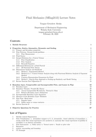
  • 24. 3.4 Measures of the Boundary Layer Thickness The neighborhood of the interfaces, where the fluid variables evolve from the interface to the free-stream values denoted by the BL thickness, or alternatively linked to other different physical phenomena. The following equation summarizes boundary layer variables, conditions in relation to free stream values BL Vel. . u(x, y = δ(x)) = Ue(x) Defined δ BL Temp. . T(x, y = δT (x)) = Te(x) Defined δT BL Concent./Mass . CA(x, y = δC(x)) = CAe(x) Defined δC BL Vel. . u(x, y = δ99(x)) = 0.99Ue(x) BL Approx. 99% free stream BL Temp. . T(x, y = δ99(x)) − T0 = 0.99(Te − T0) Approx. BL 99% Free stream BL Concent. . CA(x, y = δ99(x)) − CA0 = 0.99(CAe − CA0) Approx. Mass BL 99% Free stream (29) Example15: A researcher is interested in the aerodynamic resistance FD of spheres. He conducts several experiments in an aerodynamic tunnel at atmospheric conditions ρ = 1.2 kg m3 and µ = 1.8 × 10⁻⁵ kg ms with a sphere of a diameter D = 10cm, concluding that FD = 0.0015V 1 .92 where V is the uniform upstream air velocity. a. Determine the correlation between CD = FD 1 2 ρV 2D2 and Re = ρV D µ with potential correlation CD = KRem by determining m. b. Determine the resistance of a D = 2cm sphere at an air speed of V = 1m/s. Solution a Expanding the dimensionless equation, CD = KRem FD 1 2 ρV 2D2 = C( ρV D µ )m F = C 1 2 ρV 2 D2 ( ρV D µ )m Maintaining consistency with the empirical relation taking out V, FD = 0.0015V 1 .92 = C 1 2 ρD2 ( ρD µ )m V (2+m) Collecting like terms, 0.0015 = C 1 2 ρD2 (ρD µ )m and 2+m = 1.92 that the later one gives m = −0.08 while substituting the value yields C = 0.0015 (1 2 1.2kg/m3 × (10cm)2( 1.2kg/m310cm 1.8x10⁻⁵kg/ms )−0.08 C = 0.306 b Therefore, the correlation is CD = 0.306Re−0.08 and if sphere diameter is 2cm, and air speed 1m/s, Re = ρV D µ = 1.2×1m/s×2cm 1.8×10−5 = 1333 and CD = 0.306Re−0.08 = 0.2846 with FD = 1 2 CDρ(V D)2 = 6.83 × 10⁻⁵ N 3.5 Pipe Flow: Head losses This section involves an important practical fluids engineering problem: flow in ducts with various velocities, various fluids, and various duct shapes. Piping systems are encountered in almost every engineering design and thus have been studied extensively. There is a small amount of theory plus a large amount of experimentation. The head losses for a steady incompressible flow in a constant section pipe could be expressed by the Darcy Weisbach equation hf = ∆P ρg = λ( ϵ D , ReD) L D u2 2g (30) Where D is pipe diameter, L the pipe length U the mean velocity and the ϵ characteristic length of the roughness. The equation can also be determined by dimensional analysis and similitude Exercise 3 Drive the expression in Equation 30 with the help of dimensional analysis. Correlations for the friction factor in circular cross-section pipes as presented in the table below. Some correlations for λ. Also, the Moody Diagram 15 depicts graphically the friction Table 7: Pipe Friction Factor for Different Flow Regime Flow Regime . Friction Factor λ Laminar ReD¡2300 64 ReD Turbulent ReD 2300 1 √ λ Colebrook = −2.0log(ϵ/D 3.7 + ReD √ λ ) Fully rough ReD √ λ ϵ/D 70 1 √ λ Nikuradse = −2.0log(ϵ/D 3.7 ) smooth Pipes 1 √ λ Prandtl = −2.0log(ReD √ λ) − 0.8 factor as a function of the Reynolds number based on the pipe diameter and the relative roughness as shown in the figure below 22
  • 25. Figure 14: horizontal pipe flow regions 3.5.1 Singular losses Besides constant section straight pipes, one can find components such as bends, valves, Tees, expansions and so on. In these elements, the viscous dissipation gives rise to energy losses, which are called singular or local head losses from Moody diagram based on The Reynolds number is based on the pipe diameter D. The pressure loss given by the Darcy-Weisbach equation and τ0 as a function of friction coefficient cf λ L D 1 2 ρU2 πD2 4 = Cf 1 2 ρU2 π where Cf = λ 4 (31) The where Ks is the dimensionless singular head loss coefficient. The constant Ks depends on the element type and its geometry given in 8. Therefore, for each new design,it has to be experimentally determined. Typically, for high Reynolds numbers,Ks is considered independent of Re and so, can be taken as a constant. The reference velocity U can be the upstream or downstream mean velocity. The basic momentum correlations coefficient of Table 8 are for constant property boundary layers. Example 16: As you could see from 8, the accepted transition Reynolds number for flow in a circular pipe is Table 8: Singular loss coefficient and Basic momentum correlation coeffcient for various flow regime [4] Geometry Regime Correlation Ks flat plate Laminar Rex 3 × 10⁵ Cfx = 0.664Rex −1/2 Laminar Rex 3 × 10⁵ CfL = 1.328ReL −1/2 Turbulent Rex 3 × 10⁵ Cfx = 0.664Rex −1/5 Pipe Laminar ReD 2300 Cf = 16 ReD Turbulent 3 × 10⁴ ReD 106 Cf = 0.046Re −1/5 D Elements Ks Outlet off tank into pipe 0.05-1 Sudden expansion (1 − A1 A2 )2 Sudden Contraction 0.42(1 − A1 A2 ) if D2/D1 ≤ 0.76 (1 − A1 A2 )2 if D2/D1 ≤ 0.76 Long Radius 90o Elbow 0.4 Long Radius 90o Elbow 0.9 Valve Fully Open 0.03-14 Get Valve Fully Open 0.1 Globe Valve Fully Open 8.0 Red, crit = 2300. For flow through a 5cm diameter pipe, at what velocity will this occur at 20o C for (a) airflow and (b) water flow? Solution Almost all pipe flow formulas are based on the average velocity V = Q/A, not centerline or any other point velocity. Therefore, the transition is specified at ρV D µ = 300. With D known, we introduce the appropriate fluid properties at 20o C from Standard Table as shown below: Table 9: Common Fluid Properties at 20oC [1] Common Fluids properties/parameters 23
  • 26. Figure 15: Moody Diagram [9][10] 24
  • 27. Liquid ρ, kg/m3 µ, kg/(m · s) Y, N/m∗ pv, N/m2 Bulk modulus, N2 Viscosity parameter C∗ Ammonia 608 2.20 × 10⁻⁴ 2.13 × 10⁻² 9.10 × 10+ 5 − 1.05 Benzene 881 6.51 × 10⁻⁴ 2.88 × 10⁻² 1.01 × 10⁴ 1.4 × 10⁹ 4.34 Carbon tetrachloride 1, 590 9.67 × 10⁻⁴ 2.70 × 10⁻² 1.20 × 10⁴ 9.65 × 10⁸ 4.45 Ethanol 789 1.20 × 10⁻³ 2.28 × 10⁻² 5.7 × 10³ 9.0 × 10⁸ 5.72 Ethylene glycol 1, 117 2.14 × 10⁻² 4.84 × 10⁻² 1.2 × 101 − 11.7 Freon 12 1, 327 2.62 × 10⁻⁴ − − − 1.76 Gasoline 680 2.92 × 10⁻⁴ 2.16 × 10⁻² 5.51 × 10⁴ 9.58 × 10⁸ 3.68 Glycerin 1, 260 1.49 6.33 × 10− 2 1.4 × 10⁻² 4.34 × 10⁹ 28.0 Kerosine 804 1.92 × 10⁻³ 2.8 × 10− 2 3.11 × 10³ 1.6 × 10⁹ 5.56 Mercury 13, 550 1.56 × 10− 3 4.84 × 10⁻¹ 1.1 × 10⁻³ 2.55 × 101 0 1.07 Methanol 791 5.98 × 10⁻⁴ 2.25 × 10− 2 1.34 × 10⁴ 8.3 × 10⁸ 4.63 SAE oil 10W30 870 1.04 × 10− 1∗ 3.6 × 10−2 − 1.31 × 10⁹ 15.7 SAE oil 876 1.7 × 10⁻¹ ∗ − − − 14.0 SAE 30W oil 891 2.9 × 10−1 ∗ 3.5 × 10−2 − 1.38 × 10⁹ 18.3 SAE 50W oil 902 8.6 × 10⁻¹ ∗ − − − 20.2 Water 998 1.00 × 10− 3 7.28 × 10⁻² 2.34 × 10³ 2.19 × 10⁹ Table A.1 Seawater (30%) 1, 025 1.07 × 10− 3 7.28 × 10− 2 2.34 × 10+ 3 2.33 × 10+ 9 7.28 Selecting relevant properties from 9, (a) Air: ρV d µ = (1.205 kg/m3 )V (0.05 m) 1.80×10⁻⁵ kg/(m·s) = 2300 or V ≈ 0.7m s (b) Water: ρV d µ = (998 kg/m3 )V (0.05 m) 0.001 kg/(m·s) = 2300 or V = 0.046m s Example 17: Work Moody’s problem in Figure 15 backward to find the unknown 6in diameter if the flow rate Q = 1.18ft3 /s is known. Recall L = 200ft, ϵ = 0.0004ft, and ν = 1.1 × 10− 5ft2 /s. Solution Write f, Red, and ϵ/d in terms of the diameter: f = π2 8 ghf d5 LQ2 = π2 8 32.2ft/s2 (4.5ft)d5 (200ft) (1.18ft3/s) 2 = 0.642d5 or d ≈ 1.093f1/5 Red = 4 1.18ft3 /s π (1.1 × 10r − 5ft2/s) d = 136, 600 d ϵ d = 0.0004ft d with everything in BG units, of course. Guess f; compute d , Red , and ϵ/d ; and then compute a better f from the Moody chart. Repeat until convergence. With an an initial f ≈ 0.03 guess: f ≈ 0.03 d ≈ 1.093(0.03)1/5 ≈ 0.542ft Red = 136, 600 0.542 ≈ 252, 000 ϵ d ≈ 7.38 × 10⁻⁴ fnew ≈ 0.0196 dnew ≈ 0.498ft Red ≈ 274, 000 ϵ d ≈ 8.03 × 10⁻⁴ fbetter ≈ 0.0198 d ≈ 0.499ft Convergence is rapid, and the predicted diameter is correct, about 6 in. The slight discrepancy (0.499 rather than 0.500ft) arises because hf was rounded to 4.5ft. Example 18 Consider to measure the volume flow of water ρ = 1000kg3 /m3 , ν = 1.02 × 10⁻⁶ m2 /s moving through a 200mm diameter pipe at an average velocity of 2.0m/s. If the differential pressure gage selected reads accurately at p1 − p2 = 50, 000Pa, what size meter should be selected for installing (a) an orifice with D : 1 2 D taps, (b) a long-radius flow nozzle, or (c) a venturi nozzle? What would be the nonrecoverable head loss for each design? Solution Here the unknown is the β ratio of the meter. Since the discharge coefficient is a complicated function of β, iteration will be necessary. We are given D = 0.2m and V1 = 2.0m/s. The pipeapproach Reynolds number is thus ReD = V1D y = (2.0)(0.2) 1.02 × 10−6 = 392, 000 For all three cases [(a) to (c)] the generalized formula 3.5 holds: Vt = V1 β2 = α 2 (p1 − p2) ρ 1/2 α = Cd (1 − β4) 1/2 25
  • 28. where the given data are V1 = 2.0m/s, ρ = 1000kg/m3 , and ∆p = 50, 000Pa. Inserting these known values into above Eq. gives a relation between β and α : 2.0 β2 = α 2(50, 000) 1000 1/2 or β2 = 0.2 α The unknowns are β (or α ) and Cd. Parts (a) to (c) depend upon the particular chart or formula needed for Cd = f (ReD, β). We can make an initial guess β = 0.5 and iterate to convergence. Part (a) For the orifice with D : 1 2 D taps, use Eq the given above and Table 30. The iterative sequence is β1 = 0.5, Cd1 = 0.604, α1 = 0.624, β2 = 0.566, Cd2 ∼ 0.606, α2m0.640, β3 = 0.559 We have converged to three figures. The proper orifice diameter is d = βD = 112mm Ans. (a) Part (b) For the long radius flow nozzle, Fig.15 or iteration. The iterative sequence is β1 ≈ 0.5, Cd1 ≈ 0.9891, α1 = 1.022, β2 ≈ 0.442, Cd2 = 0.9896, α2n1.009, β3 = 0.445 We have converged to three figures. The proper nozzle diameter is d = βD = 89mm Part (c) For the venturi nozzle, use or . The iterative sequence is β1 ≈ 0.5, Cd1 ≈ 0.977, α1 ≈ 1.009, β2 = 0.445, Cd2 ≈ 0.9807, α2 = 1.0004, β3 = 0.447 We have converged to three figures. The proper venturi diameter is d = βD = 89mm Ans. (c) 3.5.2 Orifice meter or venna contracta As demonstrated in figure 3, the solution can be attained alternatively, the velocity of the fluid flow on the vena contracta is defined according to [2] by V2 = 1 r 1 − D2 D1 4 p 2g∆h and the actual flow rate is determined by Qact = cOAO r 1 − DO D1 4 p 2g∆h where: Qact = actual flow rate CO = coefficient of discharge for orifice AO = cross section area of the orifice D1 = pipe diameter, (29mm) Do = orifice diameter, (20mm) ∆h = difference in pressure head subsubsectionVenturimeter The venturi meter also exploits pressure difference between flow at inlet and flow at throat by applying the Bernoulli’s equation. The equation In this equipment, the flow rate is defined by Qact = cV A2 r 1 − D2 D1 4 p 2g∆h where: Qact = actual flow rate CV = coefficient of discharge for venturi A2 = cross section area of the throat D1 = pipe diameter, (29mm) D2 = throat diameter, (17mm) ∆h = difference in pressure head subsubsectionPitot tube and Rotameter Pitot Tube is a kind of flow meter instrument that applies the pressure difference of the stagnation point and another place on fluid flow. In this case, the velocitiy of fluid flow on the stagnation point is assumed as zero. The equation to calculate the actual flow rate of flowing liquid is Qact = CP A1 p 2g∆h where : Qact = actual flow rate CP = coefficient of discharge for pitot tube A1 = cross section area of the pipe (D1=19 mm) ∆h = difference in pressure head Rotameter This kind of flowing instrument is applying the force balance on the floater for measuring the flow rate. The equation for determining the velocity of the fluid is where : Vf = velocity of the fluid flow Vfloater = volume of the floater CD = coefficient of the discharge Afloater = Cross section area of the floater g = 9.81m/s2 For solved problems on flow measurement, please visit the website [11] 26
  • 29. 3.6 Review Exercise B 1. Verify the order of magnitude of δ, δT , δC for laminar flow. 2. Drive the the expressions derived for the relative boundary layer thicknesses at Section 26 3. Are low-speed, small-scale air and water boundary layers really thin? Consider flow at U1 = ft/s past a flat plate 1ft long. Compute the boundary layer thickness at the trailing edge for (a) air and (b) water at 20o C. 4 Objective Questions for Practice Practice questions with free feedback can be accessed online via [12], more questions at [13], further at [14] and [15] 1. Free surface of a liquid tends to contract to the smallest possible area due to force of (a) Surface tension (b) Viscosity (c) Friction (d) Cohesion 2. The Metacentric heights of two floating bodies A and B are 1m and 1.5m respectively. Select the correct statement. (a) The bodies A and B have equal stability (b) The body A is more stable than body B (c) The body B is more stable than body A (d) The bodies A and B are unstable 3. The rise or depression of liquid in a tube due to surface tension will increase in size of tube will (a) Increase (b) Remain unaffected (c) May increase or decrease depending on the characteristics of liquid 4. A body floats in stable equilibrium (a) When its meatcentric height is zero (b) When the metacentre is above e.g. (c) When its e.g. is below its center of buoyancy (d) Metacentre has nothing to do with position of e.g. for determining stability 5. The total pressure on a horizontally immersed surface is (where w = Specific weight of the liquid, A = Area of the immersed surface, and x = Depth of the centre of gravity of the immersed surface from the liquid surface) (a) wA (b) wx (c) wAx (d) wA/x 6. The discharge of a depressed nappe is 6 to 7 percent that of a free nappe. (a) Less than (b) More than (c) Equal to (d) None of these 7. The line of action of the buoyant force acts through the Centroid of the (a) Submerged body (b) Volume of the floating body (c) Volume of the fluid vertically above the body 27
  • 30. (d) Displaced volume of the fluid 8. The intensity of pressure at any point, in a liquid, is (a) Directly proportional to the area of the vessel containing liquid (b) Directly proportional to the depth of liquid from the surface (c) Directly proportional to the length of the vessel containing liquid (d) Inversely proportional to the depth of liquid from the surface 9. During the opening of a valve in a pipe line, the flow is (a) Steady (b) Unsteady (c) Uniform (d) Laminar 10. A manometer is used to measure (a) pressure (b) temperature (c) flow rate (d) density 11. For hypersonic flow, the Mach number is (a) Unity (b) Ma 1 (c) Ma 1 (d) Ma 2 12. The theoretical velocity of jet at vena contracta is (where H = Head of water at vena contracta) (a) 2gH (b) H × √ (2g) (c) 2g × √ H (d) √ (2gh) 13. For pipes, laminar flow occurs when Reynolds number is (a) Less than 2000 (b) Between 2000 and 4000 (c) More than 4000 (d) Less than 4000 14. When the flow in an open channel is gradually varied, the flow is said to be (a) Steady uniform flow (b) Steady non-uniform flow (c) Unsteady uniform flow (d) Unsteady non-uniform flow 15. Property of a fluid by which molecules of different kinds of fluids are attracted to each other is called (a) Adhesion (b) Cohesion (c) Viscosity (d) Compressibility 16. What is fluid mechanics? (a) Study of fluid behaviour at rest 28
  • 31. (b) Study of fluid behaviour in motion (c) Study of fluid behaviour at rest and in motion (d) Study of fluid behaviour at rest and in motion 17. Which of the following is the basic principle of fluid mechanics? (a) Momentum principle (b) Energy equation (c) Continuity equation (d) All of the mentioned 18. What is fluid mechanics used for? (a) Fluid mechanics enables to comprehend the behaviour of solid fluids under pressure (b) Fluid mechanics enables to comprehend the behaviour of fluids under a variety of forces atmospheric conditions (c) Fluid mechanics enables to comprehend the behaviour of fluids under various temperatures only (d) None of the mentioned 19. Stagnation point is the point in fluid mechanics where the velocity of the fluid at that point is (a) unity (b) constant (c) infinite (d) zero 20. Eddy viscosity is a turbulent transfer of (a) Fluid (b) Heat (c) Momentum (d) Pressure 21. Which among the following is the equation for Bernoulli? (a) Tds = dh − vdp (b) Tds = dh (c) Tds = dh + vdp (d) Tds = dh/vdp 22. For an isentropic flow (a) Enthalpy = 0 (b) Entropy = 0 (c) Pressure = 0 (d) Temperature = 0 23. Which one of the following is a major loss? (a) frictional loss (b) shock loss (c) entry loss (d) exit loss 24. Which property of the fluid accounts for the major losses in pipes? (a) density (b) specific gravity (c) viscosity (d) compressibility 29
  • 32. References [1] Y. Cengel, J. Cimbala, Fluid mechanics fundamentsls and applications (in si units), Tata McGraw Hill, 2006. [2] T. H. Williamson, A. Harris, The British Journal of Ophthalmology 1994, 78, 939. [3] R. De Leeuw, Liquid correction of Venturi meter readings in wet gas flow, 1997. [4] G. Hauke, R Moreau, An introduction to fluid mechanics and transport phenomena, Vol. 86, Springer, 2008. [5] B. R. Munson, T. H. Okiishi, W. W. Huebsch, A. P. Rothmayer, Fluid mechanics, Wiley Singapore, 2013. [6] H. Lomax, T. H. Pulliam, D. W. Zingg, T. Kowalewski, Appl. Mech. Rev. 2002, 55, B61–B61. [7] G. I. Barenblatt, B. G. Isaakovich, Scaling, self-similarity, and intermediate asymptotics: dimensional analysis and intermediate asymptotics, Cambridge University Press, 1996. [8] J. Schumacher, EPL (Europhysics Letters) 2007, 80, 54001. [9] E. F. Adiutori, Open Mechanical Engineering Journal 2009, 3, 43–48. [10] J. M. C. yunus A. Cengel, Fluid Mechanics: Fundamentals and Applications, 2006. [11] M. Selamat, M. Rahim, International Journal of Information Management 1996, 16, 299–313. [12] Fluid Mechanics Multiple Choice Questions and Answers, https : / / www . objectivebooks . com / fluid - mechanics-multiple-choice/, MCQ Fluid Mechanics, Accessed January 25, 2025. [13] Fluid Mechanics MCQ Questions, https : / / testbook . com / objective - questions / mcq - on - fluid - mechanics -- 5eea6a0c39140f30f369e136/, Objectivebooks MCQ Fluid Mechanics, Accessed January 25, 2025, 2023. [14] M. Bhojasia, Fluid Mechanics Multiple Choice Questions and Answers, https://www.sanfoundry.com/1000- fluid-mechanics-questions-answers/, sanfoundry Fluid Mechanics, Accessed January 25, 2025. [15] Fluid Mechanics Interview Questions and Answers, https://engineeringinterviewquestions.com/fluid- mechanics-interview-questions-and-answers//, sanfoundry Fluid Mechanics, Accessed January 25, 2025. 30