
Empfohlen
Weitere ähnliche Inhalte
Was ist angesagt?
Was ist angesagt? (20)
Ähnlich wie Introduction to Deep Reinforcement Learning
Ähnlich wie Introduction to Deep Reinforcement Learning (20)
Mehr von IDEAS - Int'l Data Engineering and Science Association
Mehr von IDEAS - Int'l Data Engineering and Science Association (20)
Kürzlich hochgeladen
Kürzlich hochgeladen (20)
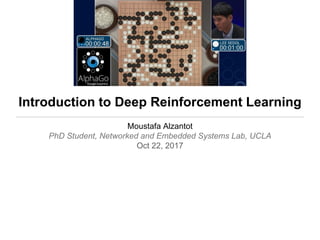
Introduction to Deep Reinforcement Learning
- 1. Introduction to Deep Reinforcement Learning Moustafa Alzantot PhD Student, Networked and Embedded Systems Lab, UCLA Oct 22, 2017
- 2. Machine Learning Computer programs can increase their performance on a given task without being explicitly programmed for it, just by analyzing data !
- 3. Types Machine Learning • Supervised Learning • Given a set of labeled examples , predict the output label for new unseen inputs. • Unsupervised Learning • Given unlabeled dataset, understand the structure of the data (e.g. clustering, dimensionality reduction). • Reinforcement Learning • Branch of machine learning concerned with acting optimally in face of uncertainty (i.e. learning to do ! )
- 4. Reinforcement Learning • Agent observes the environment state, performs some action. • In response, the environment state changes and agent receives reward. • Goal of agent is to pick actions that maximizes the total reward received from environment. Environment Agent Actions: a State: s Reward: r Source: Pieter Abeel, UC Berkley188
- 5. Examples
- 6. Ex: Grid World A maze-like problem The agent lives in a grid Walls block the agent’s path Noisy movement: actions do not always go as planned 80% of the time, the action North takes the agent North (if there is no wall there) 10% of the time, North takes the agent West; 10% East If there is a wall in the direction the agent would have been taken, the agent stays put The agent receives rewards each time step Small “living” reward each step (can be negative) Big rewards come at the end (good or bad) Goal: maximize sum of rewards Source: Pieter Abeel, UC Berkley188
- 7. Ex: Grid World Deterministic Grid World Stochastic Grid World
- 8. Markov Decision Process • MDP is used to describe RL environments. • MDP is defined by: • A set of states s S A set of actions a A A transition function Probability that a from s leads to s’, i.e., P(s’| s, a) Also called the model or the dynamics A reward function Sometimes just R(s) or R(s’) Discount factor Environment Agent Actions: a State: s Reward: r Source: Pieter Abeel, UC Berkley188
- 9. Discounting It’s reasonable to maximize the sum of rewards It’s also reasonable to prefer rewards now to rewards later One solution: values of rewards decay exponentially 0 < < 1 Worth Now Worth Next Step Worth In Two Steps Why discount ? — sooner rewards will probably have higher utility than later rewards — Control preferences of different solutions. — Avoid numerical issues (total rewards going to infinity)
- 10. Optimal policy No penalty at each step • Reward for each step: -0.1 • Reward for each step: -2 • Reward for each step: +0.1
- 11. Remember MDPs • MDP is defined by: • A set of states s S A set of actions a A A transition function Probability that a from s leads to s’, i.e., P(s’| s, a) Also called the model or the dynamics A reward function Sometimes just R(s) or R(s’) Discount factor Environment Agent Actions: a State: s Reward: r
- 12. Solving MDPs • If the MDP (environment model) is known, there are ways that are guaranteed to find the optimal policy.
- 13. Value-function The value (utility) of a state s: V*(s) = expected utility starting in s and acting optimally The value (utility) of a q-state (s,a): Q*(s,a) = expected utility starting out having taken action a from state s and (thereafter) acting optimally The optimal policy: *(s) = optimal action from state s
- 14. GridWorld: Q-Values Noise = 0.2 Discount = 0.9 Living reward = 0 Source: Pieter Abeel, UC Berkley188
- 15. Value Iteration Theorem: will converge to unique optimal values Basic idea: approximations get refined towards optimal values Policy may converge long before values do • Alpaydin: Introduction to Machine Learning, 3rd edition
- 16. Policy Iteration • Value-iterations iterates to refine the value function estimates until it converges. • Optimal policy often converges before the value function. • The final goal is to get an optimal policy. • Policy-iteration: iterates to re-define the policy at each step. • Alpaydin: Introduction to Machine Learning, 3rd edition
- 18. Model-Based Learning Model-Based Idea: Learn an approximate model based on experiences Solve for values as if the learned model were correct Step 1: Learn empirical MDP model Count outcomes s’ for each s, a Normalize to give an estimate of Discover each when we experience (s, a, s’) Step 2: Solve the learned MDP For example, use value iteration, as before
- 19. Model-Free Learning • Directly learn the V and Q value functions without estimating T and R. • Remember: Key question: how can we do this update to V without knowing T and R? In other words, how to we take a weighted average without knowing the weights?
- 20. Q-Learning Use Temporal difference to learn Q(s, a) from observed samples. After convergence, extract the optimal policy !
- 21. How to Explore? Several schemes for forcing exploration Simplest: random actions (-greedy) Every time step, flip a coin With (small) probability , act randomly With (large) probability 1-, act on current policy Problems with random actions? You do eventually explore the space, but keep thrashing around once learning is done One solution: lower over time Another solution: exploration functions
- 22. Demo: MountainCar using Q-Learning https://www.youtube.com/watch?v=ByOdncJE5bE
- 24. Approximate Q Learning Basic Q-Learning keeps a table of all q-values In realistic situations, we cannot possibly learn about every single state! Too many states to visit them all in training Too many states to hold the q-tables in memory
- 25. Approximate Q-Learning Using a feature representation, we can write a q function (or value function) for any state using a few weights: Use optimization to find the weights that minimize MSE between predicted and observed Q-values. Questions: How to approximate the Q(s, a) function ? How to compute these features ?
- 26. Deep Q Networks Remember: Universal approximation theorem: Neural Network with 1 hidden layer can learn any bounded continuous function!
- 27. Deep Q Networks Remember: Deep neural networks are good as feature extractors !
- 28. Deep Q Networks
- 31. Deep Q-Network training Experience Replay Trick
- 32. DQN Results in Atari
- 33. Resources • Pieter Abeel, UC Berkley CS 188 • Alpaydin: Introduction to Machine Learning, 3rd edition • David Silver, UCL Reinforcement Learning Course • Yandex: Practical RL • MIT: Deep Learning for self-driving cars ! • Stanford 234: Reinforcement Learning
- 34. Thanks Send any question to malzantot@ucla.edu