2. Introduction
Aeromagnetic survey maps the variation in geomagnetic field, which occurs due to the changes in the percentage of magnetite in rock. It
reflects the variation in the distribution and type of magnetic minerals in the subsurface. Magnetic minerals can be mapped from the surface to
greater depth in crustal rocks depending on dimension, shape, and the magnetic property of the rock. Sedimentary formations do not usually
have appreciable magnetic properties, this is because of the minute contribution of detrital remnant magnetism while igneous and metamorphic
rocks exhibit greater variations and become useful in exploring bedrock geology.
Ado-Ekiti Southwest and its adjoining areas has witnessed several geophysical investigations such as VLF (very low frequency) and VES
(vertical electrical sounding) studies, borehole logging (lithologic and geophysical), electrical resistivity probing, electromagnetic surveys,
surface mapping among others to determine its groundwater potential and evaluate its geologic and economic values but little has been done in
the area of magnetic mineral prospecting or exploration. Therefore, the need for a cost effective, rapid result, risk reduction and faster
technique like aeromagnetic method which can give quick and reliable information about the subsurface basement structures, subsurface
lithology, trend, depth to magnetic source, and structural features of large and inaccessible areas is necessary hence, this study.
The study area is located within the basement complex region of Nigeria and indicators that have been found useful in mineral exploration
includes faults, fractures (lineaments), arched, or domed structures in addition to oxidized and hydrothermally altered areas (Peterson et al.,
1976), and the application of aeromagnetic methods amplifies the recognition of the difference in depths of magnetic sources, structures like
faults, dike, lineaments, and layered magnetic susceptibility given in the variability of complexes. This report is supposed to serve as a guide
for geologically related decision making prior to exploration and constructions. The study area is located between longitudes 5°00´ E and 5°15´
E and latitudes 7°30´ N and 7°45´ N, covering an area of 1,471.5 km2.
Geological Setting
The study area is part of the basement complex of southwestern Nigeria and is Archean to early Proterozoic in age as described by Talabi
(2013). More so, Oversby (1975) and Olanrewaju (1981) indicated that the study area is composed of migmatite-gneiss-quartzite complex with
little supra-crustal rock relics. The basement complex of Nigeria is zoned in the western part of the Pan-African shield as described by
McMurry (1976) and Ball (1980), occurring in the mobile zone of the Pan-African reactivation area between the West-African craton to the
west and the Congo craton to the southeast.
The following distinguishable lithologies can be identified from the geologic map of the study area (Figure 1) and they are; quartzite,
migmatite, schist with pegmatite intrusion, biotite rich granites, charnokitic rocks, and quartz veins.
3. Aeromagnetic Data and Analysis
Data Acquisition
As part of a nationwide high resolution airborne geophysical survey aimed at assisting and promoting mineral exploration in Nigeria,
aeromagnetic data was acquired between 2003 and 2009 by Fugro Airborne Survey Limited for the Nigerian Geological Survey Agency
(NGSA) (MMSD, 2010). The data was collected systematically by dividing the country into geological blocks with dissimilar measurement
parameters for each block with the eventual production of an aeromagnetic map for the whole country.
The Scintrex CS3 Cesium Vapor magnetometer was used and it is an optically pumped cesium vapor magnetometer used for scalar
measurement of the Earth’s magnetic field. It can be used in a variety of applications such as airborne, satellite, ground magnetometry, or
gradiometry. It is highly sensitive and measures in the range of pT (1 pT = 0.001 nT) in a measuring bandwidth of 1 Hz and this sensitivity
does not deteriorate as the measured ambient field decreases. It measures between 15,000 nT and 100,000 nT. The sensor head has an
electrode-less discharge lamp (containing cesium vapor) and absorption cell. Electrical heaters bring the lamp and the cell to optimum
operating temperatures with control and driving circuits located in the electronics console. Heating currents are supplied to the sensor head
through the interconnecting cable.
The area under study, Ado-Ekiti Southwest and its environs designated as Sheet 244; is part of Block B and was surveyed in Phase 1 of the
project. The survey was carried out by fixed wing (Cessna) aircraft covering a total of 235,000 line kilometers with a flight spacing of 200
meters and a terrain clearance of 80 meters, The flight direction was NW-SE with tie-line spacing of 200 meters and tie-line direction of NE-
SW.
A recording interval of 0.1 secs and a grid mesh size of 50 meters were applied in the World Geodetic System of 1984 (WGS84) within UTM
Zone 36S and with the Clark 1880/Arc 1960 coordinate system.
Data Processing
The data is that of total field and is in a gridded form as a total magnetic intensity (TMI) map (see Figure 2). This method fits minimum
curvature curves (which is the smoothest possible surface that would fit the given data values) to data point using method described by Briggs
(1974).
Data Filtering
Butterworth filter which is a low-pass filter was applied in accordance with I.G.R.F reduction technique. A low-pass filter is a filter that passes
low-frequency signals and attenuates (reduces the amplitude of) signals with frequencies higher than the cut off frequency. The actual amount
of attenuation for each frequency varies depending on specific filter design. Low-pass Butterworth filter was applied to the total magnetic
intensity data to remove regional effects. An ideal low-pass filter completely eliminates all frequencies above the cut off frequency while
4. passing those below unchanged. The residual magnetic intensity (RMI) data were processed using Butterworth low pass filtering technique to
increase the signal to noise ratio and to remove all high frequency events which are representative of cultural, processing, or other forms of
noise or error in the data and then subjected to further processing.
Downward continuation, a low cut and optimum filter were also applied to enhance responses emanating from shallower sources; this was
achieved by moving the detector closer to the source. The principle is such that, short wavelength signals are likely to originate from shallow
sources, hence signals originating from a particular depth source could be selected based on wavelength. A plot of radially averaged power
spectrum was used to determine the wavenumbers corresponding to shallower sources; consequently, everything below the wavenumber
corresponding to the depth of interest was treated as noise and silenced using low cut filter in line with (Osinowo and Olayinka, 2013).
Upward continuation filtering were subsequently applied to filtered data and transforms the data into that which would have been measured at a
higher altitude than at which it was actually measured. It is useful for smoothing data, among other things. Since, this filter is considered a
‘clean’ filter because it produces no side effect that may require the application of other filter or process to correct. In this case, it is often used
to remove or minimize the effects of shallow sources and noise in grids.
Reduction to Magnetic Equator
To produce anomalies depends on the inclination and declination of the body’s magnetization, inclination, and declination of the local earth’s
field and orientation of the body with respect to the magnetic north (Baranov, 1957), it is usually necessary to perform a standard phase shift
operation known as Reduction-to-Pole (RTP) on the observed magnetic field. In magnetic equatorial regions where inclination is less than 15°,
RTP is generally unstable and cannot be derived because such data introduces north – south alignment of the anomalies into the data, thereby
making the data unstable. A similar effect is seen when a magnetic field is Reduced-to-Equator (RTE) instead of to the pole depending on the
latitudinal position of the study area. Once the field has been reduced to the equator, the regional magnetic field will be horizontal and most of
the source magnetizations will be horizontal.
For the vital purpose of accurate positioning, the total magnetic intensity map was reduced to equator prior further processing to correct for
effect of latitude and to make the magnetic anomalies to be symmetrically centered over their corresponding sources because the study area is
closer to the equator. In this report, RTE was applied to the filtered map with -10.7240
and -4.8800
representing the inclination and declination
respectively of the geomagnetic field parameters of the central location of the study area as seen in Figure 3 and was used for the reduction.
The airborne magnetic datasets were further processed with respect to Figure 4.
Method
With the main aim of analysing, detecting, and interpreting the available aeromagnetic map of the study area to identify the possible tectonic
setting as well as subsurface structures, Mineralized zones and propose a new geological map of the area under study, the approach used by
Feumoe et al., (2012) was adopted. This method includes the use of the FVD method to detect linear structures, the pseudo-gravity to delineate
5. crustal magnetic sources while the Euler deconvolution and the average power spectrum are used to determine depths of deep and shallow
magnetic body sources.
First Vertical Derivatives (FVD)
Derivative filtering techniques are used to sharpen the edges of magnetic anomalies and better locate their positions. The reduced to the equator
total magnetic intensity map contains all the anomalies representative of both shallow and deep sources. Therefore, derivative filtering
techniques are to be applied on it so as to suppress unwanted sources (and enhance some) or to sharpen the edges of the anomalies. Vertical
derivatives enhancement sharpens up anomalies over bodies and tends to reduce anomaly complexity and allow clearer imaging of the
causative structures. Vertical derivatives map/profile enhance the lineament and anomalies owing to their short wavelength character.
When the first vertical derivatives is applied on the magnetic data, it enhances shallow wavelength features, that are results of near surface
structures, and suppresses long wavelength ones (deeper sources) thereby provide a better and clearer picture of the subsurface.
The first vertical derivatives filter was applied to the reduced to equator, total magnetic intensity data to enhance local anomalies obscured by
the broader regional trend. In this case, it amplifies short wavelength components of the field and de-emphasizing the long wavelength
components thereby giving clearer contrast between the geologic units.
The tilt derivative in Figure 5a and Figure 5b, amplifies lineaments, which are structural deformations that are related to faults, joints, and
arched zones or even geological contacts. Magnetic minerals are mainly concentrated along or aligned with some structures or sedimentary
features such as faults or channels. The tilt map (Figure 5) has the parallel and sub parallel lineaments picked out.
Pseudo-gravity
According to Pratt and Shi (2004), the pseudo-gravity transformation is one of many possible FFT techniques that can be applied to
aeromagnetic data. It enhances the anomalies associated with deep magnetic sources at the expense of the dominating shallow magnetic
sources. This transformation is an excellent interpretation tool for the detection of deep, magnetic igneous plutons and volcanic piles and the
transformed data can be modelled using conventional gravity modelling tools. It is a suitable tool for interpreting deep-seated mineral plumbing
systems associated with known, shallow mineral occurrences.
The enhanced pseudo-gravity transform is derived from the standard pseudo-gravity transform by removing long wavelength anomalies that are
associated with FFT processing properties and deep crustal magnetic sources. Conventional low-pass and upward continuation filters were
considered but a modelling approach was adopted to remove the influence of magnetic sources that are beyond the zone of exploration interest.
The pseudo-gravity data can be modelled using conventional map modelling and inversion methods, where the density is considered as a
pseudo-density defined by the relationship
6. D = kH/γ, 1
Where D is the density contrast, k is magnetic susceptibility, H is the total magnetic field intensity, and γ is the universal gravitational constant.
This relationship assumes that the magnetization is induced and no remanence is present.
Power Spectrum and Euler Deconvolution
Each wavelength’s power unit can be plotted against wavenumber regardless of direction, to produce a power spectrum. In frequency domain,
one can prepare and analyse the distribution of short to long wavelength across all measured high to low frequency. The power spectrum can be
broken into series of straight lines segments and each segment represents the cumulative response of a discrete assemblage of sources at a
given depth. The depth is directly proportional to the slope of the line segment (Spector and Grant, 1970). Potential field may be considered as
representing a series of interfering waves of different wavelengths and directions.
The slope of each segment provides information about the depth to the bottom of the magnetic bodies (Kivior and Boyd, 1998). Radially
averaged power spectrum of magnetic data according to Blanco-Montenego et al., (2003) is expressed as a function of wavenumber and is
related to depth to the bottom of the deepest sources as expressed in equation 2.
Kmax 2
Where Zt and Zb are depth to top and depth to bottom of the magnetic sources respectively. K is a function of wavenumber which is expressed
in radian per unit distance.
In this study, power spectrum analysis was carried out on aeromagnetic data using Geosoft® Oasis Montaj™ software to identify average
depths of source assemblage. This same technique was also adopted to attempt identification of the characteristic depth of the magnetic
basement, on a moving window basis, merely by selecting the steepest and therefore straight line segment of the power spectrum, assuming
that this part of the spectrum is sourced consistently by basement surface magnetic contrast.
The standard Euler deconvolution method as described by Reid et al., 1990 and Thompson, 1982 obtains its solutions by inverting Euler’s
homogeneity equation over a window of data at every grid point. As a result, solutions may be generated in areas that are free of anomalies or
on the edges of anomalies, even if it is inappropriate to do so. The application of Euler deconvolution has emerged as a powerful tool for direct
determination of depth and probable source geometry in magnetic data interpretation (Roy et al., 2000 and Muzala et al., 1999).
Euler derived interpretation is not restricted by any geological preconception and can be used to appraise geological and structural
interpretation (Phillisp, Saltus, and Reynolds, 1998). It also requires only a little prior knowledge of the magnetic source geometry and
information about the magnetization vector (Barbosa et al., 2000). If a total field (T) measured at a point (X, Y, and Z) has a base level of b and
derivatives (dT/dx, dT/dy and dT/dz in the Xi, Yi, and Zi direction), the 3-D form of Euler’s equation is defined by Reid et al., (1990) as:
7. XdT/dx + YdT/dy + ZdT/dz + ηT = XOdT/dx + YOdT/dy + ZOdT/dz + ηb 3
(x-xo)dT/dX + (y-yo)dT/dY + (z-zo) dT/dZ = η (b - T) 4
Where η is the structural index (SI) defined as the degree of homogeneity of the source body interpreted physically as the attenuation rate with
distance. Its value needs to be chosen according to prior knowledge of the source geometry (Table 1), b is the background value of the field
while X0, Y0, and Z0 is the position of a source whose total field T is detected at any point.
Advantages of this method compared to other classical methods are:
No particular geologic model is assumed
Euler equation is insensitive to magnetic inclination, declination, and remanence
In this study, the Euler deconvolution algorithm using Oasis MontajTM
for location and depth determination of causative anomalous bodies
from gridded aeromagnetic data was used. The map thus produced shows the locations and the corresponding depth estimation of geologic
sources. Also, Extended Euler deconvolution was carried out to determine the depth to the magnetic basement from profiles at estimated level
of certainty. This is in line with works of Reid et al., 1990.
Structural Index (ŋ) values 1.0 and 2.0 were used based on the geological models of the source to be individual dikes, sills, and horizontal
cylinder as in the case of large plutons respectively (Osinowo and Olayinka, 2013).
The derived solutions were further polished by using the Windowing Technique in order to reduce uncertainty to the barest minimum. This was
achieved by constraining the obtained Euler deconvolution solutions to accept maximum % depth of tolerance of 10%, thus depth uncertainty
(dz in %) greater than 10 % were rejected. Similarly, horizontal uncertainty (dx in %) was set to 20 %. This automatically appends mask to
those solutions with results that fall out of the specified window.
Minimum window size was used since the maximum width of anomaly expected based on field observation is around 250 m (El Dawi et al.,
2004) and this value will ensure that a solution point constitutes a single anomaly point. Generated solutions were windowed to plot only
solutions that are within acceptable limit as a measure to further reduce spurious results.
Results and Discussion
Structural Interpretation
The aeromagnetic data was processed in the first vertical derivative filters as well as, for the tilt derivative. The tilt derivative (Figure 5)
amplifies lineaments, which are structural deformations that are related to faults, joints, and arched zones or even geological contacts. Magnetic
minerals are mainly concentrated along or alligned with some strcutures or sedimentary features such as faults or channels.
8. Figure 5, displays most structural feature of the area such as the inferred faults, contacts and to some extent the shape of some lithologic
contants. Tilt derivative image (Figure 5a and Figure 5b) also show different lineaments and contacts in the area. The basement rocks are seen
to be highly faulted and deformed. This deformation and folding was as a result of the pronounced deformation and remobilization that
occurred during the Pan-African orogeny about 650-450 million years ago (Odeyemi, 1981). Prominent lithologic contacts observed are; the
migmatite-granite (C1, C2, C3) in Figure 5b. Some structural lineaments (faults) e.g. F1, F2, F3, F4, and F5 were delineated by observing the
abrupt change between the positive and negative magnetic anomalies.
Figure 6 gives a rough idea of the geological structural control and lithologic deformations in the basement complex of Ado-Ekiti Southwest
and its adjoining areas. The portions marked as lineaments and arched structures are of dark straight and angled strokes, indicating low
magnetic intensities.
The lineaments (faults) are marked in black ticks while folds and shearing as interpreted by Graham et al., (2014), are marked in arched curves.
The orientation and length of the lineament extracted from the Vectorization map (Figure 6) were displayed in a rose diagram to analyse the
spatial distribution of lineaments and in order to contribute to the understanding of the directions of the structural control of the study area. The
rose diagram (Figure 7) shows trends were NE-SW, NNE-SSW, and NW-SE with minor ENE-WSW, E-W directions. Out of the 67 extracted
lineaments, 35% (representing the largest) trends in the NNE-SSW direction with 15% striking in the EW direction. 15% also strikes in the
northeast southwest (NE-SW) and another 6 % trending in the north-south (N-S) direction. Most of these trends agreed with previous work
carried out in the Benue Trough and parts of the adjoining basement complex of Nigeria by Ajakaiye et al., (1991). According to Dobrin and
Savit (1988), lineation in the magnetic contours usually follows regional geology (e.g., intrusive bodies or large faults’ strikes) and is thus
useful in mapping structural trends. They also stated that well-defined boundaries between zones having appreciably different degrees of
magnetic relief often indicate the presence of major basement faults and fractures.
Basement Analysis using Upward Continuation
For proper understanding of the basement complex, structural analysis must be taken into consideration according to (Alexander et. al, 1998).
Hence, the need to further process the enhanced Residual Magnetic Intensity map of the study.
This RTE was upwardly continued to 1 km, 2 km, 3 km, and 4 km to accentuate the response from the basement rocks. The most important
effects of this filter on the map is that, it makes them smoother and more regional thereby reflects regional basement anomalies. Not much
changes were observed in the 1-3 km upward continuations but the 4 km result was more pronounced. In (Figure 8) the positive anomaly of
intensity 77.3 nT – 91.7 nT (pink) still appears as a large subrounded anomaly in the central part of the map and extends faintly to the
southwest while the negative anomaly of intensity 14.02 nT to -7.6 nT still appears very large in the north-central point extending east of the
map. The negative anomaly lies in the area underlain by migmatite rocks in the Igede Ekiti settlement, as well as the southern part of Awo-
Ekiti and part of Araramo and Iyin. This is unusual and it is therefore inferred that the negative anomalies must have resulted from the intrusion
of hydrothermal fliuds which can deposit less magnetic materials in the fractured rock. The fracture trends northeast-southwest in line with
other fractures (lineaments) observed in this area while the positive anomaly in the center of the map rocks extends towards the southwest,
9. covered by the migmatite complex at Ilawe-Ekiti and Iyin Ekiti and Ado-Ekiti sits in the middle of this entire area. The different rock
boundaries cannot be distinguishly mapped out by the upward continuity filter because the same rock unit exhibits both positive and negative
magnetic anomalies thus making it difficult to mark out boundaries of different rock units.
Analyitcal Signal
The analytical signal derivative map (Figure 9) accentuate the variation in the magnetization of the magnetic sources in the study area and
highlights discontinuities and anomaly texture. Hence, indicates that the linearments are playing host to these shallow sources as observed. The
analytical signal map displays the magnetic zone with high intensity of 0.3 nT - 0.6 nT (pink) from north to south and towards the west while
regions with low magnetic intensities 0.007 nT (blue) can be seen in the southeast.
Three major magnetic zones i.e. high magnetic anomalous zone are defined as (BM), intermediate magnetic anomalous zone (BQ), and low
magnetic anomalous zone (BG) were delineated (Figure 9). The high magnetic signatures at (BM) of the analytical map are the migmatite rocks
(Telford et. al., 1990) which were found around the south to north part of the area and trend in the northeast-southwest direction. Lithological
contacts portrayed by a sharp magnetic contrast were accentuated; prominent among them were the migmatite-quarzite contact (white line) and
the granite-migmatite contact (black line). The granite is acidic, constituting minerals of low magnetic intensities such as quartz when
compared to migmatite rocks, which dominates the area.
Merging the enhanced tilt derivative map and the analytical signal map makes noticable the regions in which faults and fractures has been filled
with magnetic minerals (Ndougsa-Mbarga, 2011) these areas includes, Igbara-Odo, Erijiyan, Ilawe-Ekiti Environment, and a very large
anomaly lies beneath the Igbede Ekiti and Iyin – Ekiti. It can also be deduced from the analytic signal map that these near surface anomalies
mainly cover the region occupied by the migmatite-gneiss complex rocks.
The comparative study of the original geological map (Figure 1) and proposed geologic map (Figure 10) of Ado-Ekiti Southwest and its
adjoining area showed that structural lineaments are nearly evenly spread across the different rock types and are relative to the positions of the
volcanic intrusions and quartz veins just has spotted on the migmatite rock on the original geological map indicating that both maps
corresponds. This lineaments are perculiar to basement complex rocks which are of Pre-cambrian age (migmatites, gneisses, and older granites)
and this was due to the effect of several tectonic deformations which occurred throughout the Nigerian basements complex.
The arch structures majorly occur on the migmatites and the granitic rocks, thus indicating intense deformation (ductile) when compared with
the quarzites and schist with less deformation.
In vectorizing the lineaments into short linear segments, the detection of the contact occurrence density is done as a preamble (Figure 11) to
finding where the linear structures intercept or change direction. Historically, these are areas with a high prospect for mineralization. From this
the areas of junction with high density can be indicate as seen in the orientation entropy heat map in Figure 12, when the localized junction
from Figure 11 are picked/outlined. These high density areas in red are areas favourable for hosting deposits of interest and could be further
explored in more detail.
10. Pseudo-gravity
In order to locate and outline crustal magnetic sources, transformation techniques must be applied. A pseudo-gravity transformation is useful in
interpreting magnetic anomalies, not because a mass distribution actually corresponds to the magnetic distribution beneath the magnetic survey
but because gravity anomalies are in some ways more instructive and easier to interpret and quantify than magnetic anomalies (Blakely, 1995).
When Figure 12 is compared to the psuedo-gravity map in Figure13, the area of high density here is in agreement with the mineralization map
(Figure 12) as NE-SW trend in both maps and is emplaced on the migmatite rocks around, the Aramoko-Ekiti area and environs. Thus, the
pseudo-gravity map helps deduced a large causative body trending NE-SW with a density of about 0.103 g/cc in susceptibility as seen on the
map.
Power Spectrum
Power Spectrum is a 2D function of the energy and wave number and can be used to identify average depth of source assemblages (Spector and
Grant, 1970). Figure 14 is the result of the computed radial power spectrum and depths to top of the magnetic sources around Ado-Ekiti
Southwest and its adjoining areas can be calculated from this. Slope method used was the Peter’s half-slope method as it’s widely used
especially for aeromagnetic interpretations. These graphical techniques use the sloping flanks of profiles to estimate depth to magnetic sources
or depth to basements (thickness of sediments) in sedimentary basins (Nettleton, 1971; Telford et al., 1990).
The result shows that the depth to the top of the deeper magnetic source (outlined by slope 3) varies from 0.88 – 1.35 km with low magnetic
intensity ranging from -37.4 nT to -162.5 nT, characterized by longer wavelength anomaly while most of the shallower sources (slope 2) varies
from 0.36 km - 0.50 km with anomaly of high magnetic intensity values varying from 95.2 nT - 134.9 nT characterized by short wavelength
anomaly.
The shallower sources probably depicted depths to Precambrian basement or near surface igneous intrusive rocks (such as migmatite complex
and granite) with remnant magnetism. The deeper sources were characterized by high negative anomaly values having longer wavelength and
depicted basic intrusive rock at depth or intruding dike at depth.
Euler Deconvolution
The Euler solution was applied in determining the depth to the magnetic sources in the survey area by setting an appropriate Structural Index,
SI. The gridding interval enables recognition of any anomaly that is up to 75 m in wavelength, hence many solution points. A total of 34,595
solution points were obtained. Result with tightest cluster around recognized sources is likely to give the best solution and therefore accepted.
However, obtained solution (Figure 15) was windowed to select the most accurate results. These solutions were obtained for varying SI values
of 0, 1, and 2 with an average error in depth estimation less than the required maximum 11% tolerance and window size, and the result with the
least unreal solutions was adopted. It was observed that for SI = 1 (i.e. dike model) was the best fit (Figure 15). The solution produced realistic
results which were consistent with the type of geologic model of the study area. Solutions above the error tolerance levels were rejected.
11. Maximum depth limit was set to 250 m, horizontal uncertainty greater than 10% was rejected, and offset limit in x and y directions were
likewise set to maximum of 5%.
The windowed Euler deconvolution solution points (Figure 16) coincides weakly with regions having high analytic signal amplitude and
therefore likely to represent regions with meaningful anomalies and they are in dikes. Euler depth gave useful information about the subsurface
topography of the basement complex. The windowed Euler depth solutions has color coded circles, the circle’s colors indicate depth range and
the size defines depth variation within the range.
Euler depths result ranged from 1 to 2233.9 m (Table 2) coinciding with rocks contacts while depth ranging between 0 and 132.2 m bsl
correspond to part of the study area where the basement rocks are overlain by clastic materials. Solutions for Ado-Ekiti Southwest regions
indicate relatively deep basement source, greater than 2000 m in depth bsl as seen underlying Ilawe Ekiti and progressively gets shallower
northwards and southwards. The Euler depth below the datum are scattered all over the study area and are less conspicuous. Integrating the
windowed Euler solution map with the proposed geologic map indicates that these magnetic sources align with lineaments and folds which
play host to these dike bodies. Communities such as Iyin-ekiti (600-1000 m), Ilawe-Ekiti (1500-2200 m), parts of Ogotun Forest Reserve (250-
750 m), Igbara-Odo (0 to 100 m and 0 to 1500 m) indicating negative and positive anomalies respectively, Erijiyan (750-1500 m) and Apata
Hill (250-1000 m) all correspond to part of the study area underlain by lineaments and folds which host these sources. These communities fall
under the basement terrain with visible basement rocks exposures. The region has varied source depth solutions from approximately 100 m to
2200 m.
Conclusion
Airborne magnetic datasets over the area were collected, processed, and enhanced in order to map the lithology and geological structures of the
study area. Filtering techniques of aeromagnetic method were used to enhance the dataset; the residual magnetic intensity (RMI) was filtered
using reduction to the equator (RTE), analytic signal, first order vertical and horizontal derivatives, tilt derivative (TDR) and upward
continuation (UC). These filters helped define the lithological boundaries, intersection of geological structures, faults, folds, sheared zones, and
contacts. The tilt derivative (TDR) was very useful for the delineating most of geological structures in the area and in detecting that the rocks
are striking northeast-southwest generally in accordance with the major structural trend of the basement complex of Nigeria as observed from
several earlier works by Ojo (1990) and Ako et al., (2004). The depth to the magnetic sources within the study area was determined using both
average redial power spectrum and Euler deconvolution depth estimation methods. The power spectrum produced shallow depth range of 360
m to 1350 m while the Euler deconvolution which was associated with dikes on the other hand produced deeper depth range of 100 m to 2200
m and this dike structural index best fits the study area. This is because dikes anomaly generally occur at great depth.
Acknowledgements
The authors wish to profoundly appreciate the Nigeria Geological Survey Agency for the release of the aeromagnetic data.
12. References Cited
Ajakaiye, D.E., D.H. Hall, J.A. Ashieka, and E.E. Udensi, 1991, Magnetic Anomalies in the Nigerian Continental Mass based on Aeromagnetic
Surveys, in P. Wasilewski and P. Hood (Eds.), Magnetic Anomalies-Land and Sea: Tectonophysics, v. 192, p. 211-230.
Ako, B.D., S.B. Ojo, C.S. Okereke, F.C. Fieerge, T.R. Ajayi, A.A. Adepelumi, J.F. Afolayan, O. Afolabi, and H.O. Ogunwusi, 2004, Some
Observations from Gravity/Magnetic Data Interpretation of the Niger Delta: NAPE bulletin, v. 17, p. 11-21.
Alexander, M., J.C. Pratsch, and P. Corine, 1998, Under the Northern Gulf Basin: Basement Depths and Trends: Abstract, Society of
Exploration Geophysicists Sixty-Eight Annual Meeting, New. Orleans, LA, p. 45-49.
Ball, E., 1980, An Example of very Consistent Brittle Deformation over a Wide Intra-continental Area: The Late Pan-African Fracture System
of the Tuareg and Nigerian Shield: Tectonophysics, v. 61, p. 363–379.
Baranov, V., 1957, A New Method for Interpretation of Aeromagnetic Maps Pseudo-Gravimetric Anomalies: Geophysics, v. 22, p. 359-383.
Barbosa, V.C.F., J.B.C. Silva, and W.E. Medeiros, 2000, Making Euler Deconvolution Applicable to Small Ground Magnetic Surveys: Journal
of Applied Geophysics, v. 43, p. 55–68.
Blakely, R.J., 1995, Potential Theory in Gravity and Magnetic Applications: Cambridge University Press, Cambridge, 441 p.
Blanco-Montenegro, I., J.M. Torta, A. García, and V. Araña, 2003, Analysis and modelling of the aeromagnetic anomalies of Gran Canaria
(Canary Islands): Earth Planet. Sci. Lett., v. 206, p. 601–616.
Briggs, I.C., 1974, Machine Contouring Using Minimum Curvature: Geophysics, v. 39, p. 39–48.
Dobrin, M., and C. Savit, 1988, Introduction to Geophysical Prospecting: McGraw-Hill, NY, 867 p.
El Dawi, M.G., L. Tianyou, S. Hui, and L. Dapeng, 2004, Depth Estimation of 2-D Magnetic Anomalous Sources by using Euler
Deconvolution Method: American Journal of Applied Sciences, v. 1/3, p. 209–214.
Feumoe, A.N., T. Ndougsa-Mbarga, E. Manguelle-Dicoum, and J.D. Fairhead, 2012, Delineation of Tectonic Lineaments Using Aeromagnetic
Data for the South-East Cameroon Area: Geofizika, v. 29, p 175-192.
Graham, K.M., K. Preko, D.D. Wemegah, and D. Boamah, 2014, Geological and Structural Interpretation of part of the Buem Formation,
Ghana, Using Aerogeophysical Data: Journal of Environment and Earth Science, v. 4/4, p. 17-31.
13. Kivior, I., and D. Boyd, 1998, Interpretation of the Aeromagnetic Experimental Survey in the Eromanga/Cooper Basin: Can. J. Explor.
Geophys, v. 34/1-2, p. 58-66.
McMurry, P., 1976, The Geology of the Precambrian to Lower Paleozoic Rocks of Northern Nigeria - A Review, in C.A. Kogbe (ed.), Geology
of Nigeria, Elizabethan Press, Lagos, p. 15-39.
Muszala, S.P., N.R. Grindlay, and R.T. Bird, 1999, Three-dimensional Euler Deconvolution and Tectonic Interpretation of Marine Magnetic
Anomaly Data in the Puerto Rico Trench: Journal of Geophysical Research, v. 104/B12, p. 29,175-29,187.
Ndougsa-Mbarga, T., A.N.S. Feumoe, E. Manguelle-Dicoum, and J.D. Fairhead, 2011, Aeromagnetic Data Interpretation to Locate Buried
Faults in South-East Cameroon: Geophysical Society of Finland, Helsinki, 63 p.
Nettleton, L.L., 1971, Elementary Gravity and Magnetics for Geologists and Seismologists: Society of Exploration Geophysicists, Tulsa, 121 p.
Odeyemi, I., 1981, A Review of the Orogenic Events in the Precambrian Basement of Nigeria, West Africa: Geologische Rundschau, v. 70, p.
897-909.
Ojo, S.B., 1990, Origin of a Major Magnetic Anomaly in the Middle Niger Basin, Nigeria: Tectonophysics, v. 185, p. 153-162.
Olanrewaju, V.O., 1981, Geochemistry of Charnockite and Granite Rocks of the Basement Complex around Ado-Ekiti – Akure, Southwest,
Nigeria: PhD Thesis, University of London, London.
Osinowo, O.O., and A.I. Olayinka, 2013, Aeromagnetic Mapping of Basement Topography around the Ijebu-Ode Geological Transition Zone,
Southwestern Nigeria: Acta Geodaetica et Geophysica., v. 48/3, p. 451-470.
Oversby, V.M, 1975, Lead Isotope Study of Aplites from the Precambrian Basement Rocks near Ibadan, Southwestern Nigeria: Earth Planets.
Sci. Lett., v. 27, p. 177 – 180.
Peterson, N.V., E.A. Groh, E.M. Taylor, and D.E. Stensland, 1976, Geology and Mineral Resources of Deschutes County Oregon: Oregon
Department of Geology and Mineral Industries Bulletin, v. 89, p. 1-62.
Phillips, J.D., R.W. Saltus, and R.L. Reynolds, 1998, Sources of Magnetic Anomalies Over a Sedimentary Basin - Preliminary Results from the
Coastal Plain of the Arctic National Wildlife Refuge, Alaska, in R.I. Gibson and P.S. Millegan (eds.), Geologic Applications of Gravity and
Magnetics: Case Histories: Society of Exploration Geophysicists and American Association of Petroleum Geologists, p.130-134.
Pratt, D.A., and Z. Shi, 2004, An Improved Pseudo-Gravity Magnetic Transform Technique for Investigation of Deep Magnetic Source Rocks:
ASEG 17th Geophysical Conference and Exhibition, Sydney, p. 1-4.
14. Reid, A.B., J.M. Allsop, H. Granser, A.J. Millett, and I.W. Somerton, 1990, Magnetic Interpretation in Three Dimensions Using Euler
Deconvolution: Geophysics, v 55, p 80-91.
Roy, L., B.N.P. Agarwal, and R.K. Shaw, 2000, A New Concept in Euler Deconvolution of Isolated Gravity Anomalies: Geophysical
Prospecting, v. 48/3, p. 559-575.
Spector, A., and F. Grant, 1970, Statistical Models for Interpreting Aeromagnetic Data: Geophysics, v. 35, p. 293-302.
Talabi, A.O., 2013, Hydrogeochemistry and Stable Isotopes (δ18O and δ2H) Assessment of Ikogosi Spring Waters: American Journal of Water
Resources, v. 1/3, p. 25-33.
Telford, W.M, L.P. Geldart, R.E. Sheriff, and D.A. Keys, 1990, Applied Geophysics: Cambridge University Press, Cambridge, p. 792.
Thompson, D.T., 1982, EULDPH—A New Technique for Making Computer Assisted Depth Estimates from Magnetic Data: Geophysics, v 47,
p 31-37.
18. Figure 4. Research Methodology Flow Chart.
Aeromagnetic Map
Digitization
Aeromagnetic Data
Data Quality Assessment
and correction
Gridding of Total Magnetic
Intensity Data
QualitativeInterpretation
Gaussian
Butterwort
Reduction to
Equator
Upward
Continuation
Derivatives
Analytic
Signal
Basement
Analysis
Structural
Analysis
Result and Discussion
QuantitativeInterpretation
Euler
Deconvolution
Power
Spectrum
Dataset Geological Map
Data
Processing
Result and
Interpretation
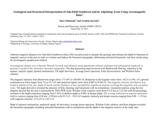
19. Figure 5. A. Grey shaded tilt derivative map. B. Color shaded tild derivative map of the study area.
20. Figure 6. Lineaments and archs marked out by Vectorisation.
840000850000860000870000880000
840000850000860000870000880000
60000 70000 80000 90000 100000 110000
60000 70000 80000 90000 100000 110000
7°50'
7°50'
2500 0 2500 5000 7500
(meters)
WGS 84 / UTM zone 32N
Scale 1:250000
maximum Amplitudes
Pseudo-gravity
28. Figure 14. Average power spectrums of aeromagnetic anomaly map indicating gradients used in calculating the average depth to the top of
magnetic sources.
29. Figure 15: Standard Euler solutions of Ado-Ekiti Southwest and its adjoining areas.
30. Figure 16. Windowed Euler solution map of Ado-Ekiti Southwest and its adjoining areas.
31. Table 1. The following table summarizes the structural indices for simple models in a magnetic field.
32. Table 2. Table showing the statistical report of the results of depth obtained.