SlideShare ist ein Scribd-Unternehmen logo
1 von 22
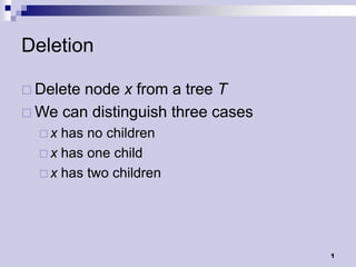
Deletion

 Deletenode x from a tree T
 We can distinguish three cases
  x  has no children
   x has one child
   x has two children


                                   1
Deletion Case 1
 If   x has no children – just remove x


                                           2
Deletion Case 2
 Ifx has exactly one child, then to delete
  x, simply make p[x] point to that child


                                              3
Deletion Case 3

 Ifx has two children, then
  to delete it we have to
    findits successor (or
     predecessor) y
    remove y (note that y has
     at most one child – why?)
    replace x with y


                                 4
Delete Pseudocode
 TreeDelete(T,z)
 01   if left[z]     NIL or right[z] = NIL
 02     then y     z
 03     else y     TreeSuccessor(z)
 04   if left[y]     NIL
 05     then x     left[y]
 06     else x     right[y]
 07   if x    NIL
 08     then p[x]      p[y]
 09   if p[y] = NIL
 10     then root[T]      x
 11     else if y = left[p[y]]
 12        then left[p[y]]     x
 13        else right[p[y]]      x
 14   if y    z
 15     then key[z]      key[y] //copy all fileds of y
 16   return y
                                                         5
In order traversal of a BST
 ITW can be thought of as a projection of
 the BST nodes onto a one dimensional
 interval


                                             6
BST Sorting
 Use TreeInsert and InorderTreeWalk to
 sort a list of n elements, A
   TreeSort(A)
   01 root[T]    NIL
   02 for i    1 to n
   03   TreeInsert(T,A[i])
   04 InorderTreeWalk(root[T])


                                          7
BST Sorting (2)
 Sort the following numbers
  5 10 7 1 3 1 8
 Build a binary search tree


   Call InorderTreeWalk

         1 1 3 5 7 8 10
                               8
In what order should we insert?
 We  want to sort numbers {1,2,…,n}
 Total time taken to insert these numbers
  equals the sum of the level numbers of the
  nodes.
 Thus if numbers were inserted in
  ascending order we would get a tree of
  height n-1 in which there is one node at
  each level.
 So total time for insertion in this case is
  1+2+3+…+n-1 = O(n2).
                                            9
Inserting a random permutation

 Suppose we take a random permutation of the
  keys and inserted them in this order.
 The total time required for insertion is now a
  random variable.
 We want to compute the expected value of this
  r.v.
 Recall that the expected value of a r.v. is the
  average value it takes over a large number of
  trials.
                                                    10
Expected insertion time for a random
permutation
 We  will compute the average time taken to
  insert keys in the order specified by the n!
  permutations.
 In other words, for each of the n!
  permutations we will compute the time
  taken to insert keys in that order and then
  compute the average.
 Let T(n) denote this quantity.


                                             11
Inserting a random permutation (2)

 Of the n! permutations, there are (n-1)!
  permutations in which the first element is i.
 The tree formed in these instances has i as
  the root. The left subtree has keys 1..(i-1)
  and the right subtree has keys (i+1)..n
 Consider the ordering of keys 1..(i-1) in the
  (n-1)! permutations. All (i-1)! permutations
  appear and each occurs (n-1)!/(i-1)! times.
                                              12
Inserting a random permuation(3)

 Recall   that if we only had keys 1..(i-1) then
  average time taken to insert them is T(i-1).
 The average is taken over all permutations
  of 1..(i-1).
 hence total time to insert all (i-1)!
  permutations is (i-1)!T(i-1).


                                               13
Inserting a random permutation(4)
 When    inserting keys 1..(i-1) into the left
  subtree, each key has to be compared with
  the root.
 This leads to an additional unit cost for each
  key.
 So total time to insert all (i-1)! permutations
  is (i-1)!(T(i-1)+(i-1)).
 Since each permutation appears (n-1)!/(i-1)!
  times, total time to insert keys 1..(i-1) is
  (n-1)!(T(i-1)+(i-1))
                                               14
Inserting a random permutation(5)
 Time  to insert keys 1..(i-1) is
  (n-1)!(T(i-1)+(i-1))
 Similarly, time to insert keys (i+1)..n is
  (n-1)!(T(n-i)+(n-i))
 Total time to insert all n keys in
  permutations where the first key is i is
  (n-1)! (T(i-1)+T(n-i)+ n-1)
 Total time to insert all n keys in all n!
  permutations is
  (n-1)! i=1n (T(i-1)+T(n-i)+ n-1).
                                               15
Building the recurrence


   We are expressing the value of function T() at
    point n in terms of the value of T() at points 0..n-
    1. This is called a recurrence relation.
                                                           16
Solving the recurrence


                         17
Solving the recurrence(2)


                            18
Summing the harmonic series
 What   is the sum ½+ 1/3 + ¼+…1/n?
      1/x


            1/2
               1/3
                  1/41/5           1/n
                        1/6
                                           x
            1 2 3 4 5 6              n
It is at most the area under the curve f(x)=1/x
between limits 1 and n                            19
The expected time for insertion


Thus the expected time for inserting a
randomly chosen permutation of n keys is
O(n log n)
                                           20
Minimum time to insert n keys
 The  time required to insert n keys is
  minimum when the resulting tree has the
  smallest possible height.
 A binary tree on n nodes has height at
  least log2 n
 To insert the n/2 nodes at level log2 n we
  require at least (n/2)log2 n time.
 Hence inserting n keys requires (nlog2 n)
  time.

                                           21
Summary of Running times
 To insert n keys into a binary search tree
  which is initially empty requires
 O(n2) time in the worst case.
 O(nlog n) time in the best case.
 O(nlog n) time in the average case; the
  average is taken over the n! different
  orders in which the n keys could be
  inserted.

                                               22

Weitere ähnliche Inhalte

Was ist angesagt? (20)

Lec11
Lec11Lec11
Lec11
 
Lec3
Lec3Lec3
Lec3
 
Lec5
Lec5Lec5
Lec5
 
Lec3
Lec3Lec3
Lec3
 
Lec20
Lec20Lec20
Lec20
 
Lec1
Lec1Lec1
Lec1
 
Animations tris
Animations trisAnimations tris
Animations tris
 
Récursivité
RécursivitéRécursivité
Récursivité
 
Red black tree
Red black treeRed black tree
Red black tree
 
skip list
skip listskip list
skip list
 
Lec2
Lec2Lec2
Lec2
 
Tree Data Structure by Daniyal Khan
Tree Data Structure by Daniyal KhanTree Data Structure by Daniyal Khan
Tree Data Structure by Daniyal Khan
 
Amortized Analysis
Amortized Analysis Amortized Analysis
Amortized Analysis
 
Quick sort algorithn
Quick sort algorithnQuick sort algorithn
Quick sort algorithn
 
Algorithmes d'approximation
Algorithmes d'approximationAlgorithmes d'approximation
Algorithmes d'approximation
 
Minimum spanning tree (mst)
Minimum spanning tree (mst)Minimum spanning tree (mst)
Minimum spanning tree (mst)
 
Python matplotlib cheat_sheet
Python matplotlib cheat_sheetPython matplotlib cheat_sheet
Python matplotlib cheat_sheet
 
fuzzy_measures.ppt
fuzzy_measures.pptfuzzy_measures.ppt
fuzzy_measures.ppt
 
Avl tree
Avl treeAvl tree
Avl tree
 
Time complexity
Time complexityTime complexity
Time complexity
 

Ähnlich wie Lec9

Skiena algorithm 2007 lecture09 linear sorting
Skiena algorithm 2007 lecture09 linear sortingSkiena algorithm 2007 lecture09 linear sorting
Skiena algorithm 2007 lecture09 linear sortingzukun
 
pradeepbishtLecture13 div conq
pradeepbishtLecture13 div conqpradeepbishtLecture13 div conq
pradeepbishtLecture13 div conqPradeep Bisht
 
Advanced data structure
Advanced data structureAdvanced data structure
Advanced data structureShakil Ahmed
 
Quicksort analysis
Quicksort analysisQuicksort analysis
Quicksort analysisPremjeet Roy
 
Skiena algorithm 2007 lecture08 quicksort
Skiena algorithm 2007 lecture08 quicksortSkiena algorithm 2007 lecture08 quicksort
Skiena algorithm 2007 lecture08 quicksortzukun
 
CS330-Lectures Statistics And Probability
CS330-Lectures Statistics And ProbabilityCS330-Lectures Statistics And Probability
CS330-Lectures Statistics And Probabilitybryan111472
 
Copy of y16 02-2119divide-and-conquer
Copy of y16 02-2119divide-and-conquerCopy of y16 02-2119divide-and-conquer
Copy of y16 02-2119divide-and-conquerJoepang2015
 
Review session2
Review session2Review session2
Review session2NEEDY12345
 
Show that the worst-case time complexity for Binary Search is given by.docx
Show that the worst-case time complexity for Binary Search is given by.docxShow that the worst-case time complexity for Binary Search is given by.docx
Show that the worst-case time complexity for Binary Search is given by.docxmmary455
 
Accurate, Simple and Efficient Triangulation of a Polygon by Ear Removal with...
Accurate, Simple and Efficient Triangulation of a Polygon by Ear Removal with...Accurate, Simple and Efficient Triangulation of a Polygon by Ear Removal with...
Accurate, Simple and Efficient Triangulation of a Polygon by Ear Removal with...Kasun Ranga Wijeweera
 
Unit-1 DAA_Notes.pdf
Unit-1 DAA_Notes.pdfUnit-1 DAA_Notes.pdf
Unit-1 DAA_Notes.pdfAmayJaiswal4
 
Fft presentation
Fft presentationFft presentation
Fft presentationilker Şin
 
PaperNo16-Habibi-IMF-On Syndetically Hypercyclic Tuples
PaperNo16-Habibi-IMF-On Syndetically Hypercyclic TuplesPaperNo16-Habibi-IMF-On Syndetically Hypercyclic Tuples
PaperNo16-Habibi-IMF-On Syndetically Hypercyclic TuplesMezban Habibi
 
Dynamical systems solved ex
Dynamical systems solved exDynamical systems solved ex
Dynamical systems solved exMaths Tutoring
 

Ähnlich wie Lec9 (20)

Lec9
Lec9Lec9
Lec9
 
Skiena algorithm 2007 lecture09 linear sorting
Skiena algorithm 2007 lecture09 linear sortingSkiena algorithm 2007 lecture09 linear sorting
Skiena algorithm 2007 lecture09 linear sorting
 
pradeepbishtLecture13 div conq
pradeepbishtLecture13 div conqpradeepbishtLecture13 div conq
pradeepbishtLecture13 div conq
 
Sorting
SortingSorting
Sorting
 
Advanced data structure
Advanced data structureAdvanced data structure
Advanced data structure
 
Lec16
Lec16Lec16
Lec16
 
Quicksort analysis
Quicksort analysisQuicksort analysis
Quicksort analysis
 
Skiena algorithm 2007 lecture08 quicksort
Skiena algorithm 2007 lecture08 quicksortSkiena algorithm 2007 lecture08 quicksort
Skiena algorithm 2007 lecture08 quicksort
 
CS330-Lectures Statistics And Probability
CS330-Lectures Statistics And ProbabilityCS330-Lectures Statistics And Probability
CS330-Lectures Statistics And Probability
 
2.pptx
2.pptx2.pptx
2.pptx
 
Copy of y16 02-2119divide-and-conquer
Copy of y16 02-2119divide-and-conquerCopy of y16 02-2119divide-and-conquer
Copy of y16 02-2119divide-and-conquer
 
Review session2
Review session2Review session2
Review session2
 
Show that the worst-case time complexity for Binary Search is given by.docx
Show that the worst-case time complexity for Binary Search is given by.docxShow that the worst-case time complexity for Binary Search is given by.docx
Show that the worst-case time complexity for Binary Search is given by.docx
 
Signals Processing Homework Help
Signals Processing Homework HelpSignals Processing Homework Help
Signals Processing Homework Help
 
Accurate, Simple and Efficient Triangulation of a Polygon by Ear Removal with...
Accurate, Simple and Efficient Triangulation of a Polygon by Ear Removal with...Accurate, Simple and Efficient Triangulation of a Polygon by Ear Removal with...
Accurate, Simple and Efficient Triangulation of a Polygon by Ear Removal with...
 
Unit-1 DAA_Notes.pdf
Unit-1 DAA_Notes.pdfUnit-1 DAA_Notes.pdf
Unit-1 DAA_Notes.pdf
 
Fft presentation
Fft presentationFft presentation
Fft presentation
 
Stirling theorem
Stirling theoremStirling theorem
Stirling theorem
 
PaperNo16-Habibi-IMF-On Syndetically Hypercyclic Tuples
PaperNo16-Habibi-IMF-On Syndetically Hypercyclic TuplesPaperNo16-Habibi-IMF-On Syndetically Hypercyclic Tuples
PaperNo16-Habibi-IMF-On Syndetically Hypercyclic Tuples
 
Dynamical systems solved ex
Dynamical systems solved exDynamical systems solved ex
Dynamical systems solved ex
 

Lec9

  • 1. Deletion  Deletenode x from a tree T  We can distinguish three cases x has no children  x has one child  x has two children 1
  • 2. Deletion Case 1  If x has no children – just remove x 2
  • 3. Deletion Case 2  Ifx has exactly one child, then to delete x, simply make p[x] point to that child 3
  • 4. Deletion Case 3  Ifx has two children, then to delete it we have to  findits successor (or predecessor) y  remove y (note that y has at most one child – why?)  replace x with y 4
  • 5. Delete Pseudocode TreeDelete(T,z) 01 if left[z] NIL or right[z] = NIL 02 then y z 03 else y TreeSuccessor(z) 04 if left[y] NIL 05 then x left[y] 06 else x right[y] 07 if x NIL 08 then p[x] p[y] 09 if p[y] = NIL 10 then root[T] x 11 else if y = left[p[y]] 12 then left[p[y]] x 13 else right[p[y]] x 14 if y z 15 then key[z] key[y] //copy all fileds of y 16 return y 5
  • 6. In order traversal of a BST  ITW can be thought of as a projection of the BST nodes onto a one dimensional interval 6
  • 7. BST Sorting  Use TreeInsert and InorderTreeWalk to sort a list of n elements, A TreeSort(A) 01 root[T] NIL 02 for i 1 to n 03 TreeInsert(T,A[i]) 04 InorderTreeWalk(root[T]) 7
  • 8. BST Sorting (2)  Sort the following numbers 5 10 7 1 3 1 8  Build a binary search tree  Call InorderTreeWalk 1 1 3 5 7 8 10 8
  • 9. In what order should we insert?  We want to sort numbers {1,2,…,n}  Total time taken to insert these numbers equals the sum of the level numbers of the nodes.  Thus if numbers were inserted in ascending order we would get a tree of height n-1 in which there is one node at each level.  So total time for insertion in this case is 1+2+3+…+n-1 = O(n2). 9
  • 10. Inserting a random permutation  Suppose we take a random permutation of the keys and inserted them in this order.  The total time required for insertion is now a random variable.  We want to compute the expected value of this r.v.  Recall that the expected value of a r.v. is the average value it takes over a large number of trials. 10
  • 11. Expected insertion time for a random permutation  We will compute the average time taken to insert keys in the order specified by the n! permutations.  In other words, for each of the n! permutations we will compute the time taken to insert keys in that order and then compute the average.  Let T(n) denote this quantity. 11
  • 12. Inserting a random permutation (2)  Of the n! permutations, there are (n-1)! permutations in which the first element is i.  The tree formed in these instances has i as the root. The left subtree has keys 1..(i-1) and the right subtree has keys (i+1)..n  Consider the ordering of keys 1..(i-1) in the (n-1)! permutations. All (i-1)! permutations appear and each occurs (n-1)!/(i-1)! times. 12
  • 13. Inserting a random permuation(3)  Recall that if we only had keys 1..(i-1) then average time taken to insert them is T(i-1).  The average is taken over all permutations of 1..(i-1).  hence total time to insert all (i-1)! permutations is (i-1)!T(i-1). 13
  • 14. Inserting a random permutation(4)  When inserting keys 1..(i-1) into the left subtree, each key has to be compared with the root.  This leads to an additional unit cost for each key.  So total time to insert all (i-1)! permutations is (i-1)!(T(i-1)+(i-1)).  Since each permutation appears (n-1)!/(i-1)! times, total time to insert keys 1..(i-1) is (n-1)!(T(i-1)+(i-1)) 14
  • 15. Inserting a random permutation(5)  Time to insert keys 1..(i-1) is (n-1)!(T(i-1)+(i-1))  Similarly, time to insert keys (i+1)..n is (n-1)!(T(n-i)+(n-i))  Total time to insert all n keys in permutations where the first key is i is (n-1)! (T(i-1)+T(n-i)+ n-1)  Total time to insert all n keys in all n! permutations is (n-1)! i=1n (T(i-1)+T(n-i)+ n-1). 15
  • 16. Building the recurrence  We are expressing the value of function T() at point n in terms of the value of T() at points 0..n- 1. This is called a recurrence relation. 16
  • 19. Summing the harmonic series  What is the sum ½+ 1/3 + ¼+…1/n? 1/x 1/2 1/3 1/41/5 1/n 1/6 x 1 2 3 4 5 6 n It is at most the area under the curve f(x)=1/x between limits 1 and n 19
  • 20. The expected time for insertion Thus the expected time for inserting a randomly chosen permutation of n keys is O(n log n) 20
  • 21. Minimum time to insert n keys  The time required to insert n keys is minimum when the resulting tree has the smallest possible height.  A binary tree on n nodes has height at least log2 n  To insert the n/2 nodes at level log2 n we require at least (n/2)log2 n time.  Hence inserting n keys requires (nlog2 n) time. 21
  • 22. Summary of Running times  To insert n keys into a binary search tree which is initially empty requires  O(n2) time in the worst case.  O(nlog n) time in the best case.  O(nlog n) time in the average case; the average is taken over the n! different orders in which the n keys could be inserted. 22