SlideShare ist ein Scribd-Unternehmen logo
1 von 46
Department of Mechanical Engineering
University of Washington
Stevens Way, Box 352600
Seattle, WA 98195 USA
206-543-5090
Reaction Wheel Controlled 2D Cubli
Reese Taylor
reeset1@uw.edu
Sayed Torak
itorak@uw.edu
Austin Sanchez
aksanch@uw.edu
Gabe Weight
weightgc@uw.edu
Kirim Lee
kirim13@uw.edu
ME 495 Report — June 10, 2022
1
Contents
1 Executive Summary 5
2 Introduction 5
2.1 Project Definition . . . . . . . . . . . . . . . 5
2.2 Functional Specifications . . . . . . . . . . . 5
2.3 Design approach . . . . . . . . . . . . . . . 6
3 Dynamic Model 6
3.1 Non-Linear Model . . . . . . . . . . . . . . 6
3.2 Linearized Model . . . . . . . . . . . . . . . 7
4 Control Overview 7
4.1 PI Controller . . . . . . . . . . . . . . . . . 8
4.2 Linear Quadratic Integral Controller . . . . 8
5 Simulation Design 8
5.1 Parameter Estimation . . . . . . . . . . . . 9
5.2 Linear vs Non-Linear Model . . . . . . . . . 9
5.3 Jump-up Modeling . . . . . . . . . . . . . . 9
5.4 Current Step Disturbance . . . . . . . . . . 10
5.5 Recovery Angle . . . . . . . . . . . . . . . . 10
6 Prototype Design 11
6.1 Purpose . . . . . . . . . . . . . . . . . . . . 11
6.2 Critical Component Selection . . . . . . . . 11
6.2.1 Motor . . . . . . . . . . . . . . . . . 11
6.2.2 Motor Controller . . . . . . . . . . . 12
6.2.3 Servo . . . . . . . . . . . . . . . . . 12
6.2.4 Collet Prop Adapter . . . . . . . . . 12
6.2.5 IMU . . . . . . . . . . . . . . . . . . 13
6.3 Mechanical Design . . . . . . . . . . . . . . 13
6.3.1 Frame and Motor Cantilever . . . . 13
6.3.2 Flywheel . . . . . . . . . . . . . . . 13
6.3.3 Braking System . . . . . . . . . . . . 14
6.3.4 CAD Model . . . . . . . . . . . . . . 14
6.3.5 Manufacturing . . . . . . . . . . . . 15
6.4 Electrical Design . . . . . . . . . . . . . . . 15
6.4.1 NI myRio-1900 . . . . . . . . . . . . 15
6.4.2 Power Supply . . . . . . . . . . . . . 15
6.4.3 Servo Battery . . . . . . . . . . . . . 15
6.4.4 Encoder . . . . . . . . . . . . . . . . 16
6.5 Computational Design . . . . . . . . . . . . 16
6.5.1 Complementary Filter . . . . . . . . 16
6.5.2 Finite State Machine . . . . . . . . . 17
6.5.3 Off State . . . . . . . . . . . . . . . 18
6.5.4 Speed Up State . . . . . . . . . . . . 18
6.5.5 Brake State . . . . . . . . . . . . . . 18
6.5.6 Brake to Balance State . . . . . . . 18
6.5.7 Balance State . . . . . . . . . . . . . 18
6.6 Final Assembly . . . . . . . . . . . . . . . . 18
7 Testing 18
7.1 IMU vs Encoder . . . . . . . . . . . . . . . 18
7.2 Current Disturbance Response . . . . . . . 19
7.3 Jump Up Response . . . . . . . . . . . . . . 19
7.4 Max Recovery Response . . . . . . . . . . . 20
7.5 Hall Sensor Issue . . . . . . . . . . . . . . . 20
7.6 Comparison to Functional Specifications . . 21
8 Risk and Liability 21
9 Ethical Issues 22
10 Impact on Society 22
11 Impact on the Environment 22
12 Cost and Engineering Economics 22
13 Codes and Standards 23
14 Conclusions 23
14.1 Continued development . . . . . . . . . . . 23
14.2 Final product configuration . . . . . . . . . 23
15 Appendix 25
15.A Simulink Block Diagrams . . . . . . . . . . 25
15.B Manufacturing Drawings . . . . . . . . . . . 29
15.C Wiring Diagram . . . . . . . . . . . . . . . 35
15.D Code . . . . . . . . . . . . . . . . . . . . . . 36
15.D.1 Main Thread Diagram . . . . . . . . 36
15.D.2 IRQ Timer Thread Diagram . . . . 37
15.E Component Specification Sheets . . . . . . . 38
15.E.1 Motor Specifications . . . . . . . . . 38
15.E.2 Motor Controller Specifications . . . 40
2
List of Figures
1 Cubli Body Free Body Diagram . . . . . . . . . . . . . . . . . . . . . . . . . . . . . . . . . . . . . . . . . . 6
2 Cubli Wheel Free Body Diagram . . . . . . . . . . . . . . . . . . . . . . . . . . . . . . . . . . . . . . . . . 7
3 Nonlinear Cubli Plant Model . . . . . . . . . . . . . . . . . . . . . . . . . . . . . . . . . . . . . . . . . . . 7
4 PI Control Loop . . . . . . . . . . . . . . . . . . . . . . . . . . . . . . . . . . . . . . . . . . . . . . . . . . 8
5 LQI Control Loop . . . . . . . . . . . . . . . . . . . . . . . . . . . . . . . . . . . . . . . . . . . . . . . . . 8
6 Comparison of Linear and Nonlinear Systems . . . . . . . . . . . . . . . . . . . . . . . . . . . . . . . . . . 9
7 Simulated Jump Up Response . . . . . . . . . . . . . . . . . . . . . . . . . . . . . . . . . . . . . . . . . . . 9
8 Simulated current disturbance state variable response . . . . . . . . . . . . . . . . . . . . . . . . . . . . . 10
9 Simulated controller current response . . . . . . . . . . . . . . . . . . . . . . . . . . . . . . . . . . . . . . . 11
10 Simulated 2◦
recovery angle response . . . . . . . . . . . . . . . . . . . . . . . . . . . . . . . . . . . . . . . 11
11 Maxon EC 45 Flat 70W Brushless DC Motor . . . . . . . . . . . . . . . . . . . . . . . . . . . . . . . . . . 12
12 ESCON 36/3 EC Motor Controller . . . . . . . . . . . . . . . . . . . . . . . . . . . . . . . . . . . . . . . . 12
13 Reefs RC 99 Micro . . . . . . . . . . . . . . . . . . . . . . . . . . . . . . . . . . . . . . . . . . . . . . . . . 13
14 Collet Prop Adapter . . . . . . . . . . . . . . . . . . . . . . . . . . . . . . . . . . . . . . . . . . . . . . . . 13
15 SparkFun LSM9DS1 9DOF IMU . . . . . . . . . . . . . . . . . . . . . . . . . . . . . . . . . . . . . . . . . 13
16 Frame CAD Render . . . . . . . . . . . . . . . . . . . . . . . . . . . . . . . . . . . . . . . . . . . . . . . . 14
17 Flywheel CAD Render . . . . . . . . . . . . . . . . . . . . . . . . . . . . . . . . . . . . . . . . . . . . . . . 14
18 Braking System CAD Render - Back View . . . . . . . . . . . . . . . . . . . . . . . . . . . . . . . . . . . . 14
19 Braking System CAD Render - Front View . . . . . . . . . . . . . . . . . . . . . . . . . . . . . . . . . . . 14
20 Final Prototype CAD Render . . . . . . . . . . . . . . . . . . . . . . . . . . . . . . . . . . . . . . . . . . . 15
21 Final Prototype CAD Render - Top View . . . . . . . . . . . . . . . . . . . . . . . . . . . . . . . . . . . . 15
22 Reaction Wheel Manual CNC Manufacturing . . . . . . . . . . . . . . . . . . . . . . . . . . . . . . . . . . 15
23 NI myRio-1900 Embedded Computer . . . . . . . . . . . . . . . . . . . . . . . . . . . . . . . . . . . . . . . 16
24 24V Mean Well power supply with 12.5A output . . . . . . . . . . . . . . . . . . . . . . . . . . . . . . . . 16
25 6V 1600mAh RC Servo Battery . . . . . . . . . . . . . . . . . . . . . . . . . . . . . . . . . . . . . . . . . . 16
26 US Digital S2-2000-B Optical Quadrature Encoder . . . . . . . . . . . . . . . . . . . . . . . . . . . . . . . 16
27 Complementary Filter Block Diagram . . . . . . . . . . . . . . . . . . . . . . . . . . . . . . . . . . . . . . 16
28 Complementary Filter Bode Plot . . . . . . . . . . . . . . . . . . . . . . . . . . . . . . . . . . . . . . . . . 17
29 State Transition Diagram . . . . . . . . . . . . . . . . . . . . . . . . . . . . . . . . . . . . . . . . . . . . . 17
30 Final Assembly . . . . . . . . . . . . . . . . . . . . . . . . . . . . . . . . . . . . . . . . . . . . . . . . . . . 18
31 Encoder vs IMU response . . . . . . . . . . . . . . . . . . . . . . . . . . . . . . . . . . . . . . . . . . . . . 19
32 5A current disturbance state variable response . . . . . . . . . . . . . . . . . . . . . . . . . . . . . . . . . 19
33 Controller current response . . . . . . . . . . . . . . . . . . . . . . . . . . . . . . . . . . . . . . . . . . . . 19
34 Jump Up to Balancing Response . . . . . . . . . . . . . . . . . . . . . . . . . . . . . . . . . . . . . . . . . 20
35 Maximum Recovery Angle Response . . . . . . . . . . . . . . . . . . . . . . . . . . . . . . . . . . . . . . . 20
36 Hall Sensor Issue - Actual vs Measured Wheel Velocity . . . . . . . . . . . . . . . . . . . . . . . . . . . . . 21
37 Simulated jump up response using recorded wheel data . . . . . . . . . . . . . . . . . . . . . . . . . . . . . 21
38 Full Simulink Block Diagram . . . . . . . . . . . . . . . . . . . . . . . . . . . . . . . . . . . . . . . . . . . 25
39 Cubli Plant Simulink Model . . . . . . . . . . . . . . . . . . . . . . . . . . . . . . . . . . . . . . . . . . . . 26
40 Simulink Braking System . . . . . . . . . . . . . . . . . . . . . . . . . . . . . . . . . . . . . . . . . . . . . 27
41 Simulink PI Speed Controller . . . . . . . . . . . . . . . . . . . . . . . . . . . . . . . . . . . . . . . . . . . 27
42 Simulink LQI Balance Controller . . . . . . . . . . . . . . . . . . . . . . . . . . . . . . . . . . . . . . . . . 28
43 Frame Drawing File . . . . . . . . . . . . . . . . . . . . . . . . . . . . . . . . . . . . . . . . . . . . . . . . 29
44 Cantilever Base Drawing File . . . . . . . . . . . . . . . . . . . . . . . . . . . . . . . . . . . . . . . . . . . 30
45 Cantilever Motor Mount Drawing File . . . . . . . . . . . . . . . . . . . . . . . . . . . . . . . . . . . . . . 31
46 Flywheel Drawing File . . . . . . . . . . . . . . . . . . . . . . . . . . . . . . . . . . . . . . . . . . . . . . . 32
47 Caliper Drawing File . . . . . . . . . . . . . . . . . . . . . . . . . . . . . . . . . . . . . . . . . . . . . . . . 33
48 Servo Mount Drawing File . . . . . . . . . . . . . . . . . . . . . . . . . . . . . . . . . . . . . . . . . . . . . 34
49 Wiring Diagram . . . . . . . . . . . . . . . . . . . . . . . . . . . . . . . . . . . . . . . . . . . . . . . . . . 35
50 Main Thread Flowchart . . . . . . . . . . . . . . . . . . . . . . . . . . . . . . . . . . . . . . . . . . . . . . 36
51 Timer IRQ Thread Flowchart . . . . . . . . . . . . . . . . . . . . . . . . . . . . . . . . . . . . . . . . . . . 37
3
List of Tables
1 Functional Specifications . . . . . . . . . . . . . . . . . . . . . . . . . . . . . . . . . . . . . . . . . . . . . . 6
2 List of Symbols . . . . . . . . . . . . . . . . . . . . . . . . . . . . . . . . . . . . . . . . . . . . . . . . . . . 6
3 List of Parameters . . . . . . . . . . . . . . . . . . . . . . . . . . . . . . . . . . . . . . . . . . . . . . . . . 9
4 EC 45 Flat 70W specifications . . . . . . . . . . . . . . . . . . . . . . . . . . . . . . . . . . . . . . . . . . 12
5 ESCON 36/3 EC Specifications . . . . . . . . . . . . . . . . . . . . . . . . . . . . . . . . . . . . . . . . . . 12
6 Reefs RC 99 Micro Specifications . . . . . . . . . . . . . . . . . . . . . . . . . . . . . . . . . . . . . . . . . 12
7 Comparison to Functional Specifications . . . . . . . . . . . . . . . . . . . . . . . . . . . . . . . . . . . . . 21
8 Purchase list . . . . . . . . . . . . . . . . . . . . . . . . . . . . . . . . . . . . . . . . . . . . . . . . . . . . 23
4
1 Executive Summary
The three-dimensional Cubli is a reaction wheel con-
trolled inverted pendulum system that is capable of balanc-
ing itself on an edge or corner as well as jumping itself up
to a balance position from flat on a table. This report de-
scribes the design process, dynamic modeling, simulation,
physical implementation, testing, and results of building a
two-dimension prototype of the full Cubli system. It com-
pares the results of simulation predictions to that of the
physical prototype for several distinct testing procedures,
justifies the differences, and discusses areas of improvement
for future iterations.
A mathematical model of the two-dimensional Cubli dy-
namic system was derived from basic equations of motion
and physics relationships, and two different linear con-
trollers were developed to control the speed of the fly-
wheel and to balance the system about a corner based
on this model. The controllers were designed to meet
the functional specifications outlined at the start of the
project. The model and controllers were then simulated
using Simulink and a MATLAB script to predict the be-
havior of the system during a jump up process, a current
disturbance, and an angle initial condition response.
Several components of the prototype were manufactured
in the ME machine shop out of available aluminum stock
material. These components included the frame, flywheel,
braking system, and motor cantilever mounts, all of which
were designed in Solidworks to maximize strength and min-
imize weight, while providing robust connections between
critical components.
State estimation and feedback was accomplished via a
Sparkfun 9Dof Inertial Measurement Unit (IMU) to mea-
sure the angle and angular velocity of the cubli body, and
Hall sensors built into the flywheel motor to measure the
angular velocity of the wheel. The use of an IMU over an
encoder for angle measurements allowed the system to stay
balanced while the orientation of the supporting base is
changed. A complementary filter was implemented to pro-
vide a more accurate estimation of the angle of the body
by combining data from both the accelerometers and gy-
roscopes.
The computational control and data collection for the
system were accomplished using a program built in C run-
ning on a myRIO-1900 embedded computer. This com-
puter communicates with the Cubli prototype to estimate
the current state via the IMU and Hall sensors, provide
current to the motor to speed up the flywheel, and con-
trol the orientation of an RC servo to actuate the braking
system. The Maxon EC 45 Flat 70W Brushless DC motor
was controlled using an ESCON 36/3 EC 4-quadrant mo-
tor controller that received analog set values for the desired
motor current from the myRIO-1900. The RC servo motor
orientation was controlled by adjusting the duty cycle of
a Pulse Width Modulated (PWM) signal sent to the servo
motor via the myRIO-1900.
The C program integrates this state estimation with a fi-
nite state machine to control the current sent to the Cubli
prototype and the transition between five distinct states
including an off state, a speed up state, a brake state, a
brake to balance state, and a balancing state. The state
machine relies on a separate Timer IRQ thread for timing
with a sample rate of 5ms, and the transitions are con-
trolled by conditions related to the current state variables,
keypad button presses, and timing variables.
A final prototype was assembled and several tests were
conducted to compare the simulated dynamic behavior to
the real world behavior. These tests included jump up to
balance tests, a 5A forced current disturbance test, and
a maximum recovery angle test, all of which showed close
agreement between the simulated and real results. Fur-
ther analysis was presented to quantify the difference be-
tween the simulation predictions and actual results, and
limiting issues were identified and discussed. Final conclu-
sions were presented that consider the overall success of
the project and recommended directions in which future
iterations should proceed.
2 Introduction
2.1 Project Definition
The Cubli is a reaction wheel controlled inverted pendu-
lum system in the shape of a cube and was first developed
by The Institute for Dynamic Systems and Control at ETH
Zurich university [1]. The system is capable of transferring
momentum stored in the three actively controlled onboard
flywheels to the external frame via a mechanical braking
system, allowing it to jump up from a face onto an edge or
corner and actively balance while rejecting disturbances.
The goal of this capstone project is to design and develop
a functioning two-dimensional prototype of the full three-
dimensional Cubli with only one rotational degree of free-
dom. This prototype will be able to jump up from its edge
to a corner and actively balance in an unstable position by
applying torque to the system’s flywheel. The design will
include a mechanical braking system, a PI speed controller
to initiate the momentum transferring jump up procedure,
and an LQI state feedback controller to actively balance
the system on a corner.
2.2 Functional Specifications
To aid in a successful project, the following quantitative
functional specifications were set as target goals for the
final prototype.
5
Table 1: Functional Specifications
Jump up success rate >95 %
Maximum recovery angle >7◦
Total mass <1 kg
Recovery overshoot <75 %
Recovery settling time <3 s
Steady state error <1◦
2.3 Design approach
The main considerations for the prototype design were
scope and performance. Firstly, the scope of this project
was limited to a two-dimensional Cubli system to allow
for full completion within the two quarter timeline. This
led to prioritizing simplicity where possible, such as in the
braking system and flywheel design. With additional time
and resources, the final prototype presented in this report
can be easily extrapolated to build a full three-dimensional
Cubli system without much additional effort, since the de-
sign and control for a single rotational degree of freedom
has already been achieved.
Secondly, the prototype was designed to meet or exceed
the functional specifications listed above. One key consid-
eration to accomplish this was the sizing of the system and
the various components used. The mass of the system was
limited to less than one kilogram as to require less angular
velocity and torque from the motor to effectively jump up
to the corner and correct for disturbances. So the system
was sized accordingly to accomplish this. Furthermore, re-
liability was a major consideration while developing the
final prototype. A jump up success rate greater than 95%
was desired, so the design for the final prototype was based
mainly on minimizing weight and maximizing reliability.
3 Dynamic Model
3.1 Non-Linear Model
The dynamic model of the cubli is based on the deriva-
tions presented in [2] and [3]. The equations of motion
for the system are derived from the free body diagrams of
the cubli body and flywheel shown in Figures 1 and 2 re-
spectively, and the parameters used in this derivation are
summarized in Table 2. The flywheel is supported directly
by the cubli body, which can rotate independently of the
flywheel, so it is necessary to specify the angle of the wheel
with respect to the angle of the body for this derivation,
as shown in Figure 2.
The cubli body is subjected to external torques from
gravity and the motor as well as damping torques from
the motor and pivot bearings. In the reference frame of the
Table 2: List of Symbols
Symbol Definition Units
θb Body angle rad
θ̇b Body angular velocity rad
s
θ̈b Body angular acceleration rad
s2
θ̇w Wheel angular velocity rad
s
θ̈w Wheel angular acceleration rad
s2
Bb Body damping N·m·s
rad
Bw Wheel damping N·m·s
rad
mb Body mass kg
mw Wheel mass kg
lw Pivot to wheel center m
lb Pivot to center of mass m
τm Motor torque N · m
Iw Wheel inertia kg · m2
Ib Body inertia kg · m2
KKm Motor Constant Nm
A
cubli body, the flywheel is subjected to equal and opposite
bearing and motor torques as well as an external force of
gravity that causes a torque on the body.
Figure 1: Cubli Body Free Body Diagram
The equation of motion for the cubli body is summarized
in (1). Rewriting the torque terms in this equation to be
in terms of the body angle, body angular velocity, and
wheel angular velocity yields an expression for the angular
acceleration of the body, shown in (2).
6
Figure 2: Cubli Wheel Free Body Diagram
(Ib + mwlw
2
)θ̈b = τBb
+ τg + τBw
− τm (1)
θ̈b =
−Bbθ̇b + (mblb + mwlw)g · sin(θb) + Bwθ̇w − τm
Ib + mwlw
2
(2)
The equation for the angular acceleration of the flywheel
is shown in (3), which directly depends on the angular
acceleration of the cubli body due to the flywheel angle
dependency on the angle of the body. From (2) and (3),
the nonlinear block diagram of the cubli body is derived
and shown in Figure 3. This model is set up as a single
input multiple output system, since our strategy to control
this system during balancing is based on the principles of
full state control, thus requiring all state variables of the
system as outputs.
θ̈w =
τm − Bwθ̇w − ¨
θb
Iw
(3)
3.2 Linearized Model
Next, the nonlinear cubli plant model can be linearized
about the operating point of θb = 0 using a small angle
approximation so that sin(θb) ≈ θb. This removes the sin
term from the plant model and allows for the derivation of
a state space representation of our model in the form shown
in (4) that is used in designing the balancing controller.
Here the state vector of this system, x, is composed the
angle of the cubli body, θb, the angular velocity of the body,
θ̇b, and the angular velocity of the flywheel, θ̇w. The single
Figure 3: Nonlinear Cubli Plant Model
input to this system, u, is the current delivered to the
motor. These expressions are summarized in (5). Finally,
the A and B matrices are derived from the cubli plant
model and shown in (6) and (7).
ẋ = Ax + Bu, y = x (4)
x =





θb
θ̇b
θ̇w





, u =
h
im
i
(5)
A =






0 1 0
(mblb+mwlw)g
Ib+mwlw
2 − Bb
Ib+mwlw
2
Bw
Ib+mwlw
2
−(mblb+mwlw)g
Ib+mwlw
2
Bb
Ib+mwlw
2 −
Bw(Ib+Iw+mwlw
2
)
Iw(Ib+mwlw
2)






(6)
B =






0
− Km
Ib+mwlw
2
Km(Ib+Iw+mwlw
2
)
Iw(Ib+mwlw
2)






(7)
4 Control Overview
Two separate controllers were used to control the Cubli
prototype. A proportional-integral (PI) controller was de-
veloped to control the angular velocity of the flywheel to a
desired speed prior to braking. A linear quadratic integral
controller (LQI) was developed to control all three state
variables of the system simultaneously to achieve robust
balancing performance. For both controllers, the output
of the controller is a current sent directly to the motor
7
controller operating in current controller mode. This al-
lows for direct control of the torque applied to the motor
in both cases.
4.1 PI Controller
Figure 4: PI Control Loop
The control loop for the PI speed controller is shown
above in Figure 4. Here, the controller is only controlling
the angular velocity of the flywheel, θ̇w, and not the other
state variables. This controller is the same controller used
in Lab 7 of ME 477 at the University of Washington, which
is used to control the speed of a DC motor and inertial
load. It is based on the continuous PI controller transfer
function shown in the left box of Figure 4. This continuous
controller transfer function was discretized using Tustin’s
method and implemented with a linear difference equation
using the function cascade() in the C control code.
The final values of the proportional gain and integral
gain terms in this transfer function are Kp = 0.25 Ki =
0.125. These were selected through iteration to achieve
a fast speed up from 0 RPM to the desired angular ve-
locity with minimal overshoot. To further minimize the
overshoot of the speed up process, the function sramps()
was implemented to create an angular velocity trajectory
as the reference input, rather than a large step change.
4.2 Linear Quadratic Integral Controller
Figure 5: LQI Control Loop
The control loop for the Linear Quadratic Integral (LQI)
feedback controller is shown above in Figure 5. This type of
controller is similar to a linear quadratic regulator (LQR)
that minimizes a cost function J to find the optimal gain
matrix, K, given a set of system and power costs. The key
difference between these control types is that the LQI con-
troller augments the original state space representation of
the Cubli system with an additional state z =
R t
0
(r−y)dτ,
representing the integral of the error signal for the wheel
angular velocity, θw. This helps to drive the steady state
error of the system to zero if there are errors between the
dynamic model and real prototype parameters. The result-
ing augmented state space model is shown below in equa-
tion 8, where C = [ 0, 0, 1 ]. This type of controller
was selected because of its ease of use and implementation
and suitability for controlling a system in state space form.

ẋ
ż

=

A 0
−C 0
 
x
z

+

B
0

u +

0
I

r (8)
Parameters such as performance (e.g. how quickly re-
sponse returns to desired state) and effort (e.g. actuation
effort) are optimized by the user defined matrices Q and
R. These cost matrices were first selected using Bryson’s
rule, where (xi)max and (ui)max are the largest reasonable
input magnitudes for each state and input variable respec-
tively, arranged along the diagonal of each matrix raised
to the power of negative 2. These values were then tuned
iteratively to achieve the best balancing performance, and
the final cost matrices used are shown in 9 and 10.
Q =






(1)−2
0 0 0
0 (5)−2
0 0
0 0 (2.7)−2
0
0 0 0 (15)−2






(9)
R =

(0.92)−2

(10)
The lqi() function in MATLAB was then used to cal-
culate the optimal gain matrix, K, by minimizing the
quadratic cost function J in (11) with the defined cost ma-
trices Q and R. This gain matrix can be represented by
K = [ Kp, Ki ], where the Kp terms represent the LQR
gain matrix, and the Ki term represents the gain for the
integral state. The optimal gain matrix used in the final
prototype is shown in 12. The controller was then imple-
mented into the C control code following the control loop
in Figure 5.
J =
Z ∞
0
(
h
xT
zT
i
Q

x
z
#
+ uT
Ru dt (11)
K =

−144.4222 −19.8352 −0.3611 0.0613

(12)
5 Simulation Design
A Simulink model in conjunction with a MATLAB script
was developed to predict the dynamic performance of the
system and speed/balance controllers used in the final pro-
totype. The Simulink model is composed of the Cubli plant
8
model shown in Figure 3, along with a LQI balance con-
troller, PI speed controller, braking system, and logic to
control the transitions between initiating the momentum
transfer for the jump up and the balancing control. De-
tailed images of these various block diagrams can be found
in Figures 38 - 42 in Appendix A.
5.1 Parameter Estimation
The parameters used in the Simulink model and MAT-
LAB script were based on the actual parameters of the final
prototype, which were determined in two ways. Firstly, the
mass of the body, mb, and the mass of the wheel, mw, were
measured directly after full prototype assembly, along with
the length from the pivot to the center of the wheel, lw.
Since precision bearings were used for both the body and
wheel, the respective damping coefficients were very small
and assumed to be zero. The remaining parameters were
based on Solidworks inertia analysis on the final updated
CAD model after adjusting the masses to match what was
measured directly. The resulting parameters are shown in
Table 3 below, which were used in all simulation results
presented in this report.
Table 3: List of Parameters
Symbol Value Units
mw 0.2201 kg
lw 0.0955 m
Iw 7.221 × 10⁻⁴
kg · m2
Bw 0 N·m·s
rad
mb 0.6123 kg
lb 0.0934 m
Ib 0.0119 kg · m2
Bb 0 N·m·s
rad
5.2 Linear vs Non-Linear Model
Figure 6 presents a simulated comparison between the
non-linear dynamic model and linearized state space model
for an initial condition response of θb = 5◦
. This response
has no external torque input from the motor, so the re-
sponse is expected to be unstable about θb = 0◦
and stable
about θb = 180◦
, which is the exact behavior predicted by
the simulation.
Comparing the nonlinear initial condition simulation to
the linearized approximation reveals that the linear ap-
proximation for all state variables is extremely close to the
nonlinear behavior up to an angle of θb ≈ 45◦
at t ≈ 0.3
sec. This indicates that the body angle range where the
linear model closely approximates the non-linear model is
much larger than the target control range for the LQI con-
troller. The full range of motion of the final prototype is
limited to ±45◦
, and the LQI is only intended to operate
over a portion of this range, so the performance of the lin-
earized LQI controller should not be severely affected by
deviation from the target angle of 0◦
.
Figure 6: Comparison of Linear and Nonlinear Systems
5.3 Jump-up Modeling
Figure 7: Simulated Jump Up Response
The jump-up procedure for the two-dimensional Cubli
9
is achieved by increasing the velocity of the flywheel to
a specified angular speed and rapidly braking the wheel
along the outer edge. The braking mechanism is fixed to
the body so that upon initiation of the braking, the mo-
mentum of the wheel is transferred to the body via the
friction force between the brake pads and the wheel sur-
face.
The Simulink model for the braking system is split into
two sections. The first section simulates a supporting force
on the body while the system is stationary. In real life, the
body would be resting on a table surface prior to initiating
the jump up procedure, which limits the body angle to ±
45◦
and prevents the body from moving as the wheel ac-
celerates. This behavior is not captured by the differential
equations, so to model this, all active accelerations signals
were identified and fed back into the system as negative
signals. This allows the simulation to accelerate the fly-
wheel to the desired speed while maintaining the angle of
the body at 45◦
.
The next section in the braking model is used to slow
down the wheel and transfer momentum to the body. This
is achieved by introducing equal and opposite external
torques to the body and wheel that represent the torque
applied to the wheel and body by a mechanical braking
system. To apply the torques appropriately, a group of
logic operators were implemented to the Simulink model
that check if enough momentum is transferred to the body
to lift it off the table. The logic operators then turn off
all table support signals and keep the momentum transfer
signal active. Once the angle of the body reaches a speci-
fied angle, the LQI controller is activated and the system
is balanced.
This Simulink model was used to accurately compute
the minimum angular velocity of the flywheel required for
some specified final jump-up angle based on an approx-
imate impulse in the braking force applied to the wheel.
The approximate impulse function was applied using a step
pulse with an extremely small width and large amplitude,
to simulate the conditions of a perfect impulse. The model
developed was compared against theoretical speeds that
were calculated using (13), which is derived from a per-
fectly inelastic momentum transfer between the wheel and
body [3].
ω2
w = (2 −
√
2)
Iw + Ib + mwl2
w

I2
w
(mblb + mwlw) ge (13)
Equation 12 predicts a wheel velocity of θ̇w = -1073.6
RPM to bring the body from an initial angle of 45◦
ex-
actly to 0◦
. Our simulation results predict θ̇w ≈ -1090
RPM to bring the body angle from an initial angle of 45◦
to nearly 0◦
, which is extremely close to that of the perfect
momentum transfer as well as the actual jump up speed
selected for the final prototype of -1080 RPM. The sim-
ulation plots of the state variable jump up and balance
response are shown in Figure 7.
5.4 Current Step Disturbance
Figure 8: Simulated current disturbance state variable re-
sponse
Figures 8 and 9 presents a simulated current disturbance
response. In this, an external current disturbance of 5A is
added to the LQI controller current output that is sent
to the non-linear Cubli plant model. The simulation then
predicts the state variable responses to this current dis-
turbance as well as the controller current output, current
sent to the motor, and resulting motor torque. Note that
the controller current output settles at a value of -5A to
exactly cancel with the 5A disturbance, resulting in zero
current and zero torque sent to the motor in steady state.
5.5 Recovery Angle
Figure 10 shows a simulated 2◦
recovery angle balancing
response for each state variable. In this, the initial body
angle was set to θb = 2◦
, and the initial body and wheel
velocities were set to zero. This imitates the LQI controller
response to a 2◦
step change in the reference angle.
10
Figure 9: Simulated controller current response
Figure 10: Simulated 2◦
recovery angle response
6 Prototype Design
6.1 Purpose
The main purpose of this prototype was to compare the
simulation predictions with a real life prototype to verify
both the simulation results and final design. Additionally,
the purpose of this prototype was to explore and imple-
ment mechatronics concepts in a hands-on context. Creat-
ing a physical prototype presented challenges in manufac-
turing, assembly, and moving from theoretical concepts to
their practical application. This prototype was an oppor-
tunity to move beyond the classroom and gain real-world
engineering experience.
Furthermore, this prototype also served as a proof-of-
concept and starting point for development of a full 3D
Cubli prototype. The scope of a fully 3D Cubli prototype
from scratch is too large to complete in two quarters, so
this prototype can be viewed directly as a starting point
for developing the full Cubli system.
6.2 Critical Component Selection
The final prototype has several critical components that
are necessary for proper operation of the two-dimensional
Cubli. These include the motor, motor controller, RC
servo motor, collet propeller adapter, and inertia measure-
ment unit. More detail is provided for each of these com-
ponents in the following sections.
A useful method used in selecting these final components
was examining the choices made by other Cubli projects.
Several papers that included detailed lists of which parts
were used and why they were selected [1][4][5][2][6], which
provided valuable resources to draw ideas from initially.
The search was then narrowed to fit the desired functional
specifications and ensure compatibility between compo-
nents.
6.2.1 Motor
The motor for the final prototype is the Maxon EC 45
Flat 70W Brushless DC motor. This motor has built in
Hall sensors for commutation and measurement of angular
velocity directly, which was a critical aspect for the feed-
back control system. An image of the motor and some
important specifications are shown below in Figure 11 and
Table 4.
One difficulty confronted during motor selection is the
trade-off between torque and angular velocity. Motors that
are geared to have high output torque have low operating
speeds and those meant to operate at high speed have low
torque output. Further complicating the choice was the
need to keep the mass and volume as low as possible for
each component. The EC 45 Flat 70W motor has a good
combination of high torque and high speeds while minimiz-
ing weight, so it was an ideal choice to control the flywheel
without adding unnecessary mass or requiring excessive
power consumption.
11
Figure 11: Maxon EC 45 Flat 70W Brushless DC Motor
Table 4: EC 45 Flat 70W specifications
Parameter Spec Units
Nominal Voltage 24 V
Nominal speed 4860 rpm
Nominal torque 128 mN · m
Nominal Current 3.21 A
Stall torque 1460 mN · m
Torque constant 36.9 mN·m
A
Speed constant 259 rpm
V
Mass 141 g
Figure 12: ESCON 36/3 EC Motor Controller
6.2.2 Motor Controller
The compatible controller to control this motor was the
ESCON 36/3 EC 4-quadrant servo controller sourced from
Maxon as seen in Figure 12. The driver input for the ES-
CON 36/3 EC is an analog voltage input that controls the
set value of either the current or desired speed depend-
ing on the operating mode, and a digital enable signal to
turn the controller on and off. The motor controller can
be used as both a speed and current controller with real
time monitoring of the actual speed and current values as
analog outputs, and comes with a very easy to use setup
software making it the optimal choice for this project and
motor. The important specifications are listed in Table 5.
Table 5: ESCON 36/3 EC Specifications
Parameter Spec Unit
Nominal Voltage 10 - 36 V
Maximum Output Voltage 38.0 V
Continuous Output Current 2.7 A
Maximum Output Current 9.0 A
Weight 36.0 g
PWM Frequency 53.6 kHz
6.2.3 Servo
The braking system for the final prototype is actuated
via the Reefs RC 99 Micro servo motor, which can be seen
in Figure 3. The critical characteristic of this servo mo-
tor is its very high stall torque and relatively low weight.
The rate at which this motor can slow down the flywheel
is directly related to the torque provided by the servo mo-
tor, so high torque was necessary to ensure reliability. The
weight of the Reefs RC 99 Micro was one of the lightest op-
tions considered weighing at ≈20 grams. Several additional
specifications can be seen detailed in Table 6. The angular
position of the servo rotor is controlled by adjusting the
duty cycle of a pulse width modulated (PWM) signal sent
directly to the motor from the embedded computer.
Table 6: Reefs RC 99 Micro Specifications
Parameter @ 6.0
V
@ 7.4
V
@ 8.4
V
Unit
Nominal Speed 0.110 0.090 0.080 s
Nominal Torque 89 99 115 oz · in
Stall Current 2.0 2.2 2.4 A
6.2.4 Collet Prop Adapter
A challenging aspect of the final prototype design was
the connection between the motor shaft and the manufac-
tured flywheel. The final solution involves the addition
of a propeller collet adapter that simultaneously attaches
the motor, flywheel, and frame together. This attachment
method was selected so that the concentricity of the mo-
tor shaft aligns with the internal diameter of the flywheel,
12
Figure 13: Reefs RC 99 Micro
and so that the forces holding the flywheel on the adapter
also clamp the collect onto the motor shaft, providing a ro-
bust means of connection. An image of the collet adapter
can be seen in Figure 14. The internal diameter of the
collet adapter used was slightly larger than the diameter
of the motor shaft, so a 1mm thick brass sleeve was in-
serted between these components to ensure a tight, highly
concentric fit.
Figure 14: Collet Prop Adapter
6.2.5 IMU
The final Cubli prototype used a SparkFun 9DoF Stick
which is a 9 degree of freedom, 0.9”x0.4” IMU that utilizes
a LSM9DS1 sensor with an I2C bus. The LSM9DS1 sensor
has 3 accelerometers, 3 gyroscopes, and 3 magnetometers
which measure 3 degrees of each proper acceleration, an-
gular velocity, and magnetic orientation relative to Earth’s
magnetic field, respectively. The IMU was mounted onto
the frame so that its positive x- and y-axis matched the
prototype’s coordinate system.
The main reason for using an IMU over an encoder to
measure the angle and velocity of the body is to allow the
Cubli system to remain balanced regardless of the orienta-
tion of the base. With an encoder mounted to the base, the
0◦
desired balance orientation always remains perpendicu-
lar to the base. The direction of gravity does not change,
so the controller will be unable to balance the system if
the angle of the base changes because of this. However, by
using an IMU, the 0◦
desired balance orientation is defined
with respect to the direction gravity, so adjusting the base
angle will have no effect on the system’s ability to balance,
which is desirable.
Figure 15: SparkFun LSM9DS1 9DOF IMU
6.3 Mechanical Design
6.3.1 Frame and Motor Cantilever
The frame was designed with considerations made to
minimize mass while ensuring compatible integration be-
tween the others parts in the final prototype such as the
braking assembly, collet adapter shaft, IMU, and pivot at-
tachment. A CAD render of the final design is shown in
Figure 16. Additionally, two components that comprise a
cantilever attached to the frame were design to hold the
motor and motor controller securely to the frame without
interfering with the motion of the flywheel.
6.3.2 Flywheel
The main factors in designing the flywheel were the bi-
axial forces on the motor shaft, weight restrictions, com-
patibility with the prop adapter, and enough space for the
brakes. The final design shown in Figure 17 accounts for
each of these factors and includes high tolerances to mini-
mize forces on the motor shaft. Given the maximum radial
load on the motor shaft acquired from the specification
sheet, the tolerance for the wheel was calculated using ba-
sic centrifugal force mechanics based on a range of expected
wheel speeds. The maximum eccentricity allowed in the
design that would result in a radial force half that of the
maximum allowable was determined, which corresponds to
a factor of safety of 2. The final product is highly accu-
rate and well balanced, minimizing any potential damage
13
Figure 16: Frame CAD Render
to the critical components.
Figure 17: Flywheel CAD Render
6.3.3 Braking System
Figures 18 and 19 show CAD renders of the final proto-
type braking system. This system functions very similarly
to sliding caliper braking mechanisms found commonly on
cars. The RC servo motor is mounted to the top of the sys-
tem via a servo mounting structure attached to the main
brake caliper. Actuation of the servo motor turns a plas-
tic servo horn extension against a cylindrical Delrin cam,
depressing a spring loaded shoulder bolt attached directly
to a bicycle brake pad. When this upper brake pad makes
contact with the wheel, additional torque provided by the
RC servo contributes to lifting the entire caliper assembly
off the frame, bringing the bottom brake pad into con-
tact with the other side of the flywheel. Additional spring
loaded shoulder bolts on the back of the brake caliper aid
in releasing the brake pads from the wheel when the servo
is disengaged, and also serve to attach the entire braking
Figure 18: Braking System CAD Render - Back View
system to the frame.
Figure 19: Braking System CAD Render - Front View
The full mechanism was designed to be lightweight yet
sturdy enough to handle the high torque applied by the
servo motor. Other considerations were made such as the
stiffness of the springs, material of the cylindrical cam, and
brake pad material during the designing of this system to
facilitate strong and reliable engagement and release of the
brake pads from the servo.
6.3.4 CAD Model
The final prototype CAD renders are shown in Figures
20 and 21. These photos call out the various mechanical
14
and electrical components used in the final prototype and
show the final assembly configuration.
Figure 20: Final Prototype CAD Render
Figure 21: Final Prototype CAD Render - Top View
6.3.5 Manufacturing
All structural components, including the flywheel,
frame, brake caliper/servo mount, and cantilever motor
mount were manufactured out of Aluminum stock mate-
rial in the ME machine shop using the manual mills, lathes,
and the water jet. The remaining components were either
externally sourced or acquired through Professor Garbini,
Bill Kuykendall, and on campus engineering clubs. Figure
22 shows the reaction wheel being manufactured at the on
campus Machine Shop with the manual 2-axis CNC. De-
tailed manufacturing drawings can be found in Figures 43
- 48 in Appendix B.
6.4 Electrical Design
The following sections outline the major electrical com-
ponents of the final prototype other than those already dis-
Figure 22: Reaction Wheel Manual CNC Manufacturing
cussed. A detailed electrical schematic including all elec-
tric connections can be found in Figure 49 in Appendix
C.
6.4.1 NI myRio-1900
The embedded computer used for the final prototype
is the National Instruments myRIO-1900 embedded com-
puter. This is the same computer used for all labs in ME
477, which allowed for easy modification of code developed
in that class for this project. The myRIO is used along
with a LCD display and numerical keypad connected to
connector B. The IMU signals and RC servo PWM signal
are connected to connector A, and the AIO of the motor
controller is connected to connector C in the final proto-
type.
6.4.2 Power Supply
The power supply used for the final prototype is the
Mean Well SPV-300-24 switching power supply. It pro-
vides 24V and up to 12.5A of current output directly to
the motor controller, which is higher than the maximum
allowable current into the motor controller meaning there
is more power available than needed. An image of this
power supply is shown in Figure 24.
6.4.3 Servo Battery
The power supply chosen to power the RC servo is a
6V, 1600mAh capacity NiMH servo battery made by Dy-
namite. The battery provides up to 2A of current output
when the servo motor is stalled during braking. This bat-
15
Figure 23: NI myRio-1900 Embedded Computer
Figure 24: 24V Mean Well power supply with 12.5A output
tery is connected directly to the RC servo, and the negative
terminal is grounded to the DGND pin of connector A on
the myRIO-1900. An external charging station is used to
recharge the battery after sustained operation. The servo
battery used can be seen in Figure 25.
Figure 25: 6V 1600mAh RC Servo Battery
6.4.4 Encoder
The encoder used in the final prototype to directly mea-
sure the angle and speed of the body is the US Digital
S2-2000-B Optical Quadrature Encoder. The encoder is
only used in the final design to verify the angles and speeds
measured by the IMU are accurate to the encoder values
after filtering. The complementary filter break frequency
was determined using this encoder, which will be discussed
in more detail in the Computational design section below.
The encoder is connected directly to connector C on the
myRIO-1900 via a Quanser terminal board.
Figure 26: US Digital S2-2000-B Optical Quadrature En-
coder
6.5 Computational Design
6.5.1 Complementary Filter
Figure 27: Complementary Filter Block Diagram
A complementary filter was implemented to filter the
raw IMU angle and velocity measurements, providing a
wider frequency range of valid angle measurements.The
built in accelerometers of the IMU are used to measure
the direction of the gravity vector, allowing for calculation
of the angular orientation of the body. However, rapid
16
accelerations and velocities can introduce error in the di-
rection the measured acceleration vector points, skewing
the angle results making the accelerometer readings valid
only at low frequencies of motion over longer periods of
time.
The built in rate gyroscopes differ from the accelerome-
ters in that they measure the angular velocity of the body
directly. This velocity can then be integrated to obtain
the angle of the body, which can result in drift in the an-
gle over time due to the constant integration, making them
only useful at higher frequencies of operation over shorter
periods of time. So, the complementary filter combines
both the accelerometers and gyroscopes together to filter
out the high frequency effects on the accelerometer and
low frequency effects on the gyroscopes with a low pass
and high pass filter respectively, resulting in clean mea-
surements of the body angle over a wider frequency range.
A block diagram of the parallel filter combination is shown
in Figure 27.
Much of the work that goes into creating a complemen-
tary filter is in the selection of the filter break frequency.
The filters for the two sensors are chosen to have the same
break frequency so that the parallel combination of filters
has a unity magnitude over all frequencies, as shown in
Figure 28. The final break frequency of 1.2566 rad/s was
chosen through trial and error with constant examination
of how the complementary filtered body angle compared to
the body angle measured directly from the encoder. The
results of these tests are shown in the Testing section be-
low.
Both the low pass and high pass filters for this com-
plementary filter were discretized using Tustin’s method,
converted to a series of second order biquad systems, and
implemented in the main C control code using the func-
tion cascade() to compute the next value using a linear
difference equation.
6.5.2 Finite State Machine
To implement the sequence from our prototype’s jump
up state, braking state, to the eventual act of balancing
the Cubli on its edge, a finite state machine was imple-
mented to the C control code utilizing a timer IRQ thread
with a 5 ms sample time. Each time through the IRQ
assertion loop, the current state variables are measured,
and then the current state function is called. The state
transitions between each of the five states are triggered
by various inputs including the current measurements of
the body angle, body velocity, and wheel velocity, button
presses on the keypad, and builtin timer variables. These
transitions handle the entire functionality of speeding up
the flywheel using the PI controller, applying the brake
by adjusting the PWM duty cycle, and then balancing the
cubli with the LQI controller. Prior to starting the state
machine, all necesary initialization for the AIO, DIO, IMU,
Figure 28: Complementary Filter Bode Plot
Off
Speed Up Brake
Balance
Timer  800

 | (|Wheel_Vel| - |Jump_speed|) |  2.42
Timer = 0

Speed_up_on = 0
Speed_up_on != 0

 |Wheel_Vel|  5

 |Frame_Vel|  5

  Go_to_off = 0
PWM Duty Cycle = 63%

Timer = 0

Motor Controller = Enabled

PI Controller = Enabled
Timer  6000

|| Go_to_off != 0
Speed_up_on = 0

Timer = 0

Motor Controller = Disabled

PI Controller = Disabled

PWM Duty Cycle = 63.5%
Brake to
Balance
Go_to_off != 0

|| Frame_Angle  -30

|| Frame_Angle  30
Speed_up_on = 0

Motor Controller = Disabled

LQI Controller = Disabled
-2  Frame_Angle  2
LQI Controller = Enabled

PWM Duty Cycle = 60%
Timer  500

 |Frame_Vel|  5
PWM Duty Cycle = 60%

Timer = 0
Figure 29: State Transition Diagram
and PWM signals is completed. All the corresponding in-
put conditions and resulting outputs are discussed in the
following sections, and the full transition diagram can be
seen in Figure 29. The full C control code along with flow
charts for the main and Timer IRQ threads can be found
in Appendix D.
17
6.5.3 Off State
In this state, the Cubli system is stationary and at rest
with no current sent to the flywheel. This state was imple-
mented as a baseline state from which to initiate the jump
up and balancing procedures as well as a safety check if
the jump up or balancing process fails. All states except
the brake state can transition to the off state, but the off
state can only transition to the speed up state if the sys-
tem is motionless and a button is pressed on the keypad
to initiate the speed up of the flywheel.
6.5.4 Speed Up State
In this state, the flywheel is accelerated along a refer-
ence velocity profile generated by the function sramps()
using the PI speed controller until it reaches a target jump
up velocity. This state will then hold this velocity for a
few seconds before transitioning to the Brake state. If a
problem occurs or the speed of the wheel does not reach
the target velocity, it will transition back to the off state.
6.5.5 Brake State
In this state, the PI speed controller is disabled and the
PWM signal sent to the RC servo motor is adjusted to en-
gage the braking system. It then immediately transitions
to the brake to balance state.
6.5.6 Brake to Balance State
This state handles the transition from the brake state to
the fully balancing state. When the target angle to start
balancing is reached, this state will release the brake and
activate the LQI balance controller before transitioning to
the balancing state. If the target angle is not reached, it
will transition back to the off state.
6.5.7 Balance State
This is the final state in which the cubli remains bal-
anced from the active LQI balancing controller. The sys-
tem will remain balancing in this state as long as the angle
of the body stays within ±30◦
. If this condition is broken
or a button on the keypad is pressed to move to the off
state, it will transition directly to the off state.
6.6 Final Assembly
Figure 6.6 shows the final assembly of our prototype in
its balancing state, including all mechanical and electric
components.
Figure 30: Final Assembly
7 Testing
7.1 IMU vs Encoder
Provided the break frequency of 1.2566 rad/sec, the fol-
lowing graphs as shown in Figure 31 were examined to
compare the encoder to the IMU’s reading of the frame
angle and the encoder to the gyroscope’s reading for the
frame’s angular velocity. From this, it can be seen that
the comparative data almost perfectly overlaps with one
another under both slow and rapid movement, indicating
the selected break frequency results in highly accurate an-
gle measurements from the IMU. This helped justify the
decision of the final chosen break frequency as well as the
full transition to using the IMU over the encoder for angle
and velocity measurements of the body.
18
Figure 31: Encoder vs IMU response
7.2 Current Disturbance Response
A current disturbance of 5A was sent to the motor to test
the disturbance response of the system. The main goals of
this test were to measure the response of the LQI controller
during re-balancing of the system and to see how well the
simulated disturbance response matches with the actual
motion of the system. This is shown in Figure 32 where
the simulated and actual frame angle, frame velocity, and
wheel velocity are plotted. For the simulation, a 5 A step
in current was simply added onto the input current to the
motor via a Sum block.
Figure 33 shows the response from the controller due
to the disturbance. In all these cases, the simulated re-
sponse and actual response match very well omitting the
noise generated by the sensors, indicating the simulation is
a good model of the physical system. The simulated angle
of the frame vs the actual angle of the frame during the
disturbance has higher error than the other plots, but this
can be attributed mostly to a non-zero balancing position
of the physical system. The center of mass location as well
as the orientation of the wires on the back of the proto-
type contribute to slight deviations in the angle at which
the system is fully balanced, so the real system balances
about a non-zero angle. The simulation assumes a balanc-
ing angle of 0◦
, which is likely why there is error between
the simulated and measured angle.
Figure 32: 5A current disturbance state variable response
Figure 33: Controller current response
7.3 Jump Up Response
Figure 34 shows the jump up to balancing response. The
frame starts at rest at 45◦
with the wheel accelerated up
to a velocity of 1080 RPM. After this position is held, the
PWM duty cycle of the RC Servo is set to 63.5% which en-
19
gages the braking system. The angular momentum trans-
fer between the wheel and frame causes the frame to jump
up near 0◦
where the LQI controller is activated.
For both the frame angle and frame velocity responses,
the simulated results and actual results align fairly closely
indicating that our dynamic model and system parameters
are well known. However, the wheel velocity data received
from the motor’s Hall sensors does not match well with the
simulation prediction or the actual response of the flywheel
taken from slow motion video recordings. This is due to
an issue with the Hall sensor explained further in the Hall
Sensor Issue section of this report, which is the source of
the most of the error between the simulated and real jump
up procedures.
Figure 34: Jump Up to Balancing Response
7.4 Max Recovery Response
To better understand the limits of the motor and con-
troller, the maximum recovery angle that the Cubli could
recover from was iteratively tested. Starting at small an-
gles and moving upwards, a maximum angle of 20 degrees
was found to be the highest angle above which the system
could no longer recover given the current limits on the
motor controller. Figure 35 shows the plotted response for
each of the three state variables. In almost all cases there
was a higher overshoot for the actual response compared to
simulation, which may be related to the non-zero balanc-
ing position of the prototype as well as interference from
the wires. However, the general shape of the actual data
is consistent to the simulation in all three cases.
Figure 35: Maximum Recovery Angle Response
7.5 Hall Sensor Issue
As is explained in the Jump Up Response section, the
wheel velocity data received from the motor’s Hall sensors
does not match well with simulation results, nor expected
results as seen in slow motion video of the wheel velocity
when braking occurs. The expected result when braking
occurs is for the wheel velocity to quickly drop to zero as
seen with the red line in Figure 36. The blue line shows
the measured wheel velocity from the Hall sensors, which
appears to get ”stuck” at a nonzero value and before cor-
recting upon release of the brakes. This discrepancy likely
causes the majority of difference seen in the actual vs sim-
ulation response shown in the jump up to balancing pro-
cedure in Figure 34, and the cause of this issue remains
unknown to our group or the manufacturer of the motor.
To check to see if the discrepancy between the simu-
lated jump up and actual jump up is mainly due to this
Hall sensor issue, the Simulink model was adjusted to in-
stead use the actual measured wheel velocity data rather
than the simulation prediction. This was to see how the
model would predict the body angle and velocity response
if the simulated wheel data matched closely to the actual
data with the Hall sensor issue. Figure 37 shows this mod-
ified response. The frame angle and frame velocity match
extremely well to the simulation verifying that the Hall
sensor issue contributed to the majority of discrepancy in
the jump up response, and further verifying the agreement
between the simulation results and measured data. This
also verifies that the estimated parameters used in these
simulations are likely very accurate to the true values.
20
Figure 36: Hall Sensor Issue - Actual vs Measured Wheel
Velocity
Figure 37: Simulated jump up response using recorded
wheel data
7.6 Comparison to Functional Specifica-
tions
The actual functional specifications when compared to
the original target parameters resulted in values having
met or improved upon the target. One notable improve-
ment can be seen with our maximum recovery angle whose
actual angle was approximately 20 degrees. When com-
pared to its initial 7 degree goal, the actual maximum
recovery angle was 185.71% larger, which is mostly due
to the much higher current limits sent to the motor con-
troller when compared to those of other Cubli projects.
Additionally the actual value for percentage overshoot was
57% which by itself is a large overshoot but was found to
be a good balance between overshoot and optimizing the
setting time so that it was 1.975 seconds. During the de-
velopment of the balancing controller, there was a clear
tradeoff between the amount of overshoot and the settling
time of the system, so the final prototype has a good bal-
ance of fast settling and controlled recovery. The rest of
our comparison to our initial functional specifications can
be found in Table 7.
Table 7: Comparison to Functional Specifications
Spec Goal Actual
Jump up success rate 95% ≈ 99%
Disturbance recovery an-
gle
7◦
≈ 20◦
Total mass 1 kg 0.832 kg
Recovery overshoot 75% 57%
Recovery settling time 3 s 1.975 s
Steady state error 1◦
≈ 0.2◦
8 Risk and Liability
The prototype posed a serious risk of injury to people
standing nearby due to the high velocity of the flywheel
and rapid acceleration during braking. Any mechanical
malfunctions or excessive flywheel speed beyond the de-
signed factor of safety could create a dangerous projectile.
There are multiple safeguards taken to reduce the risk
of injury from the prototype. Firstly, there was a current
saturation of ±9A on the motor controller. If this value
was exceeded, the controller would turn itself off. Addi-
tionally, for early testing, a simple pin wire was used to
enable the controller. If anything went wrong this wire
could quickly be unplugged to cut all power to the motor.
Once the system was determined to work reliably, this re-
movable wire was no longer necessary and was replaced
with a more permanent connection. Another design deci-
sion intended to increase the safety of the prototype was
a cutoff condition implemented in the software. If the an-
gle of the frame got too far away from the balance point,
the finite state machine would enter the off state and cut
power to the motor.
21
In addition to aspects of the design that reduced risk,
there were also operation procedures created to further
minimize risk. For example, operators doing testing would
ensure everyone in the vicinity was aware that the system
would be in use. And when no one from the team was
on site to monitor the prototype, the system was discon-
nected from power and a warning sign was placed at the
workstation.
9 Ethical Issues
Engineers have a responsibility to be agents of the knowl-
edge and skills they possess. For this project, it was
paramount to uphold the safety of the team and bystanders
prior to the implementation of the final prototype. The
system poses the potential to cause injury due to fast mov-
ing components, so additional features were added to min-
imize these risks and maintain safety above all else.
Also, inverted pendulum dynamics are integral in the
creation of many popular technology industries such as
the Hoverboard industry. This prototype uses many of the
same ideas that Hoverboards rely on to actively balance a
rider. Some of the ethical implications of the use of Hover-
boards include injuries that users can sustain by falling off
and fracturing or bruising themselves due to faults in the
balancing control system. During a two year study, nearly
27,000 emergency room visits were made due to Hover-
board injuries [7]. Special attention should be made in the
creation of balancing devices with unstable dynamics and
the model should be well understood to promote the safety
of nearby users.
10 Impact on Society
The biggest impact of this prototype on society is further
development and research into optimized control systems
for balancing on small scales. The techniques, systems, and
models developed for this prototype have the potential to
improve safety systems for things that require balance and
stability, such as applications like Hoverboards or Segways.
Additionally, this prototype develops processes for trans-
ferring momentum via control of a reaction wheel, which
has direct applications for orbital maneuverability in space
systems. Finally, this research, design, and implementa-
tion of this project allowed each team member to gain valu-
able hands on experience and knowledge that expanded
their engineering knowledge and intuition, which will be
applied in the future towards other projects and products
in society.
11 Impact on the Environment
To minimize the environmental footprint of this project,
repurposed aluminum was used in manufacturing. Instead
of buying new aluminum stock, sufficient material was
sourced from the University of Washington machine shop.
This was material that might have otherwise gone to waste.
While aluminum is highly recyclable, an issue that arises
is its high energy requirements. Production of 1 tonne
of aluminum requires about 17,000 kWh of electricity [8].
To put that into perspective, the average U.S home uses
about 900 kWh per month of energy. Additionally, alu-
minum in high concentration is recognized as a toxic agent
to freshwater so if not properly recycled can pose a threat
to the conservation of aquatic life [9]. Less than 1 kg of
aluminum was used in this prototype, so its overall envi-
ronmental impact due to metal usage is minimal. When
the prototype is no longer needed, the aluminum parts can
be disassembled and recycled.
Additionally, the number of separate shipments was kept
to a minimum. This was accomplished by sourcing mul-
tiple components from the same distributors, not placing
orders too frequently, and even sourcing some components
locally. Reducing the amount of shipments received de-
creased the direct carbon footprint from this project.
Despite effort to minimize environmental impact, there
are still unavoidable external factors for a project like this.
This is especially true for the semiconductors required in
all of the electronic components. Silicon chip manufactur-
ing requires large amounts of energy and water and cre-
ates hazardous waste. The electronic components used in
this project are high quality and can be reused in future
capstone projects or other endeavors at the University of
Washington. After their usable lifespan, the components
should be disposed of properly. Some of the materials can
be recycled but others will create hazardous waste. This
is a consequence of any mechatronics project that must be
acknowledged. However, the potential for technology to
help manage climate change and improve the lives of peo-
ple makes it worthwhile to pursue innovation despite the
impacts.
12 Cost and Engineering Eco-
nomics
To minimize the cost of this prototype, many of the com-
ponents were manufactured rather than purchased. The
purchased components can be found in the table below
showing the cost to build final 2D Cubli prototype. The
cost was minimized when possible, but some mechanical
redesigns throughout the process contributed to sourc-
ing components that were not used in the final design,
which added to unnecessary expenses. All of the aluminum
22
stock material used for manufacturing was provided for free
through the ME machine shop. Other components such as
the myRIO-1900, encoder, power supply, LCD display, and
keypad were salvaged from previous projects and labs at
the University of Washington, further minimizing the to-
tal cost. These components total more than $3,000, so this
had a major impact on cost reduction, allowing for sourc-
ing of higher quality motor and controller components.
Table 8: Purchase list
Item Cost
Maxon Brushless DC Motor $162.33
ESCON 36/3 EC, 4-Q Controller $213.75
Reefs RC 99micro Servo $59.99
E-flite SR-22T Propeller Adapter $11.98
SparkFun 9DOF Sensor Stick. $17.50
Misc. (wires, bolts, etc.) $270.02
Total $735.57
13 Codes and Standards
The relevant codes and standards needed to protect the
people in the vicinity of our prototype are those of the
motor and motor controller. These standards are already
in place on each of these components individually by the
manufacturers. This coupled with the high compatibility
between the final motor and motor controller used made it
so the relevant codes were not a major concern during de-
sign and implementation. Communication to the IMU was
done with the I2
C serial protocol standard for communi-
cation with the myRIO. ASTM standards were considered
in the creation and tolerances of the mechanical drawing
diagrams used to manufacture many of the components.
There are no additional codes or standards on self balanc-
ing inverted pendulum systems, so no other considerations
were made while designing other than for the functional
specification requirements.
14 Conclusions
14.1 Continued development
The first step in future development should be to address
the aforementioned Hall sensor issue. A simple solution is
to add an encoder to the motor to use in tandem with the
Hall sensors. This would require minor mechanical and
software redesign to integrate into the existing prototype.
Fixing this problem would likely result in better agreement
between the model and the physical system. It could also
make the jump up smoother and more controlled since the
controller would have access to more accurate state vari-
ables during braking.
Additional future work could be done to expand the
scope of the project. Given the time constraints of this
project, the prototype was a 2D square with one actively
controlled degree of freedom. A future team could build
off of this work to design a full 3D cube with three ac-
tively controlled rotational axes. This would be require
some redesign in the mechanical domain in order to make
a more compact profile that could fit inside a cube of
similar edge length. Namely, the braking system would
need to have a slimmer design. In addition to mechani-
cal changes, the computational system would need to be
expanded to control three flywheels simultaneously. This
would require more a complex state space model incorpo-
rating 3-dimensional dynamics.
14.2 Final product configuration
The final product configuration is shown in Figure
30. All mechanical, electrical, and computational fea-
tures were fully implemented and function properly and
reliably. There are no major differences between the pre-
manufactured design and the final prototype. The software
used to control the prototype is reflective of the content
covered in the ME 477 Embedded Computing course at the
University of Washington. The functional prototype satis-
fies all functional specifications for overshoot, settling time,
mass, braking reliability, and steady state error. Compar-
ison between simulation predictions for the jump up and
balance, 5A current disturbance, and maximum recovery
angle tests agreed closely with the experimental results.
The major discrepancies between the simulation and ac-
tual data for the jump up process were attributed mainly
to the hall sensor issue giving incorrect wheel velocity data
during braking. Overall, all project goals and deliverables
were met, and a successful and robust final prototype was
developed.
References
[1] G. Mohanarajah, The cloud, paper planes, and the
cube. PhD thesis, ETH Zürich, 2014.
[2] B. Kitz, J. Bréhin, M. Sander, N. Skov Vestergaard,
and N. Villarmarzon Arruñada, “Cubli: Dynamic con-
trol of a reaction wheel inverted pendulum,” bachelor’s
thesis, Aalborg University, 2016.
[3] M. Gajamohan, M. Merz, I. Thommen, and
R. D’Andrea, “The cubli: A cube that can jump up
23
and balance,” in IEEE International Conference on In-
telligent Robots and System, (Vilamoura, Algarve, Por-
tugal), IEEE.
[4] E. Bjerke and B. Pehrsson, “Development of a nonlin-
ear mechatronic cube,” Master’s thesis, Chalmers Uni-
versity of Technology, 2016.
[5] D. Posada, “Design and control of an inertia wheel cube
2d prototype with a reaction wheel,” bachelor’s thesis,
Universidad de los Andes, 2017.
[6] P. Brevik, “Two-axis reaction wheel inverted pendu-
lum,” Master’s thesis, Norwegian University of Science
and Technology, 2017.
[7] T. Korioth, “Hoverboard injuries send thousands of
kids to emergency rooms,” 2018.
[8] B. Bushman-Roisin and B. Cremonini, Data, Statistics,
and Useful Numbers for Environmental Sustainability.
Elsevier, 2021.
[9] R. BO, E. TD, and S. M, “Environmental effects of
aluminum,” 1990.
24
15 Appendix
15.A Simulink Block Diagrams
Figure 38: Full Simulink Block Diagram
25
Figure 39: Cubli Plant Simulink Model
26
Figure 40: Simulink Braking System
Figure 41: Simulink PI Speed Controller
27
Figure 42: Simulink LQI Balance Controller
28
15.B Manufacturing Drawings
Figure 43: Frame Drawing File
29
Figure 44: Cantilever Base Drawing File
30
Figure 45: Cantilever Motor Mount Drawing File
31
Figure 46: Flywheel Drawing File
32
Figure 47: Caliper Drawing File
33
Figure 48: Servo Mount Drawing File
34
15.C Wiring Diagram
Figure 49: Wiring Diagram
35
15.D Code
15.D.1 Main Thread Diagram
Start Open mRIO
myRIO
Opened?
End
Initialize AIO, DIO,
PWM, IMU, Sramps
Register Timer IRQ
Thread
Register

Successful?
Create Timer thread
Call ctable2 table
editor function
End and Unregister
Timer IRQ Thread
Close myRIO session
No
No
Yes
Yes
Figure 50: Main Thread Flowchart
36
15.D.2 IRQ Timer Thread Diagram
While IRQ Thread is
ready to run
Poll sensors for
current state
variables
Complementary Filter
IRQ Asserted
Start
Save Data To Buffers
Call Current State
Function
Write Saved Buffers
to .mat file
Write zero voltage to
motor
Disable Motor
Controller
End
Wait for assertion
Writes timeout value
Writes Boolean Value
Yes
No
Figure 51: Timer IRQ Thread Flowchart
37
15.E Component Specification Sheets
15.E.1 Motor Specifications
38
maxon
EC
motor
267
267
maxon
flat
motor
397172 402685 402686 402687
411812 411814 411815 411816
24 30 36 48
6110 6230 6330 3440
234 194 166 48.1
4860 4990 5080 2540
128 112 108 134
3.21 2.36 1.93 0.936
1460 1170 1100 915
39.5 25.8 20.7 6.97
85 84 83 84
0.608 1.16 1.74 6.89
0.463 0.691 0.966 5.85
36.9 45.1 53.3 131
259 212 179 72.7
4.26 5.44 5.85 3.82
8.07 10.3 11.1 7.24
181 181 181 181
M 1:2
397172
70 W
25 50 75 125 150
1.0 2.0 3.0 4.0
	
 3.56 K/W
 4.1 K/W
 29.6 s
 178 s
 -40 ... +100°C
+125°C
			  4.0 N 0 mm
		  4.0 N 0.14 mm
 3.8 N
 50 N
 1000 N
 21 N
8
3
 141 g
ESCON 36/3 EC	445
ESCON Mod. 50/4 EC-S	 445
ESCON Module 50/5	 445
ESCON 50/5	447
DEC Module 50/5	 449
EPOS4 50/5	 453
EPOS4 Mod./Comp. 50/5	 453
EPOS2 P 24/5	 464
MAXPOS 50/5	 468
May 2018 edition / subject to change 	 maxon EC motor	
Stock program
Standard program
Special program (on request)
Part Numbers
Specifications Operating Range Comments
n [rpm] Continuous operation
In observation of above listed thermal resistance
(lines 17 and 18) the maximum permissible wind-
ing temperature will be reached during continuous
operation at 25°C ambient.
= Thermal limit.
Short term operation
The motor may be briefly overloaded (recurring).
Assigned power rating
maxon Modular System Overview on page 28–36
EC 45 flat ∅42.8 mm, brushless, 70 Watt
Motor Data (provisional)
Values at nominal voltage
1 Nominal voltage V
2 No load speed rpm
3 No load current mA
4 Nominal speed rpm
5 Nominal torque (max. continuous torque)	 mNm
6 Nominal current (max. continuous current)	 A
7 Stall torque1
mNm
8 Stall current A
9 Max. efficiency %
Characteristics
10 Terminal resistance phase to phase W
11 Terminal inductance phase to phase mH
12 Torque constant mNm / A
13 Speed constant rpm / V
14 Speed / torque gradient rpm / mNm
15 Mechanical time constant ms
16 Rotor inertia gcm2
	 Thermal data	
17	 Thermal resistance housing-ambient
18	 Thermal resistance winding-housing
19	 Thermal time constant winding
20	 Thermal time constant motor
21	 Ambient temperature
22	 Max. winding temperature
	 Mechanical data (preloaded ball bearings)
23	 Max. speed 10 000 rpm
24	 Axial play at axial load 	
		
25	 Radial play preloaded
26	 Max. axial load (dynamic)
27	 Max. force for press fits (static)
(static, shaft supported) 
28	 Max. radial load, 5 mm from flange
	 Other specifications
29	 Number of pole pairs
30	 Number of phases
31	 Weight of motor
	 Values listed in the table are nominal.
	 Connection	V1	 V2 (AWG 24 )
	 Pin 1	 Hall sensor 1*	 Motor winding 1
	 Pin 2	 Hall sensor 2*	 Motor winding 2
	 Pin 3	 VHall 4.5 ... 18 VDC	 Motor winding 3
	 Pin 4	 Motor winding 3	 VHall 4.5 ... 18 VDC
	 Pin 5	 Hall sensor 3*	 GND
	 Pin 6	 GND	 Hall sensor 1*
	 Pin 7	 Motor winding 1	 Hall sensor 2*
	 Pin 8	 Motor winding 2	 Hall sensor 3*
	 *Internal pull-up (7 … 13 kW) on Vhall
	 Wiring diagram for Hall sensors see p. 43
	 Cable for V1
	 Connection cable Universal, L = 500 mm 339380
	 Connection cable to EPOS, L = 500 mm 354045
	V2
21	 Ambient temperature  -20 ... +100°C
	 1
Calculation does not include saturation effect
(p. 53/164)
Recommended Electronics:
Notes	 Page 32
V1 with Hall sensors
V2 with Hall sensors and cables
Planetary Gearhead
∅42 mm
3 - 15 Nm
Page 356
Spur Gearhead
∅45 mm
0.5 - 2.0 Nm
Page 358
Connector:
8 pole 2.5 mm
z.B. WCON WF2512-HXX
Encoder MILE
256 - 2048 CPT,
2 channels
Page 402
15.E.2 Motor Controller Specifications
40
Specifications
Technical Data
maxon motor control
ESCON Servo Controller Document ID: rel7132 2-7
ESCON 36/3 EC Hardware Reference Edition: November 2018
© 2018 maxon motor. Subject to change without prior notice.
2 Specifications
2.1 Technical Data
ESCON 36/3 EC (414533)
Electrical Rating
Nominal operating voltage +VCC 10…36 VDC
Absolute operating voltage
+VCC min / +VCC max
8 VDC / 38 VDC
Output voltage (max.) 0.98 x +VCC
Output current Icont / Imax (4 s) 2.7 A / 9 A
Pulse Width Modulation frequency 53.6 kHz
Sampling rate PI current controller 53.6 kHz
Sampling rate PI speed controller 5.36 kHz
Max. efficiency 95%
Max. speed 150'000 rpm (1 pole pair)
Built-in motor chokes 3 x 47 μH; 2.7 A
Inputs  Outputs
Analog Input 1
Analog Input 2
resolution 12-bit; −10…+10 V; differential
Analog Output 1
Analog Output 2
resolution 12-bit; −4…+4 V; referenced to GND
Digital Input 1
Digital Input 2
+2.4…+36 VDC (Ri = 38.5 kΩ)
Digital Input/Output 3
Digital Input/Output 4
+2.4…+36 VDC (Ri = 38.5 kΩ) / max. 36 VDC (IL 500 mA)
Hall sensor signals H1, H2, H3
Voltage Outputs
Auxiliary output voltage +5 VDC (IL ≤80 mA)
Hall sensor supply voltage +5 VDC (IL ≤30 mA)
Potentiometer Potentiometer P1 (on board) 210°; linear
Motor
Connections
EC motor Motor winding 1, Motor winding 2, Motor winding 3
Interface USB 2.0 / USB 3.0 full speed
Status Indicators
Operation green LED
Error red LED
Physical
Weight approx. 36 g
Dimensions (L x W x H) 55 x 40 x 19.8 mm
Mounting holes for M2.5 screws (max. tightening torque 0.16 Nm)
Specifications
Technical Data
maxon motor control
2-8 Document ID: rel7132 ESCON Servo Controller
Edition: November 2018 ESCON 36/3 EC Hardware Reference
© 2018 maxon motor. Subject to change without prior notice.
Table 2-4 Technical Data
Figure 2-1 Derating Output Current
Table 2-5 Limitations
Environmental
Conditions
Temperature
Operation −30…+45 °C
Extended range *1)
+45…+78 °C
Derating Figure 2-1
Storage −40…+85 °C
Altitude *2)
Operation 0…6’000 m MSL
Extended range *1)
6’000…10’000 m MSL
Derating Figure 2-1
Humidity 5…90% (condensation not permitted)
*1) Operation within the extended range (temperature and altitude) is permitted. However, a respective derating (declina-
tion of output current Icont) as to the stated values will apply.
*2) Operating altitude in meters above Mean Sea Level, MSL.
ESCON 36/3 EC (414533)
Protection functionality Switch-off threshold Recovery threshold
Undervoltage 7.2 V 7.4 V
Overvoltage 43 V 41 V
Overcurrent 13.5 A —
Thermal overload 95 °C 85 °C
Setup
Connections
maxon motor control
3-14 Document ID: rel7132 ESCON Servo Controller
Edition: November 2018 ESCON 36/3 EC Hardware Reference
© 2018 maxon motor. Subject to change without prior notice.
3.4 Connections
The actual connection will depend on the overall configuration of your drive system and the type of
motor you will be using. Some connections must be established in a given way, while for motor/Hall sen-
sor (J2/J2A alternative plug-in locations can be chosen from.
Follow the description in given order and choose the connection scheme that suits the respective com-
ponents you are using. For corresponding wiring diagrams chapter “4 Wiring” on page 4-31.
3.4.1 Power (J1)
Figure 3-3 Power Socket J1
Table 3-8 Power Socket J1 – Pin Assignment  Cabling
Table 3-9 Power Cable
J1 
Head A
Prefab
Cable
Head B
Signal Description
Pin Color Pin
1 white − Power_GND Ground of supply voltage
2 brown + +VCC Power supply voltage (+10…+36 VDC)
Power Cable (403957)
Cable cross-section 2 x 0.34 mm2
Length 1.5 m
Head A
Suitable plugs
Suitable contacts
Hirose DF3-2S-2C
Hirose DF3-22SC…
Head B Cable end sleeves 0.34 mm2
Setup
Connections
maxon motor control
3-16 Document ID: rel7132 ESCON Servo Controller
Edition: November 2018 ESCON 36/3 EC Hardware Reference
© 2018 maxon motor. Subject to change without prior notice.
SOCKET J2A
Figure 3-5 Motor / Hall Sensor Socket J2A
Table 3-12 Motor / Hall Sensor Socket J2A – Pin Assignment  Cabling
Table 3-13 Motor / Hall Sensor Socket J2A – Specification  Accessories
J2 
Head A
Prefab
Cable
Head B
Signal Description
Pin Color Pin
1 Motor winding 1 EC motor: Winding 1
2 Motor winding 2 EC motor: Winding 2
3 Motor winding 3 EC motor: Winding 3
4 +5 VDC Hall sensor supply voltage (+5 VDC; IL ≤30 mA)
5 GND Ground
6 Hall sensor 1 Hall sensor 1 input
7 Hall sensor 2 Hall sensor 2 input
8 Hall sensor 3 Hall sensor 3 input
Specification / Accessories
Type Spring-loaded contacts, 8 poles, pitch 2.5 mm
Suitable cables
Rigid 0.14…0.5 mm2, AWG 26-20 / wire stripping length 6 mm
Flexible
0.2…0.5 mm2, AWG 24-20 / wire stripping length 6 mm
0.25…0.5 mm2, AWG 24-20 / wire stripping length 6 mm, cable
end sleeves
Suitable tools Miniature screwdriver, size “00”
Setup
Connections
maxon motor control
3-18 Document ID: rel7132 ESCON Servo Controller
Edition: November 2018 ESCON 36/3 EC Hardware Reference
© 2018 maxon motor. Subject to change without prior notice.
3.4.3 Digital I/Os (J5)
Figure 3-7 Digital I/Os Socket J5
Table 3-14 Digital I/Os Socket J5 – Pin Assignment  Cabling
Table 3-15 I/O Cable 6core
J5 
Head A
Prefab
Cable
Head B
Signal Description
Pin Color Pin
1 white DigIN1 Digital input 1
2 brown DigIN2 Digital input 2
3 green DigIN/DigOUT3 Digital input/output 3
4 yellow DigIN/DigOUT4 Digital input/output 4
5 grey GND Signal ground
6 pink +5 VDC Auxiliary output voltage (+5 VDC; ≤80 mA)
I/O Cable 6core (403965)
Cable cross-section 6 x 0.14 mm2
Length 1.5 m
Head A
Suitable plugs
Suitable contacts
Hirose DF3-6S-2C
Hirose DF3-2428SC…
Head B Cable end sleeves 0.14 mm2
Setup
Connections
maxon motor control
3-22 Document ID: rel7132 ESCON Servo Controller
Edition: November 2018 ESCON 36/3 EC Hardware Reference
© 2018 maxon motor. Subject to change without prior notice.
3.4.4 Analog I/Os (J6)
Figure 3-13 Analog I/Os Socket J6
Table 3-16 Analog I/Os Socket J6 – Pin Assignment  Cabling
Table 3-17 I/O Cable 7core
J6 
Head A
Prefab
Cable
Head B
Signal Description
Pin Color Pin
1 white AnIN1+ Analog input 1, positive signal
2 brown AnIN1− Analog input 1, negative signal
3 green AnIN2+ Analog input 2, positive signal
4 yellow AnIN2− Analog input 2, negative signal
5 grey AnOUT1 Analog output 1
6 pink AnOUT2 Analog output 2
7 blue GND Signal ground
I/O Cable 7core (403964)
Cable cross-section 7 x 0.14 mm2
Length 1.5 m
Head A
Suitable plugs
Suitable contacts
Hirose DF3-7S-2C
Hirose DF3-2428SC…
Head B Cable end sleeves 0.14 mm2

Weitere ähnliche Inhalte

Ähnlich wie Inverted Pendulum Capstone Project

Claas c370 cutter bar service repair manual
Claas c370 cutter bar service repair manualClaas c370 cutter bar service repair manual
Claas c370 cutter bar service repair manualjfdjskmdmme
 
Claas c490 cutter bar service repair manual
Claas c490 cutter bar service repair manualClaas c490 cutter bar service repair manual
Claas c490 cutter bar service repair manualjfdjskmdmme
 
Claas c370 cutter bar service repair manual
Claas c370 cutter bar service repair manualClaas c370 cutter bar service repair manual
Claas c370 cutter bar service repair manualeudskkejedmm
 
Claas c430 cutter bar service repair manual
Claas c430 cutter bar service repair manualClaas c430 cutter bar service repair manual
Claas c430 cutter bar service repair manualeudskkejedmm
 
Design of a regional aircaft
Design of a regional aircaftDesign of a regional aircaft
Design of a regional aircaftAlexGuerrero117
 
Guide for the design of crane supporting steel structures
Guide for the design of crane supporting steel structuresGuide for the design of crane supporting steel structures
Guide for the design of crane supporting steel structuresTimóteo Rocha
 
PLC: Manual de usuario de PLC Micrologix1400.pdf
PLC: Manual de usuario de PLC Micrologix1400.pdfPLC: Manual de usuario de PLC Micrologix1400.pdf
PLC: Manual de usuario de PLC Micrologix1400.pdfSantiagoPabloAlberto1
 
Catalog hitachi 50 hitachi-tr-series_dienhathe.org
Catalog hitachi 50 hitachi-tr-series_dienhathe.orgCatalog hitachi 50 hitachi-tr-series_dienhathe.org
Catalog hitachi 50 hitachi-tr-series_dienhathe.orgDien Ha The
 
Mac crimmon r.a. crane-supporting steel structures- design guide (2005)
Mac crimmon r.a.   crane-supporting steel structures- design guide (2005)Mac crimmon r.a.   crane-supporting steel structures- design guide (2005)
Mac crimmon r.a. crane-supporting steel structures- design guide (2005)Kritam Maharjan
 
Toyota 8TB50 Pallet Truck Service Repair Manual
Toyota 8TB50 Pallet Truck Service Repair ManualToyota 8TB50 Pallet Truck Service Repair Manual
Toyota 8TB50 Pallet Truck Service Repair Manualuhjekm ioelpoe
 
Cac he dong luc hoc rat hay
Cac he dong luc hoc rat hayCac he dong luc hoc rat hay
Cac he dong luc hoc rat hayĐức Hữu
 
1.ACS880-01 Drives (0.55 to 250 kW) Hardware
1.ACS880-01 Drives (0.55 to 250 kW) Hardware1.ACS880-01 Drives (0.55 to 250 kW) Hardware
1.ACS880-01 Drives (0.55 to 250 kW) HardwareBieu Hoang
 
En acq810 fw manual b
En  acq810 fw manual bEn  acq810 fw manual b
En acq810 fw manual bToàn Huỳnh
 
Tank Side Monitor NRF590 Inventory Control Field device for tank sensor opera...
Tank Side Monitor NRF590 Inventory Control Field device for tank sensor opera...Tank Side Monitor NRF590 Inventory Control Field device for tank sensor opera...
Tank Side Monitor NRF590 Inventory Control Field device for tank sensor opera...Michael Sun
 

Ähnlich wie Inverted Pendulum Capstone Project (20)

Claas c370 cutter bar service repair manual
Claas c370 cutter bar service repair manualClaas c370 cutter bar service repair manual
Claas c370 cutter bar service repair manual
 
Claas c490 cutter bar service repair manual
Claas c490 cutter bar service repair manualClaas c490 cutter bar service repair manual
Claas c490 cutter bar service repair manual
 
Claas c370 cutter bar service repair manual
Claas c370 cutter bar service repair manualClaas c370 cutter bar service repair manual
Claas c370 cutter bar service repair manual
 
Claas c430 cutter bar service repair manual
Claas c430 cutter bar service repair manualClaas c430 cutter bar service repair manual
Claas c430 cutter bar service repair manual
 
bachelors-thesis
bachelors-thesisbachelors-thesis
bachelors-thesis
 
Design of a regional aircaft
Design of a regional aircaftDesign of a regional aircaft
Design of a regional aircaft
 
Manual de PLC Micrologix 1100
Manual de PLC Micrologix 1100Manual de PLC Micrologix 1100
Manual de PLC Micrologix 1100
 
Guide for the design of crane supporting steel structures
Guide for the design of crane supporting steel structuresGuide for the design of crane supporting steel structures
Guide for the design of crane supporting steel structures
 
安川A1000系列英文版
安川A1000系列英文版安川A1000系列英文版
安川A1000系列英文版
 
Manual de PLC Micrologix 1400.pdf
Manual de PLC Micrologix 1400.pdfManual de PLC Micrologix 1400.pdf
Manual de PLC Micrologix 1400.pdf
 
PLC: Manual de usuario de PLC Micrologix1400.pdf
PLC: Manual de usuario de PLC Micrologix1400.pdfPLC: Manual de usuario de PLC Micrologix1400.pdf
PLC: Manual de usuario de PLC Micrologix1400.pdf
 
Catalog hitachi 50 hitachi-tr-series_dienhathe.org
Catalog hitachi 50 hitachi-tr-series_dienhathe.orgCatalog hitachi 50 hitachi-tr-series_dienhathe.org
Catalog hitachi 50 hitachi-tr-series_dienhathe.org
 
Mac crimmon r.a. crane-supporting steel structures- design guide (2005)
Mac crimmon r.a.   crane-supporting steel structures- design guide (2005)Mac crimmon r.a.   crane-supporting steel structures- design guide (2005)
Mac crimmon r.a. crane-supporting steel structures- design guide (2005)
 
Toyota 8TB50 Pallet Truck Service Repair Manual
Toyota 8TB50 Pallet Truck Service Repair ManualToyota 8TB50 Pallet Truck Service Repair Manual
Toyota 8TB50 Pallet Truck Service Repair Manual
 
Cac he dong luc hoc rat hay
Cac he dong luc hoc rat hayCac he dong luc hoc rat hay
Cac he dong luc hoc rat hay
 
1.ACS880-01 Drives (0.55 to 250 kW) Hardware
1.ACS880-01 Drives (0.55 to 250 kW) Hardware1.ACS880-01 Drives (0.55 to 250 kW) Hardware
1.ACS880-01 Drives (0.55 to 250 kW) Hardware
 
En acq810 fw manual b
En  acq810 fw manual bEn  acq810 fw manual b
En acq810 fw manual b
 
Tank Side Monitor NRF590 Inventory Control Field device for tank sensor opera...
Tank Side Monitor NRF590 Inventory Control Field device for tank sensor opera...Tank Side Monitor NRF590 Inventory Control Field device for tank sensor opera...
Tank Side Monitor NRF590 Inventory Control Field device for tank sensor opera...
 
High accuracy liquid level measurement-Proservo NMS5
High accuracy liquid level measurement-Proservo NMS5High accuracy liquid level measurement-Proservo NMS5
High accuracy liquid level measurement-Proservo NMS5
 
Acs355
Acs355Acs355
Acs355
 

Kürzlich hochgeladen

scipt v1.pptxcxxxxxxxxxxxxxxxxxxxxxxxxxxxxxxxxxxxxxxxxxxxxxxxxxxxxxxxxxxxxxxx...
scipt v1.pptxcxxxxxxxxxxxxxxxxxxxxxxxxxxxxxxxxxxxxxxxxxxxxxxxxxxxxxxxxxxxxxxx...scipt v1.pptxcxxxxxxxxxxxxxxxxxxxxxxxxxxxxxxxxxxxxxxxxxxxxxxxxxxxxxxxxxxxxxxx...
scipt v1.pptxcxxxxxxxxxxxxxxxxxxxxxxxxxxxxxxxxxxxxxxxxxxxxxxxxxxxxxxxxxxxxxxx...HenryBriggs2
 
S1S2 B.Arch MGU - HOA1&2 Module 3 -Temple Architecture of Kerala.pptx
S1S2 B.Arch MGU - HOA1&2 Module 3 -Temple Architecture of Kerala.pptxS1S2 B.Arch MGU - HOA1&2 Module 3 -Temple Architecture of Kerala.pptx
S1S2 B.Arch MGU - HOA1&2 Module 3 -Temple Architecture of Kerala.pptxSCMS School of Architecture
 
DeepFakes presentation : brief idea of DeepFakes
DeepFakes presentation : brief idea of DeepFakesDeepFakes presentation : brief idea of DeepFakes
DeepFakes presentation : brief idea of DeepFakesMayuraD1
 
Tamil Call Girls Bhayandar WhatsApp +91-9930687706, Best Service
Tamil Call Girls Bhayandar WhatsApp +91-9930687706, Best ServiceTamil Call Girls Bhayandar WhatsApp +91-9930687706, Best Service
Tamil Call Girls Bhayandar WhatsApp +91-9930687706, Best Servicemeghakumariji156
 
Thermal Engineering Unit - I & II . ppt
Thermal Engineering  Unit - I & II . pptThermal Engineering  Unit - I & II . ppt
Thermal Engineering Unit - I & II . pptDineshKumar4165
 
Standard vs Custom Battery Packs - Decoding the Power Play
Standard vs Custom Battery Packs - Decoding the Power PlayStandard vs Custom Battery Packs - Decoding the Power Play
Standard vs Custom Battery Packs - Decoding the Power PlayEpec Engineered Technologies
 
Online electricity billing project report..pdf
Online electricity billing project report..pdfOnline electricity billing project report..pdf
Online electricity billing project report..pdfKamal Acharya
 
Computer Networks Basics of Network Devices
Computer Networks  Basics of Network DevicesComputer Networks  Basics of Network Devices
Computer Networks Basics of Network DevicesChandrakantDivate1
 
+97470301568>> buy weed in qatar,buy thc oil qatar,buy weed and vape oil in d...
+97470301568>> buy weed in qatar,buy thc oil qatar,buy weed and vape oil in d...+97470301568>> buy weed in qatar,buy thc oil qatar,buy weed and vape oil in d...
+97470301568>> buy weed in qatar,buy thc oil qatar,buy weed and vape oil in d...Health
 
Thermal Engineering-R & A / C - unit - V
Thermal Engineering-R & A / C - unit - VThermal Engineering-R & A / C - unit - V
Thermal Engineering-R & A / C - unit - VDineshKumar4165
 
Learn the concepts of Thermodynamics on Magic Marks
Learn the concepts of Thermodynamics on Magic MarksLearn the concepts of Thermodynamics on Magic Marks
Learn the concepts of Thermodynamics on Magic MarksMagic Marks
 
A Study of Urban Area Plan for Pabna Municipality
A Study of Urban Area Plan for Pabna MunicipalityA Study of Urban Area Plan for Pabna Municipality
A Study of Urban Area Plan for Pabna MunicipalityMorshed Ahmed Rahath
 
HAND TOOLS USED AT ELECTRONICS WORK PRESENTED BY KOUSTAV SARKAR
HAND TOOLS USED AT ELECTRONICS WORK PRESENTED BY KOUSTAV SARKARHAND TOOLS USED AT ELECTRONICS WORK PRESENTED BY KOUSTAV SARKAR
HAND TOOLS USED AT ELECTRONICS WORK PRESENTED BY KOUSTAV SARKARKOUSTAV SARKAR
 
Work-Permit-Receiver-in-Saudi-Aramco.pptx
Work-Permit-Receiver-in-Saudi-Aramco.pptxWork-Permit-Receiver-in-Saudi-Aramco.pptx
Work-Permit-Receiver-in-Saudi-Aramco.pptxJuliansyahHarahap1
 
Air Compressor reciprocating single stage
Air Compressor reciprocating single stageAir Compressor reciprocating single stage
Air Compressor reciprocating single stageAbc194748
 
Computer Lecture 01.pptxIntroduction to Computers
Computer Lecture 01.pptxIntroduction to ComputersComputer Lecture 01.pptxIntroduction to Computers
Computer Lecture 01.pptxIntroduction to ComputersMairaAshraf6
 
Employee leave management system project.
Employee leave management system project.Employee leave management system project.
Employee leave management system project.Kamal Acharya
 
Unleashing the Power of the SORA AI lastest leap
Unleashing the Power of the SORA AI lastest leapUnleashing the Power of the SORA AI lastest leap
Unleashing the Power of the SORA AI lastest leapRishantSharmaFr
 
"Lesotho Leaps Forward: A Chronicle of Transformative Developments"
"Lesotho Leaps Forward: A Chronicle of Transformative Developments""Lesotho Leaps Forward: A Chronicle of Transformative Developments"
"Lesotho Leaps Forward: A Chronicle of Transformative Developments"mphochane1998
 

Kürzlich hochgeladen (20)

scipt v1.pptxcxxxxxxxxxxxxxxxxxxxxxxxxxxxxxxxxxxxxxxxxxxxxxxxxxxxxxxxxxxxxxxx...
scipt v1.pptxcxxxxxxxxxxxxxxxxxxxxxxxxxxxxxxxxxxxxxxxxxxxxxxxxxxxxxxxxxxxxxxx...scipt v1.pptxcxxxxxxxxxxxxxxxxxxxxxxxxxxxxxxxxxxxxxxxxxxxxxxxxxxxxxxxxxxxxxxx...
scipt v1.pptxcxxxxxxxxxxxxxxxxxxxxxxxxxxxxxxxxxxxxxxxxxxxxxxxxxxxxxxxxxxxxxxx...
 
S1S2 B.Arch MGU - HOA1&2 Module 3 -Temple Architecture of Kerala.pptx
S1S2 B.Arch MGU - HOA1&2 Module 3 -Temple Architecture of Kerala.pptxS1S2 B.Arch MGU - HOA1&2 Module 3 -Temple Architecture of Kerala.pptx
S1S2 B.Arch MGU - HOA1&2 Module 3 -Temple Architecture of Kerala.pptx
 
DeepFakes presentation : brief idea of DeepFakes
DeepFakes presentation : brief idea of DeepFakesDeepFakes presentation : brief idea of DeepFakes
DeepFakes presentation : brief idea of DeepFakes
 
Tamil Call Girls Bhayandar WhatsApp +91-9930687706, Best Service
Tamil Call Girls Bhayandar WhatsApp +91-9930687706, Best ServiceTamil Call Girls Bhayandar WhatsApp +91-9930687706, Best Service
Tamil Call Girls Bhayandar WhatsApp +91-9930687706, Best Service
 
Thermal Engineering Unit - I & II . ppt
Thermal Engineering  Unit - I & II . pptThermal Engineering  Unit - I & II . ppt
Thermal Engineering Unit - I & II . ppt
 
Standard vs Custom Battery Packs - Decoding the Power Play
Standard vs Custom Battery Packs - Decoding the Power PlayStandard vs Custom Battery Packs - Decoding the Power Play
Standard vs Custom Battery Packs - Decoding the Power Play
 
Online electricity billing project report..pdf
Online electricity billing project report..pdfOnline electricity billing project report..pdf
Online electricity billing project report..pdf
 
Computer Networks Basics of Network Devices
Computer Networks  Basics of Network DevicesComputer Networks  Basics of Network Devices
Computer Networks Basics of Network Devices
 
+97470301568>> buy weed in qatar,buy thc oil qatar,buy weed and vape oil in d...
+97470301568>> buy weed in qatar,buy thc oil qatar,buy weed and vape oil in d...+97470301568>> buy weed in qatar,buy thc oil qatar,buy weed and vape oil in d...
+97470301568>> buy weed in qatar,buy thc oil qatar,buy weed and vape oil in d...
 
Thermal Engineering-R & A / C - unit - V
Thermal Engineering-R & A / C - unit - VThermal Engineering-R & A / C - unit - V
Thermal Engineering-R & A / C - unit - V
 
FEA Based Level 3 Assessment of Deformed Tanks with Fluid Induced Loads
FEA Based Level 3 Assessment of Deformed Tanks with Fluid Induced LoadsFEA Based Level 3 Assessment of Deformed Tanks with Fluid Induced Loads
FEA Based Level 3 Assessment of Deformed Tanks with Fluid Induced Loads
 
Learn the concepts of Thermodynamics on Magic Marks
Learn the concepts of Thermodynamics on Magic MarksLearn the concepts of Thermodynamics on Magic Marks
Learn the concepts of Thermodynamics on Magic Marks
 
A Study of Urban Area Plan for Pabna Municipality
A Study of Urban Area Plan for Pabna MunicipalityA Study of Urban Area Plan for Pabna Municipality
A Study of Urban Area Plan for Pabna Municipality
 
HAND TOOLS USED AT ELECTRONICS WORK PRESENTED BY KOUSTAV SARKAR
HAND TOOLS USED AT ELECTRONICS WORK PRESENTED BY KOUSTAV SARKARHAND TOOLS USED AT ELECTRONICS WORK PRESENTED BY KOUSTAV SARKAR
HAND TOOLS USED AT ELECTRONICS WORK PRESENTED BY KOUSTAV SARKAR
 
Work-Permit-Receiver-in-Saudi-Aramco.pptx
Work-Permit-Receiver-in-Saudi-Aramco.pptxWork-Permit-Receiver-in-Saudi-Aramco.pptx
Work-Permit-Receiver-in-Saudi-Aramco.pptx
 
Air Compressor reciprocating single stage
Air Compressor reciprocating single stageAir Compressor reciprocating single stage
Air Compressor reciprocating single stage
 
Computer Lecture 01.pptxIntroduction to Computers
Computer Lecture 01.pptxIntroduction to ComputersComputer Lecture 01.pptxIntroduction to Computers
Computer Lecture 01.pptxIntroduction to Computers
 
Employee leave management system project.
Employee leave management system project.Employee leave management system project.
Employee leave management system project.
 
Unleashing the Power of the SORA AI lastest leap
Unleashing the Power of the SORA AI lastest leapUnleashing the Power of the SORA AI lastest leap
Unleashing the Power of the SORA AI lastest leap
 
"Lesotho Leaps Forward: A Chronicle of Transformative Developments"
"Lesotho Leaps Forward: A Chronicle of Transformative Developments""Lesotho Leaps Forward: A Chronicle of Transformative Developments"
"Lesotho Leaps Forward: A Chronicle of Transformative Developments"
 

Inverted Pendulum Capstone Project

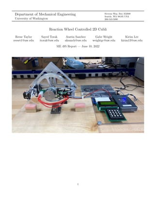
  • 1. Department of Mechanical Engineering University of Washington Stevens Way, Box 352600 Seattle, WA 98195 USA 206-543-5090 Reaction Wheel Controlled 2D Cubli Reese Taylor reeset1@uw.edu Sayed Torak itorak@uw.edu Austin Sanchez aksanch@uw.edu Gabe Weight weightgc@uw.edu Kirim Lee kirim13@uw.edu ME 495 Report — June 10, 2022 1
  • 2. Contents 1 Executive Summary 5 2 Introduction 5 2.1 Project Definition . . . . . . . . . . . . . . . 5 2.2 Functional Specifications . . . . . . . . . . . 5 2.3 Design approach . . . . . . . . . . . . . . . 6 3 Dynamic Model 6 3.1 Non-Linear Model . . . . . . . . . . . . . . 6 3.2 Linearized Model . . . . . . . . . . . . . . . 7 4 Control Overview 7 4.1 PI Controller . . . . . . . . . . . . . . . . . 8 4.2 Linear Quadratic Integral Controller . . . . 8 5 Simulation Design 8 5.1 Parameter Estimation . . . . . . . . . . . . 9 5.2 Linear vs Non-Linear Model . . . . . . . . . 9 5.3 Jump-up Modeling . . . . . . . . . . . . . . 9 5.4 Current Step Disturbance . . . . . . . . . . 10 5.5 Recovery Angle . . . . . . . . . . . . . . . . 10 6 Prototype Design 11 6.1 Purpose . . . . . . . . . . . . . . . . . . . . 11 6.2 Critical Component Selection . . . . . . . . 11 6.2.1 Motor . . . . . . . . . . . . . . . . . 11 6.2.2 Motor Controller . . . . . . . . . . . 12 6.2.3 Servo . . . . . . . . . . . . . . . . . 12 6.2.4 Collet Prop Adapter . . . . . . . . . 12 6.2.5 IMU . . . . . . . . . . . . . . . . . . 13 6.3 Mechanical Design . . . . . . . . . . . . . . 13 6.3.1 Frame and Motor Cantilever . . . . 13 6.3.2 Flywheel . . . . . . . . . . . . . . . 13 6.3.3 Braking System . . . . . . . . . . . . 14 6.3.4 CAD Model . . . . . . . . . . . . . . 14 6.3.5 Manufacturing . . . . . . . . . . . . 15 6.4 Electrical Design . . . . . . . . . . . . . . . 15 6.4.1 NI myRio-1900 . . . . . . . . . . . . 15 6.4.2 Power Supply . . . . . . . . . . . . . 15 6.4.3 Servo Battery . . . . . . . . . . . . . 15 6.4.4 Encoder . . . . . . . . . . . . . . . . 16 6.5 Computational Design . . . . . . . . . . . . 16 6.5.1 Complementary Filter . . . . . . . . 16 6.5.2 Finite State Machine . . . . . . . . . 17 6.5.3 Off State . . . . . . . . . . . . . . . 18 6.5.4 Speed Up State . . . . . . . . . . . . 18 6.5.5 Brake State . . . . . . . . . . . . . . 18 6.5.6 Brake to Balance State . . . . . . . 18 6.5.7 Balance State . . . . . . . . . . . . . 18 6.6 Final Assembly . . . . . . . . . . . . . . . . 18 7 Testing 18 7.1 IMU vs Encoder . . . . . . . . . . . . . . . 18 7.2 Current Disturbance Response . . . . . . . 19 7.3 Jump Up Response . . . . . . . . . . . . . . 19 7.4 Max Recovery Response . . . . . . . . . . . 20 7.5 Hall Sensor Issue . . . . . . . . . . . . . . . 20 7.6 Comparison to Functional Specifications . . 21 8 Risk and Liability 21 9 Ethical Issues 22 10 Impact on Society 22 11 Impact on the Environment 22 12 Cost and Engineering Economics 22 13 Codes and Standards 23 14 Conclusions 23 14.1 Continued development . . . . . . . . . . . 23 14.2 Final product configuration . . . . . . . . . 23 15 Appendix 25 15.A Simulink Block Diagrams . . . . . . . . . . 25 15.B Manufacturing Drawings . . . . . . . . . . . 29 15.C Wiring Diagram . . . . . . . . . . . . . . . 35 15.D Code . . . . . . . . . . . . . . . . . . . . . . 36 15.D.1 Main Thread Diagram . . . . . . . . 36 15.D.2 IRQ Timer Thread Diagram . . . . 37 15.E Component Specification Sheets . . . . . . . 38 15.E.1 Motor Specifications . . . . . . . . . 38 15.E.2 Motor Controller Specifications . . . 40 2
  • 3. List of Figures 1 Cubli Body Free Body Diagram . . . . . . . . . . . . . . . . . . . . . . . . . . . . . . . . . . . . . . . . . . 6 2 Cubli Wheel Free Body Diagram . . . . . . . . . . . . . . . . . . . . . . . . . . . . . . . . . . . . . . . . . 7 3 Nonlinear Cubli Plant Model . . . . . . . . . . . . . . . . . . . . . . . . . . . . . . . . . . . . . . . . . . . 7 4 PI Control Loop . . . . . . . . . . . . . . . . . . . . . . . . . . . . . . . . . . . . . . . . . . . . . . . . . . 8 5 LQI Control Loop . . . . . . . . . . . . . . . . . . . . . . . . . . . . . . . . . . . . . . . . . . . . . . . . . 8 6 Comparison of Linear and Nonlinear Systems . . . . . . . . . . . . . . . . . . . . . . . . . . . . . . . . . . 9 7 Simulated Jump Up Response . . . . . . . . . . . . . . . . . . . . . . . . . . . . . . . . . . . . . . . . . . . 9 8 Simulated current disturbance state variable response . . . . . . . . . . . . . . . . . . . . . . . . . . . . . 10 9 Simulated controller current response . . . . . . . . . . . . . . . . . . . . . . . . . . . . . . . . . . . . . . . 11 10 Simulated 2◦ recovery angle response . . . . . . . . . . . . . . . . . . . . . . . . . . . . . . . . . . . . . . . 11 11 Maxon EC 45 Flat 70W Brushless DC Motor . . . . . . . . . . . . . . . . . . . . . . . . . . . . . . . . . . 12 12 ESCON 36/3 EC Motor Controller . . . . . . . . . . . . . . . . . . . . . . . . . . . . . . . . . . . . . . . . 12 13 Reefs RC 99 Micro . . . . . . . . . . . . . . . . . . . . . . . . . . . . . . . . . . . . . . . . . . . . . . . . . 13 14 Collet Prop Adapter . . . . . . . . . . . . . . . . . . . . . . . . . . . . . . . . . . . . . . . . . . . . . . . . 13 15 SparkFun LSM9DS1 9DOF IMU . . . . . . . . . . . . . . . . . . . . . . . . . . . . . . . . . . . . . . . . . 13 16 Frame CAD Render . . . . . . . . . . . . . . . . . . . . . . . . . . . . . . . . . . . . . . . . . . . . . . . . 14 17 Flywheel CAD Render . . . . . . . . . . . . . . . . . . . . . . . . . . . . . . . . . . . . . . . . . . . . . . . 14 18 Braking System CAD Render - Back View . . . . . . . . . . . . . . . . . . . . . . . . . . . . . . . . . . . . 14 19 Braking System CAD Render - Front View . . . . . . . . . . . . . . . . . . . . . . . . . . . . . . . . . . . 14 20 Final Prototype CAD Render . . . . . . . . . . . . . . . . . . . . . . . . . . . . . . . . . . . . . . . . . . . 15 21 Final Prototype CAD Render - Top View . . . . . . . . . . . . . . . . . . . . . . . . . . . . . . . . . . . . 15 22 Reaction Wheel Manual CNC Manufacturing . . . . . . . . . . . . . . . . . . . . . . . . . . . . . . . . . . 15 23 NI myRio-1900 Embedded Computer . . . . . . . . . . . . . . . . . . . . . . . . . . . . . . . . . . . . . . . 16 24 24V Mean Well power supply with 12.5A output . . . . . . . . . . . . . . . . . . . . . . . . . . . . . . . . 16 25 6V 1600mAh RC Servo Battery . . . . . . . . . . . . . . . . . . . . . . . . . . . . . . . . . . . . . . . . . . 16 26 US Digital S2-2000-B Optical Quadrature Encoder . . . . . . . . . . . . . . . . . . . . . . . . . . . . . . . 16 27 Complementary Filter Block Diagram . . . . . . . . . . . . . . . . . . . . . . . . . . . . . . . . . . . . . . 16 28 Complementary Filter Bode Plot . . . . . . . . . . . . . . . . . . . . . . . . . . . . . . . . . . . . . . . . . 17 29 State Transition Diagram . . . . . . . . . . . . . . . . . . . . . . . . . . . . . . . . . . . . . . . . . . . . . 17 30 Final Assembly . . . . . . . . . . . . . . . . . . . . . . . . . . . . . . . . . . . . . . . . . . . . . . . . . . . 18 31 Encoder vs IMU response . . . . . . . . . . . . . . . . . . . . . . . . . . . . . . . . . . . . . . . . . . . . . 19 32 5A current disturbance state variable response . . . . . . . . . . . . . . . . . . . . . . . . . . . . . . . . . 19 33 Controller current response . . . . . . . . . . . . . . . . . . . . . . . . . . . . . . . . . . . . . . . . . . . . 19 34 Jump Up to Balancing Response . . . . . . . . . . . . . . . . . . . . . . . . . . . . . . . . . . . . . . . . . 20 35 Maximum Recovery Angle Response . . . . . . . . . . . . . . . . . . . . . . . . . . . . . . . . . . . . . . . 20 36 Hall Sensor Issue - Actual vs Measured Wheel Velocity . . . . . . . . . . . . . . . . . . . . . . . . . . . . . 21 37 Simulated jump up response using recorded wheel data . . . . . . . . . . . . . . . . . . . . . . . . . . . . . 21 38 Full Simulink Block Diagram . . . . . . . . . . . . . . . . . . . . . . . . . . . . . . . . . . . . . . . . . . . 25 39 Cubli Plant Simulink Model . . . . . . . . . . . . . . . . . . . . . . . . . . . . . . . . . . . . . . . . . . . . 26 40 Simulink Braking System . . . . . . . . . . . . . . . . . . . . . . . . . . . . . . . . . . . . . . . . . . . . . 27 41 Simulink PI Speed Controller . . . . . . . . . . . . . . . . . . . . . . . . . . . . . . . . . . . . . . . . . . . 27 42 Simulink LQI Balance Controller . . . . . . . . . . . . . . . . . . . . . . . . . . . . . . . . . . . . . . . . . 28 43 Frame Drawing File . . . . . . . . . . . . . . . . . . . . . . . . . . . . . . . . . . . . . . . . . . . . . . . . 29 44 Cantilever Base Drawing File . . . . . . . . . . . . . . . . . . . . . . . . . . . . . . . . . . . . . . . . . . . 30 45 Cantilever Motor Mount Drawing File . . . . . . . . . . . . . . . . . . . . . . . . . . . . . . . . . . . . . . 31 46 Flywheel Drawing File . . . . . . . . . . . . . . . . . . . . . . . . . . . . . . . . . . . . . . . . . . . . . . . 32 47 Caliper Drawing File . . . . . . . . . . . . . . . . . . . . . . . . . . . . . . . . . . . . . . . . . . . . . . . . 33 48 Servo Mount Drawing File . . . . . . . . . . . . . . . . . . . . . . . . . . . . . . . . . . . . . . . . . . . . . 34 49 Wiring Diagram . . . . . . . . . . . . . . . . . . . . . . . . . . . . . . . . . . . . . . . . . . . . . . . . . . 35 50 Main Thread Flowchart . . . . . . . . . . . . . . . . . . . . . . . . . . . . . . . . . . . . . . . . . . . . . . 36 51 Timer IRQ Thread Flowchart . . . . . . . . . . . . . . . . . . . . . . . . . . . . . . . . . . . . . . . . . . . 37 3
  • 4. List of Tables 1 Functional Specifications . . . . . . . . . . . . . . . . . . . . . . . . . . . . . . . . . . . . . . . . . . . . . . 6 2 List of Symbols . . . . . . . . . . . . . . . . . . . . . . . . . . . . . . . . . . . . . . . . . . . . . . . . . . . 6 3 List of Parameters . . . . . . . . . . . . . . . . . . . . . . . . . . . . . . . . . . . . . . . . . . . . . . . . . 9 4 EC 45 Flat 70W specifications . . . . . . . . . . . . . . . . . . . . . . . . . . . . . . . . . . . . . . . . . . 12 5 ESCON 36/3 EC Specifications . . . . . . . . . . . . . . . . . . . . . . . . . . . . . . . . . . . . . . . . . . 12 6 Reefs RC 99 Micro Specifications . . . . . . . . . . . . . . . . . . . . . . . . . . . . . . . . . . . . . . . . . 12 7 Comparison to Functional Specifications . . . . . . . . . . . . . . . . . . . . . . . . . . . . . . . . . . . . . 21 8 Purchase list . . . . . . . . . . . . . . . . . . . . . . . . . . . . . . . . . . . . . . . . . . . . . . . . . . . . 23 4
  • 5. 1 Executive Summary The three-dimensional Cubli is a reaction wheel con- trolled inverted pendulum system that is capable of balanc- ing itself on an edge or corner as well as jumping itself up to a balance position from flat on a table. This report de- scribes the design process, dynamic modeling, simulation, physical implementation, testing, and results of building a two-dimension prototype of the full Cubli system. It com- pares the results of simulation predictions to that of the physical prototype for several distinct testing procedures, justifies the differences, and discusses areas of improvement for future iterations. A mathematical model of the two-dimensional Cubli dy- namic system was derived from basic equations of motion and physics relationships, and two different linear con- trollers were developed to control the speed of the fly- wheel and to balance the system about a corner based on this model. The controllers were designed to meet the functional specifications outlined at the start of the project. The model and controllers were then simulated using Simulink and a MATLAB script to predict the be- havior of the system during a jump up process, a current disturbance, and an angle initial condition response. Several components of the prototype were manufactured in the ME machine shop out of available aluminum stock material. These components included the frame, flywheel, braking system, and motor cantilever mounts, all of which were designed in Solidworks to maximize strength and min- imize weight, while providing robust connections between critical components. State estimation and feedback was accomplished via a Sparkfun 9Dof Inertial Measurement Unit (IMU) to mea- sure the angle and angular velocity of the cubli body, and Hall sensors built into the flywheel motor to measure the angular velocity of the wheel. The use of an IMU over an encoder for angle measurements allowed the system to stay balanced while the orientation of the supporting base is changed. A complementary filter was implemented to pro- vide a more accurate estimation of the angle of the body by combining data from both the accelerometers and gy- roscopes. The computational control and data collection for the system were accomplished using a program built in C run- ning on a myRIO-1900 embedded computer. This com- puter communicates with the Cubli prototype to estimate the current state via the IMU and Hall sensors, provide current to the motor to speed up the flywheel, and con- trol the orientation of an RC servo to actuate the braking system. The Maxon EC 45 Flat 70W Brushless DC motor was controlled using an ESCON 36/3 EC 4-quadrant mo- tor controller that received analog set values for the desired motor current from the myRIO-1900. The RC servo motor orientation was controlled by adjusting the duty cycle of a Pulse Width Modulated (PWM) signal sent to the servo motor via the myRIO-1900. The C program integrates this state estimation with a fi- nite state machine to control the current sent to the Cubli prototype and the transition between five distinct states including an off state, a speed up state, a brake state, a brake to balance state, and a balancing state. The state machine relies on a separate Timer IRQ thread for timing with a sample rate of 5ms, and the transitions are con- trolled by conditions related to the current state variables, keypad button presses, and timing variables. A final prototype was assembled and several tests were conducted to compare the simulated dynamic behavior to the real world behavior. These tests included jump up to balance tests, a 5A forced current disturbance test, and a maximum recovery angle test, all of which showed close agreement between the simulated and real results. Fur- ther analysis was presented to quantify the difference be- tween the simulation predictions and actual results, and limiting issues were identified and discussed. Final conclu- sions were presented that consider the overall success of the project and recommended directions in which future iterations should proceed. 2 Introduction 2.1 Project Definition The Cubli is a reaction wheel controlled inverted pendu- lum system in the shape of a cube and was first developed by The Institute for Dynamic Systems and Control at ETH Zurich university [1]. The system is capable of transferring momentum stored in the three actively controlled onboard flywheels to the external frame via a mechanical braking system, allowing it to jump up from a face onto an edge or corner and actively balance while rejecting disturbances. The goal of this capstone project is to design and develop a functioning two-dimensional prototype of the full three- dimensional Cubli with only one rotational degree of free- dom. This prototype will be able to jump up from its edge to a corner and actively balance in an unstable position by applying torque to the system’s flywheel. The design will include a mechanical braking system, a PI speed controller to initiate the momentum transferring jump up procedure, and an LQI state feedback controller to actively balance the system on a corner. 2.2 Functional Specifications To aid in a successful project, the following quantitative functional specifications were set as target goals for the final prototype. 5
  • 6. Table 1: Functional Specifications Jump up success rate >95 % Maximum recovery angle >7◦ Total mass <1 kg Recovery overshoot <75 % Recovery settling time <3 s Steady state error <1◦ 2.3 Design approach The main considerations for the prototype design were scope and performance. Firstly, the scope of this project was limited to a two-dimensional Cubli system to allow for full completion within the two quarter timeline. This led to prioritizing simplicity where possible, such as in the braking system and flywheel design. With additional time and resources, the final prototype presented in this report can be easily extrapolated to build a full three-dimensional Cubli system without much additional effort, since the de- sign and control for a single rotational degree of freedom has already been achieved. Secondly, the prototype was designed to meet or exceed the functional specifications listed above. One key consid- eration to accomplish this was the sizing of the system and the various components used. The mass of the system was limited to less than one kilogram as to require less angular velocity and torque from the motor to effectively jump up to the corner and correct for disturbances. So the system was sized accordingly to accomplish this. Furthermore, re- liability was a major consideration while developing the final prototype. A jump up success rate greater than 95% was desired, so the design for the final prototype was based mainly on minimizing weight and maximizing reliability. 3 Dynamic Model 3.1 Non-Linear Model The dynamic model of the cubli is based on the deriva- tions presented in [2] and [3]. The equations of motion for the system are derived from the free body diagrams of the cubli body and flywheel shown in Figures 1 and 2 re- spectively, and the parameters used in this derivation are summarized in Table 2. The flywheel is supported directly by the cubli body, which can rotate independently of the flywheel, so it is necessary to specify the angle of the wheel with respect to the angle of the body for this derivation, as shown in Figure 2. The cubli body is subjected to external torques from gravity and the motor as well as damping torques from the motor and pivot bearings. In the reference frame of the Table 2: List of Symbols Symbol Definition Units θb Body angle rad θ̇b Body angular velocity rad s θ̈b Body angular acceleration rad s2 θ̇w Wheel angular velocity rad s θ̈w Wheel angular acceleration rad s2 Bb Body damping N·m·s rad Bw Wheel damping N·m·s rad mb Body mass kg mw Wheel mass kg lw Pivot to wheel center m lb Pivot to center of mass m τm Motor torque N · m Iw Wheel inertia kg · m2 Ib Body inertia kg · m2 KKm Motor Constant Nm A cubli body, the flywheel is subjected to equal and opposite bearing and motor torques as well as an external force of gravity that causes a torque on the body. Figure 1: Cubli Body Free Body Diagram The equation of motion for the cubli body is summarized in (1). Rewriting the torque terms in this equation to be in terms of the body angle, body angular velocity, and wheel angular velocity yields an expression for the angular acceleration of the body, shown in (2). 6
  • 7. Figure 2: Cubli Wheel Free Body Diagram (Ib + mwlw 2 )θ̈b = τBb + τg + τBw − τm (1) θ̈b = −Bbθ̇b + (mblb + mwlw)g · sin(θb) + Bwθ̇w − τm Ib + mwlw 2 (2) The equation for the angular acceleration of the flywheel is shown in (3), which directly depends on the angular acceleration of the cubli body due to the flywheel angle dependency on the angle of the body. From (2) and (3), the nonlinear block diagram of the cubli body is derived and shown in Figure 3. This model is set up as a single input multiple output system, since our strategy to control this system during balancing is based on the principles of full state control, thus requiring all state variables of the system as outputs. θ̈w = τm − Bwθ̇w − ¨ θb Iw (3) 3.2 Linearized Model Next, the nonlinear cubli plant model can be linearized about the operating point of θb = 0 using a small angle approximation so that sin(θb) ≈ θb. This removes the sin term from the plant model and allows for the derivation of a state space representation of our model in the form shown in (4) that is used in designing the balancing controller. Here the state vector of this system, x, is composed the angle of the cubli body, θb, the angular velocity of the body, θ̇b, and the angular velocity of the flywheel, θ̇w. The single Figure 3: Nonlinear Cubli Plant Model input to this system, u, is the current delivered to the motor. These expressions are summarized in (5). Finally, the A and B matrices are derived from the cubli plant model and shown in (6) and (7). ẋ = Ax + Bu, y = x (4) x =      θb θ̇b θ̇w      , u = h im i (5) A =       0 1 0 (mblb+mwlw)g Ib+mwlw 2 − Bb Ib+mwlw 2 Bw Ib+mwlw 2 −(mblb+mwlw)g Ib+mwlw 2 Bb Ib+mwlw 2 − Bw(Ib+Iw+mwlw 2 ) Iw(Ib+mwlw 2)       (6) B =       0 − Km Ib+mwlw 2 Km(Ib+Iw+mwlw 2 ) Iw(Ib+mwlw 2)       (7) 4 Control Overview Two separate controllers were used to control the Cubli prototype. A proportional-integral (PI) controller was de- veloped to control the angular velocity of the flywheel to a desired speed prior to braking. A linear quadratic integral controller (LQI) was developed to control all three state variables of the system simultaneously to achieve robust balancing performance. For both controllers, the output of the controller is a current sent directly to the motor 7
  • 8. controller operating in current controller mode. This al- lows for direct control of the torque applied to the motor in both cases. 4.1 PI Controller Figure 4: PI Control Loop The control loop for the PI speed controller is shown above in Figure 4. Here, the controller is only controlling the angular velocity of the flywheel, θ̇w, and not the other state variables. This controller is the same controller used in Lab 7 of ME 477 at the University of Washington, which is used to control the speed of a DC motor and inertial load. It is based on the continuous PI controller transfer function shown in the left box of Figure 4. This continuous controller transfer function was discretized using Tustin’s method and implemented with a linear difference equation using the function cascade() in the C control code. The final values of the proportional gain and integral gain terms in this transfer function are Kp = 0.25 Ki = 0.125. These were selected through iteration to achieve a fast speed up from 0 RPM to the desired angular ve- locity with minimal overshoot. To further minimize the overshoot of the speed up process, the function sramps() was implemented to create an angular velocity trajectory as the reference input, rather than a large step change. 4.2 Linear Quadratic Integral Controller Figure 5: LQI Control Loop The control loop for the Linear Quadratic Integral (LQI) feedback controller is shown above in Figure 5. This type of controller is similar to a linear quadratic regulator (LQR) that minimizes a cost function J to find the optimal gain matrix, K, given a set of system and power costs. The key difference between these control types is that the LQI con- troller augments the original state space representation of the Cubli system with an additional state z = R t 0 (r−y)dτ, representing the integral of the error signal for the wheel angular velocity, θw. This helps to drive the steady state error of the system to zero if there are errors between the dynamic model and real prototype parameters. The result- ing augmented state space model is shown below in equa- tion 8, where C = [ 0, 0, 1 ]. This type of controller was selected because of its ease of use and implementation and suitability for controlling a system in state space form. ẋ ż = A 0 −C 0 x z + B 0 u + 0 I r (8) Parameters such as performance (e.g. how quickly re- sponse returns to desired state) and effort (e.g. actuation effort) are optimized by the user defined matrices Q and R. These cost matrices were first selected using Bryson’s rule, where (xi)max and (ui)max are the largest reasonable input magnitudes for each state and input variable respec- tively, arranged along the diagonal of each matrix raised to the power of negative 2. These values were then tuned iteratively to achieve the best balancing performance, and the final cost matrices used are shown in 9 and 10. Q =       (1)−2 0 0 0 0 (5)−2 0 0 0 0 (2.7)−2 0 0 0 0 (15)−2       (9) R = (0.92)−2 (10) The lqi() function in MATLAB was then used to cal- culate the optimal gain matrix, K, by minimizing the quadratic cost function J in (11) with the defined cost ma- trices Q and R. This gain matrix can be represented by K = [ Kp, Ki ], where the Kp terms represent the LQR gain matrix, and the Ki term represents the gain for the integral state. The optimal gain matrix used in the final prototype is shown in 12. The controller was then imple- mented into the C control code following the control loop in Figure 5. J = Z ∞ 0 ( h xT zT i Q x z # + uT Ru dt (11) K = −144.4222 −19.8352 −0.3611 0.0613 (12) 5 Simulation Design A Simulink model in conjunction with a MATLAB script was developed to predict the dynamic performance of the system and speed/balance controllers used in the final pro- totype. The Simulink model is composed of the Cubli plant 8
  • 9. model shown in Figure 3, along with a LQI balance con- troller, PI speed controller, braking system, and logic to control the transitions between initiating the momentum transfer for the jump up and the balancing control. De- tailed images of these various block diagrams can be found in Figures 38 - 42 in Appendix A. 5.1 Parameter Estimation The parameters used in the Simulink model and MAT- LAB script were based on the actual parameters of the final prototype, which were determined in two ways. Firstly, the mass of the body, mb, and the mass of the wheel, mw, were measured directly after full prototype assembly, along with the length from the pivot to the center of the wheel, lw. Since precision bearings were used for both the body and wheel, the respective damping coefficients were very small and assumed to be zero. The remaining parameters were based on Solidworks inertia analysis on the final updated CAD model after adjusting the masses to match what was measured directly. The resulting parameters are shown in Table 3 below, which were used in all simulation results presented in this report. Table 3: List of Parameters Symbol Value Units mw 0.2201 kg lw 0.0955 m Iw 7.221 × 10⁻⁴ kg · m2 Bw 0 N·m·s rad mb 0.6123 kg lb 0.0934 m Ib 0.0119 kg · m2 Bb 0 N·m·s rad 5.2 Linear vs Non-Linear Model Figure 6 presents a simulated comparison between the non-linear dynamic model and linearized state space model for an initial condition response of θb = 5◦ . This response has no external torque input from the motor, so the re- sponse is expected to be unstable about θb = 0◦ and stable about θb = 180◦ , which is the exact behavior predicted by the simulation. Comparing the nonlinear initial condition simulation to the linearized approximation reveals that the linear ap- proximation for all state variables is extremely close to the nonlinear behavior up to an angle of θb ≈ 45◦ at t ≈ 0.3 sec. This indicates that the body angle range where the linear model closely approximates the non-linear model is much larger than the target control range for the LQI con- troller. The full range of motion of the final prototype is limited to ±45◦ , and the LQI is only intended to operate over a portion of this range, so the performance of the lin- earized LQI controller should not be severely affected by deviation from the target angle of 0◦ . Figure 6: Comparison of Linear and Nonlinear Systems 5.3 Jump-up Modeling Figure 7: Simulated Jump Up Response The jump-up procedure for the two-dimensional Cubli 9
  • 10. is achieved by increasing the velocity of the flywheel to a specified angular speed and rapidly braking the wheel along the outer edge. The braking mechanism is fixed to the body so that upon initiation of the braking, the mo- mentum of the wheel is transferred to the body via the friction force between the brake pads and the wheel sur- face. The Simulink model for the braking system is split into two sections. The first section simulates a supporting force on the body while the system is stationary. In real life, the body would be resting on a table surface prior to initiating the jump up procedure, which limits the body angle to ± 45◦ and prevents the body from moving as the wheel ac- celerates. This behavior is not captured by the differential equations, so to model this, all active accelerations signals were identified and fed back into the system as negative signals. This allows the simulation to accelerate the fly- wheel to the desired speed while maintaining the angle of the body at 45◦ . The next section in the braking model is used to slow down the wheel and transfer momentum to the body. This is achieved by introducing equal and opposite external torques to the body and wheel that represent the torque applied to the wheel and body by a mechanical braking system. To apply the torques appropriately, a group of logic operators were implemented to the Simulink model that check if enough momentum is transferred to the body to lift it off the table. The logic operators then turn off all table support signals and keep the momentum transfer signal active. Once the angle of the body reaches a speci- fied angle, the LQI controller is activated and the system is balanced. This Simulink model was used to accurately compute the minimum angular velocity of the flywheel required for some specified final jump-up angle based on an approx- imate impulse in the braking force applied to the wheel. The approximate impulse function was applied using a step pulse with an extremely small width and large amplitude, to simulate the conditions of a perfect impulse. The model developed was compared against theoretical speeds that were calculated using (13), which is derived from a per- fectly inelastic momentum transfer between the wheel and body [3]. ω2 w = (2 − √ 2) Iw + Ib + mwl2 w I2 w (mblb + mwlw) ge (13) Equation 12 predicts a wheel velocity of θ̇w = -1073.6 RPM to bring the body from an initial angle of 45◦ ex- actly to 0◦ . Our simulation results predict θ̇w ≈ -1090 RPM to bring the body angle from an initial angle of 45◦ to nearly 0◦ , which is extremely close to that of the perfect momentum transfer as well as the actual jump up speed selected for the final prototype of -1080 RPM. The sim- ulation plots of the state variable jump up and balance response are shown in Figure 7. 5.4 Current Step Disturbance Figure 8: Simulated current disturbance state variable re- sponse Figures 8 and 9 presents a simulated current disturbance response. In this, an external current disturbance of 5A is added to the LQI controller current output that is sent to the non-linear Cubli plant model. The simulation then predicts the state variable responses to this current dis- turbance as well as the controller current output, current sent to the motor, and resulting motor torque. Note that the controller current output settles at a value of -5A to exactly cancel with the 5A disturbance, resulting in zero current and zero torque sent to the motor in steady state. 5.5 Recovery Angle Figure 10 shows a simulated 2◦ recovery angle balancing response for each state variable. In this, the initial body angle was set to θb = 2◦ , and the initial body and wheel velocities were set to zero. This imitates the LQI controller response to a 2◦ step change in the reference angle. 10
  • 11. Figure 9: Simulated controller current response Figure 10: Simulated 2◦ recovery angle response 6 Prototype Design 6.1 Purpose The main purpose of this prototype was to compare the simulation predictions with a real life prototype to verify both the simulation results and final design. Additionally, the purpose of this prototype was to explore and imple- ment mechatronics concepts in a hands-on context. Creat- ing a physical prototype presented challenges in manufac- turing, assembly, and moving from theoretical concepts to their practical application. This prototype was an oppor- tunity to move beyond the classroom and gain real-world engineering experience. Furthermore, this prototype also served as a proof-of- concept and starting point for development of a full 3D Cubli prototype. The scope of a fully 3D Cubli prototype from scratch is too large to complete in two quarters, so this prototype can be viewed directly as a starting point for developing the full Cubli system. 6.2 Critical Component Selection The final prototype has several critical components that are necessary for proper operation of the two-dimensional Cubli. These include the motor, motor controller, RC servo motor, collet propeller adapter, and inertia measure- ment unit. More detail is provided for each of these com- ponents in the following sections. A useful method used in selecting these final components was examining the choices made by other Cubli projects. Several papers that included detailed lists of which parts were used and why they were selected [1][4][5][2][6], which provided valuable resources to draw ideas from initially. The search was then narrowed to fit the desired functional specifications and ensure compatibility between compo- nents. 6.2.1 Motor The motor for the final prototype is the Maxon EC 45 Flat 70W Brushless DC motor. This motor has built in Hall sensors for commutation and measurement of angular velocity directly, which was a critical aspect for the feed- back control system. An image of the motor and some important specifications are shown below in Figure 11 and Table 4. One difficulty confronted during motor selection is the trade-off between torque and angular velocity. Motors that are geared to have high output torque have low operating speeds and those meant to operate at high speed have low torque output. Further complicating the choice was the need to keep the mass and volume as low as possible for each component. The EC 45 Flat 70W motor has a good combination of high torque and high speeds while minimiz- ing weight, so it was an ideal choice to control the flywheel without adding unnecessary mass or requiring excessive power consumption. 11
  • 12. Figure 11: Maxon EC 45 Flat 70W Brushless DC Motor Table 4: EC 45 Flat 70W specifications Parameter Spec Units Nominal Voltage 24 V Nominal speed 4860 rpm Nominal torque 128 mN · m Nominal Current 3.21 A Stall torque 1460 mN · m Torque constant 36.9 mN·m A Speed constant 259 rpm V Mass 141 g Figure 12: ESCON 36/3 EC Motor Controller 6.2.2 Motor Controller The compatible controller to control this motor was the ESCON 36/3 EC 4-quadrant servo controller sourced from Maxon as seen in Figure 12. The driver input for the ES- CON 36/3 EC is an analog voltage input that controls the set value of either the current or desired speed depend- ing on the operating mode, and a digital enable signal to turn the controller on and off. The motor controller can be used as both a speed and current controller with real time monitoring of the actual speed and current values as analog outputs, and comes with a very easy to use setup software making it the optimal choice for this project and motor. The important specifications are listed in Table 5. Table 5: ESCON 36/3 EC Specifications Parameter Spec Unit Nominal Voltage 10 - 36 V Maximum Output Voltage 38.0 V Continuous Output Current 2.7 A Maximum Output Current 9.0 A Weight 36.0 g PWM Frequency 53.6 kHz 6.2.3 Servo The braking system for the final prototype is actuated via the Reefs RC 99 Micro servo motor, which can be seen in Figure 3. The critical characteristic of this servo mo- tor is its very high stall torque and relatively low weight. The rate at which this motor can slow down the flywheel is directly related to the torque provided by the servo mo- tor, so high torque was necessary to ensure reliability. The weight of the Reefs RC 99 Micro was one of the lightest op- tions considered weighing at ≈20 grams. Several additional specifications can be seen detailed in Table 6. The angular position of the servo rotor is controlled by adjusting the duty cycle of a pulse width modulated (PWM) signal sent directly to the motor from the embedded computer. Table 6: Reefs RC 99 Micro Specifications Parameter @ 6.0 V @ 7.4 V @ 8.4 V Unit Nominal Speed 0.110 0.090 0.080 s Nominal Torque 89 99 115 oz · in Stall Current 2.0 2.2 2.4 A 6.2.4 Collet Prop Adapter A challenging aspect of the final prototype design was the connection between the motor shaft and the manufac- tured flywheel. The final solution involves the addition of a propeller collet adapter that simultaneously attaches the motor, flywheel, and frame together. This attachment method was selected so that the concentricity of the mo- tor shaft aligns with the internal diameter of the flywheel, 12
  • 13. Figure 13: Reefs RC 99 Micro and so that the forces holding the flywheel on the adapter also clamp the collect onto the motor shaft, providing a ro- bust means of connection. An image of the collet adapter can be seen in Figure 14. The internal diameter of the collet adapter used was slightly larger than the diameter of the motor shaft, so a 1mm thick brass sleeve was in- serted between these components to ensure a tight, highly concentric fit. Figure 14: Collet Prop Adapter 6.2.5 IMU The final Cubli prototype used a SparkFun 9DoF Stick which is a 9 degree of freedom, 0.9”x0.4” IMU that utilizes a LSM9DS1 sensor with an I2C bus. The LSM9DS1 sensor has 3 accelerometers, 3 gyroscopes, and 3 magnetometers which measure 3 degrees of each proper acceleration, an- gular velocity, and magnetic orientation relative to Earth’s magnetic field, respectively. The IMU was mounted onto the frame so that its positive x- and y-axis matched the prototype’s coordinate system. The main reason for using an IMU over an encoder to measure the angle and velocity of the body is to allow the Cubli system to remain balanced regardless of the orienta- tion of the base. With an encoder mounted to the base, the 0◦ desired balance orientation always remains perpendicu- lar to the base. The direction of gravity does not change, so the controller will be unable to balance the system if the angle of the base changes because of this. However, by using an IMU, the 0◦ desired balance orientation is defined with respect to the direction gravity, so adjusting the base angle will have no effect on the system’s ability to balance, which is desirable. Figure 15: SparkFun LSM9DS1 9DOF IMU 6.3 Mechanical Design 6.3.1 Frame and Motor Cantilever The frame was designed with considerations made to minimize mass while ensuring compatible integration be- tween the others parts in the final prototype such as the braking assembly, collet adapter shaft, IMU, and pivot at- tachment. A CAD render of the final design is shown in Figure 16. Additionally, two components that comprise a cantilever attached to the frame were design to hold the motor and motor controller securely to the frame without interfering with the motion of the flywheel. 6.3.2 Flywheel The main factors in designing the flywheel were the bi- axial forces on the motor shaft, weight restrictions, com- patibility with the prop adapter, and enough space for the brakes. The final design shown in Figure 17 accounts for each of these factors and includes high tolerances to mini- mize forces on the motor shaft. Given the maximum radial load on the motor shaft acquired from the specification sheet, the tolerance for the wheel was calculated using ba- sic centrifugal force mechanics based on a range of expected wheel speeds. The maximum eccentricity allowed in the design that would result in a radial force half that of the maximum allowable was determined, which corresponds to a factor of safety of 2. The final product is highly accu- rate and well balanced, minimizing any potential damage 13
  • 14. Figure 16: Frame CAD Render to the critical components. Figure 17: Flywheel CAD Render 6.3.3 Braking System Figures 18 and 19 show CAD renders of the final proto- type braking system. This system functions very similarly to sliding caliper braking mechanisms found commonly on cars. The RC servo motor is mounted to the top of the sys- tem via a servo mounting structure attached to the main brake caliper. Actuation of the servo motor turns a plas- tic servo horn extension against a cylindrical Delrin cam, depressing a spring loaded shoulder bolt attached directly to a bicycle brake pad. When this upper brake pad makes contact with the wheel, additional torque provided by the RC servo contributes to lifting the entire caliper assembly off the frame, bringing the bottom brake pad into con- tact with the other side of the flywheel. Additional spring loaded shoulder bolts on the back of the brake caliper aid in releasing the brake pads from the wheel when the servo is disengaged, and also serve to attach the entire braking Figure 18: Braking System CAD Render - Back View system to the frame. Figure 19: Braking System CAD Render - Front View The full mechanism was designed to be lightweight yet sturdy enough to handle the high torque applied by the servo motor. Other considerations were made such as the stiffness of the springs, material of the cylindrical cam, and brake pad material during the designing of this system to facilitate strong and reliable engagement and release of the brake pads from the servo. 6.3.4 CAD Model The final prototype CAD renders are shown in Figures 20 and 21. These photos call out the various mechanical 14
  • 15. and electrical components used in the final prototype and show the final assembly configuration. Figure 20: Final Prototype CAD Render Figure 21: Final Prototype CAD Render - Top View 6.3.5 Manufacturing All structural components, including the flywheel, frame, brake caliper/servo mount, and cantilever motor mount were manufactured out of Aluminum stock mate- rial in the ME machine shop using the manual mills, lathes, and the water jet. The remaining components were either externally sourced or acquired through Professor Garbini, Bill Kuykendall, and on campus engineering clubs. Figure 22 shows the reaction wheel being manufactured at the on campus Machine Shop with the manual 2-axis CNC. De- tailed manufacturing drawings can be found in Figures 43 - 48 in Appendix B. 6.4 Electrical Design The following sections outline the major electrical com- ponents of the final prototype other than those already dis- Figure 22: Reaction Wheel Manual CNC Manufacturing cussed. A detailed electrical schematic including all elec- tric connections can be found in Figure 49 in Appendix C. 6.4.1 NI myRio-1900 The embedded computer used for the final prototype is the National Instruments myRIO-1900 embedded com- puter. This is the same computer used for all labs in ME 477, which allowed for easy modification of code developed in that class for this project. The myRIO is used along with a LCD display and numerical keypad connected to connector B. The IMU signals and RC servo PWM signal are connected to connector A, and the AIO of the motor controller is connected to connector C in the final proto- type. 6.4.2 Power Supply The power supply used for the final prototype is the Mean Well SPV-300-24 switching power supply. It pro- vides 24V and up to 12.5A of current output directly to the motor controller, which is higher than the maximum allowable current into the motor controller meaning there is more power available than needed. An image of this power supply is shown in Figure 24. 6.4.3 Servo Battery The power supply chosen to power the RC servo is a 6V, 1600mAh capacity NiMH servo battery made by Dy- namite. The battery provides up to 2A of current output when the servo motor is stalled during braking. This bat- 15
  • 16. Figure 23: NI myRio-1900 Embedded Computer Figure 24: 24V Mean Well power supply with 12.5A output tery is connected directly to the RC servo, and the negative terminal is grounded to the DGND pin of connector A on the myRIO-1900. An external charging station is used to recharge the battery after sustained operation. The servo battery used can be seen in Figure 25. Figure 25: 6V 1600mAh RC Servo Battery 6.4.4 Encoder The encoder used in the final prototype to directly mea- sure the angle and speed of the body is the US Digital S2-2000-B Optical Quadrature Encoder. The encoder is only used in the final design to verify the angles and speeds measured by the IMU are accurate to the encoder values after filtering. The complementary filter break frequency was determined using this encoder, which will be discussed in more detail in the Computational design section below. The encoder is connected directly to connector C on the myRIO-1900 via a Quanser terminal board. Figure 26: US Digital S2-2000-B Optical Quadrature En- coder 6.5 Computational Design 6.5.1 Complementary Filter Figure 27: Complementary Filter Block Diagram A complementary filter was implemented to filter the raw IMU angle and velocity measurements, providing a wider frequency range of valid angle measurements.The built in accelerometers of the IMU are used to measure the direction of the gravity vector, allowing for calculation of the angular orientation of the body. However, rapid 16
  • 17. accelerations and velocities can introduce error in the di- rection the measured acceleration vector points, skewing the angle results making the accelerometer readings valid only at low frequencies of motion over longer periods of time. The built in rate gyroscopes differ from the accelerome- ters in that they measure the angular velocity of the body directly. This velocity can then be integrated to obtain the angle of the body, which can result in drift in the an- gle over time due to the constant integration, making them only useful at higher frequencies of operation over shorter periods of time. So, the complementary filter combines both the accelerometers and gyroscopes together to filter out the high frequency effects on the accelerometer and low frequency effects on the gyroscopes with a low pass and high pass filter respectively, resulting in clean mea- surements of the body angle over a wider frequency range. A block diagram of the parallel filter combination is shown in Figure 27. Much of the work that goes into creating a complemen- tary filter is in the selection of the filter break frequency. The filters for the two sensors are chosen to have the same break frequency so that the parallel combination of filters has a unity magnitude over all frequencies, as shown in Figure 28. The final break frequency of 1.2566 rad/s was chosen through trial and error with constant examination of how the complementary filtered body angle compared to the body angle measured directly from the encoder. The results of these tests are shown in the Testing section be- low. Both the low pass and high pass filters for this com- plementary filter were discretized using Tustin’s method, converted to a series of second order biquad systems, and implemented in the main C control code using the func- tion cascade() to compute the next value using a linear difference equation. 6.5.2 Finite State Machine To implement the sequence from our prototype’s jump up state, braking state, to the eventual act of balancing the Cubli on its edge, a finite state machine was imple- mented to the C control code utilizing a timer IRQ thread with a 5 ms sample time. Each time through the IRQ assertion loop, the current state variables are measured, and then the current state function is called. The state transitions between each of the five states are triggered by various inputs including the current measurements of the body angle, body velocity, and wheel velocity, button presses on the keypad, and builtin timer variables. These transitions handle the entire functionality of speeding up the flywheel using the PI controller, applying the brake by adjusting the PWM duty cycle, and then balancing the cubli with the LQI controller. Prior to starting the state machine, all necesary initialization for the AIO, DIO, IMU, Figure 28: Complementary Filter Bode Plot Off Speed Up Brake Balance Timer 800 | (|Wheel_Vel| - |Jump_speed|) | 2.42 Timer = 0 Speed_up_on = 0 Speed_up_on != 0 |Wheel_Vel| 5 |Frame_Vel| 5   Go_to_off = 0 PWM Duty Cycle = 63% Timer = 0 Motor Controller = Enabled PI Controller = Enabled Timer 6000 || Go_to_off != 0 Speed_up_on = 0 Timer = 0 Motor Controller = Disabled PI Controller = Disabled PI Controller = Disabled PWM Duty Cycle = 63.5% Brake to Balance Go_to_off != 0 || Frame_Angle -30 || Frame_Angle 30 Speed_up_on = 0 Motor Controller = Disabled LQI Controller = Disabled -2 Frame_Angle 2 LQI Controller = Enabled PWM Duty Cycle = 60% Timer 500 |Frame_Vel| 5 PWM Duty Cycle = 60% Timer = 0 Figure 29: State Transition Diagram and PWM signals is completed. All the corresponding in- put conditions and resulting outputs are discussed in the following sections, and the full transition diagram can be seen in Figure 29. The full C control code along with flow charts for the main and Timer IRQ threads can be found in Appendix D. 17
  • 18. 6.5.3 Off State In this state, the Cubli system is stationary and at rest with no current sent to the flywheel. This state was imple- mented as a baseline state from which to initiate the jump up and balancing procedures as well as a safety check if the jump up or balancing process fails. All states except the brake state can transition to the off state, but the off state can only transition to the speed up state if the sys- tem is motionless and a button is pressed on the keypad to initiate the speed up of the flywheel. 6.5.4 Speed Up State In this state, the flywheel is accelerated along a refer- ence velocity profile generated by the function sramps() using the PI speed controller until it reaches a target jump up velocity. This state will then hold this velocity for a few seconds before transitioning to the Brake state. If a problem occurs or the speed of the wheel does not reach the target velocity, it will transition back to the off state. 6.5.5 Brake State In this state, the PI speed controller is disabled and the PWM signal sent to the RC servo motor is adjusted to en- gage the braking system. It then immediately transitions to the brake to balance state. 6.5.6 Brake to Balance State This state handles the transition from the brake state to the fully balancing state. When the target angle to start balancing is reached, this state will release the brake and activate the LQI balance controller before transitioning to the balancing state. If the target angle is not reached, it will transition back to the off state. 6.5.7 Balance State This is the final state in which the cubli remains bal- anced from the active LQI balancing controller. The sys- tem will remain balancing in this state as long as the angle of the body stays within ±30◦ . If this condition is broken or a button on the keypad is pressed to move to the off state, it will transition directly to the off state. 6.6 Final Assembly Figure 6.6 shows the final assembly of our prototype in its balancing state, including all mechanical and electric components. Figure 30: Final Assembly 7 Testing 7.1 IMU vs Encoder Provided the break frequency of 1.2566 rad/sec, the fol- lowing graphs as shown in Figure 31 were examined to compare the encoder to the IMU’s reading of the frame angle and the encoder to the gyroscope’s reading for the frame’s angular velocity. From this, it can be seen that the comparative data almost perfectly overlaps with one another under both slow and rapid movement, indicating the selected break frequency results in highly accurate an- gle measurements from the IMU. This helped justify the decision of the final chosen break frequency as well as the full transition to using the IMU over the encoder for angle and velocity measurements of the body. 18
  • 19. Figure 31: Encoder vs IMU response 7.2 Current Disturbance Response A current disturbance of 5A was sent to the motor to test the disturbance response of the system. The main goals of this test were to measure the response of the LQI controller during re-balancing of the system and to see how well the simulated disturbance response matches with the actual motion of the system. This is shown in Figure 32 where the simulated and actual frame angle, frame velocity, and wheel velocity are plotted. For the simulation, a 5 A step in current was simply added onto the input current to the motor via a Sum block. Figure 33 shows the response from the controller due to the disturbance. In all these cases, the simulated re- sponse and actual response match very well omitting the noise generated by the sensors, indicating the simulation is a good model of the physical system. The simulated angle of the frame vs the actual angle of the frame during the disturbance has higher error than the other plots, but this can be attributed mostly to a non-zero balancing position of the physical system. The center of mass location as well as the orientation of the wires on the back of the proto- type contribute to slight deviations in the angle at which the system is fully balanced, so the real system balances about a non-zero angle. The simulation assumes a balanc- ing angle of 0◦ , which is likely why there is error between the simulated and measured angle. Figure 32: 5A current disturbance state variable response Figure 33: Controller current response 7.3 Jump Up Response Figure 34 shows the jump up to balancing response. The frame starts at rest at 45◦ with the wheel accelerated up to a velocity of 1080 RPM. After this position is held, the PWM duty cycle of the RC Servo is set to 63.5% which en- 19
  • 20. gages the braking system. The angular momentum trans- fer between the wheel and frame causes the frame to jump up near 0◦ where the LQI controller is activated. For both the frame angle and frame velocity responses, the simulated results and actual results align fairly closely indicating that our dynamic model and system parameters are well known. However, the wheel velocity data received from the motor’s Hall sensors does not match well with the simulation prediction or the actual response of the flywheel taken from slow motion video recordings. This is due to an issue with the Hall sensor explained further in the Hall Sensor Issue section of this report, which is the source of the most of the error between the simulated and real jump up procedures. Figure 34: Jump Up to Balancing Response 7.4 Max Recovery Response To better understand the limits of the motor and con- troller, the maximum recovery angle that the Cubli could recover from was iteratively tested. Starting at small an- gles and moving upwards, a maximum angle of 20 degrees was found to be the highest angle above which the system could no longer recover given the current limits on the motor controller. Figure 35 shows the plotted response for each of the three state variables. In almost all cases there was a higher overshoot for the actual response compared to simulation, which may be related to the non-zero balanc- ing position of the prototype as well as interference from the wires. However, the general shape of the actual data is consistent to the simulation in all three cases. Figure 35: Maximum Recovery Angle Response 7.5 Hall Sensor Issue As is explained in the Jump Up Response section, the wheel velocity data received from the motor’s Hall sensors does not match well with simulation results, nor expected results as seen in slow motion video of the wheel velocity when braking occurs. The expected result when braking occurs is for the wheel velocity to quickly drop to zero as seen with the red line in Figure 36. The blue line shows the measured wheel velocity from the Hall sensors, which appears to get ”stuck” at a nonzero value and before cor- recting upon release of the brakes. This discrepancy likely causes the majority of difference seen in the actual vs sim- ulation response shown in the jump up to balancing pro- cedure in Figure 34, and the cause of this issue remains unknown to our group or the manufacturer of the motor. To check to see if the discrepancy between the simu- lated jump up and actual jump up is mainly due to this Hall sensor issue, the Simulink model was adjusted to in- stead use the actual measured wheel velocity data rather than the simulation prediction. This was to see how the model would predict the body angle and velocity response if the simulated wheel data matched closely to the actual data with the Hall sensor issue. Figure 37 shows this mod- ified response. The frame angle and frame velocity match extremely well to the simulation verifying that the Hall sensor issue contributed to the majority of discrepancy in the jump up response, and further verifying the agreement between the simulation results and measured data. This also verifies that the estimated parameters used in these simulations are likely very accurate to the true values. 20
  • 21. Figure 36: Hall Sensor Issue - Actual vs Measured Wheel Velocity Figure 37: Simulated jump up response using recorded wheel data 7.6 Comparison to Functional Specifica- tions The actual functional specifications when compared to the original target parameters resulted in values having met or improved upon the target. One notable improve- ment can be seen with our maximum recovery angle whose actual angle was approximately 20 degrees. When com- pared to its initial 7 degree goal, the actual maximum recovery angle was 185.71% larger, which is mostly due to the much higher current limits sent to the motor con- troller when compared to those of other Cubli projects. Additionally the actual value for percentage overshoot was 57% which by itself is a large overshoot but was found to be a good balance between overshoot and optimizing the setting time so that it was 1.975 seconds. During the de- velopment of the balancing controller, there was a clear tradeoff between the amount of overshoot and the settling time of the system, so the final prototype has a good bal- ance of fast settling and controlled recovery. The rest of our comparison to our initial functional specifications can be found in Table 7. Table 7: Comparison to Functional Specifications Spec Goal Actual Jump up success rate 95% ≈ 99% Disturbance recovery an- gle 7◦ ≈ 20◦ Total mass 1 kg 0.832 kg Recovery overshoot 75% 57% Recovery settling time 3 s 1.975 s Steady state error 1◦ ≈ 0.2◦ 8 Risk and Liability The prototype posed a serious risk of injury to people standing nearby due to the high velocity of the flywheel and rapid acceleration during braking. Any mechanical malfunctions or excessive flywheel speed beyond the de- signed factor of safety could create a dangerous projectile. There are multiple safeguards taken to reduce the risk of injury from the prototype. Firstly, there was a current saturation of ±9A on the motor controller. If this value was exceeded, the controller would turn itself off. Addi- tionally, for early testing, a simple pin wire was used to enable the controller. If anything went wrong this wire could quickly be unplugged to cut all power to the motor. Once the system was determined to work reliably, this re- movable wire was no longer necessary and was replaced with a more permanent connection. Another design deci- sion intended to increase the safety of the prototype was a cutoff condition implemented in the software. If the an- gle of the frame got too far away from the balance point, the finite state machine would enter the off state and cut power to the motor. 21
  • 22. In addition to aspects of the design that reduced risk, there were also operation procedures created to further minimize risk. For example, operators doing testing would ensure everyone in the vicinity was aware that the system would be in use. And when no one from the team was on site to monitor the prototype, the system was discon- nected from power and a warning sign was placed at the workstation. 9 Ethical Issues Engineers have a responsibility to be agents of the knowl- edge and skills they possess. For this project, it was paramount to uphold the safety of the team and bystanders prior to the implementation of the final prototype. The system poses the potential to cause injury due to fast mov- ing components, so additional features were added to min- imize these risks and maintain safety above all else. Also, inverted pendulum dynamics are integral in the creation of many popular technology industries such as the Hoverboard industry. This prototype uses many of the same ideas that Hoverboards rely on to actively balance a rider. Some of the ethical implications of the use of Hover- boards include injuries that users can sustain by falling off and fracturing or bruising themselves due to faults in the balancing control system. During a two year study, nearly 27,000 emergency room visits were made due to Hover- board injuries [7]. Special attention should be made in the creation of balancing devices with unstable dynamics and the model should be well understood to promote the safety of nearby users. 10 Impact on Society The biggest impact of this prototype on society is further development and research into optimized control systems for balancing on small scales. The techniques, systems, and models developed for this prototype have the potential to improve safety systems for things that require balance and stability, such as applications like Hoverboards or Segways. Additionally, this prototype develops processes for trans- ferring momentum via control of a reaction wheel, which has direct applications for orbital maneuverability in space systems. Finally, this research, design, and implementa- tion of this project allowed each team member to gain valu- able hands on experience and knowledge that expanded their engineering knowledge and intuition, which will be applied in the future towards other projects and products in society. 11 Impact on the Environment To minimize the environmental footprint of this project, repurposed aluminum was used in manufacturing. Instead of buying new aluminum stock, sufficient material was sourced from the University of Washington machine shop. This was material that might have otherwise gone to waste. While aluminum is highly recyclable, an issue that arises is its high energy requirements. Production of 1 tonne of aluminum requires about 17,000 kWh of electricity [8]. To put that into perspective, the average U.S home uses about 900 kWh per month of energy. Additionally, alu- minum in high concentration is recognized as a toxic agent to freshwater so if not properly recycled can pose a threat to the conservation of aquatic life [9]. Less than 1 kg of aluminum was used in this prototype, so its overall envi- ronmental impact due to metal usage is minimal. When the prototype is no longer needed, the aluminum parts can be disassembled and recycled. Additionally, the number of separate shipments was kept to a minimum. This was accomplished by sourcing mul- tiple components from the same distributors, not placing orders too frequently, and even sourcing some components locally. Reducing the amount of shipments received de- creased the direct carbon footprint from this project. Despite effort to minimize environmental impact, there are still unavoidable external factors for a project like this. This is especially true for the semiconductors required in all of the electronic components. Silicon chip manufactur- ing requires large amounts of energy and water and cre- ates hazardous waste. The electronic components used in this project are high quality and can be reused in future capstone projects or other endeavors at the University of Washington. After their usable lifespan, the components should be disposed of properly. Some of the materials can be recycled but others will create hazardous waste. This is a consequence of any mechatronics project that must be acknowledged. However, the potential for technology to help manage climate change and improve the lives of peo- ple makes it worthwhile to pursue innovation despite the impacts. 12 Cost and Engineering Eco- nomics To minimize the cost of this prototype, many of the com- ponents were manufactured rather than purchased. The purchased components can be found in the table below showing the cost to build final 2D Cubli prototype. The cost was minimized when possible, but some mechanical redesigns throughout the process contributed to sourc- ing components that were not used in the final design, which added to unnecessary expenses. All of the aluminum 22
  • 23. stock material used for manufacturing was provided for free through the ME machine shop. Other components such as the myRIO-1900, encoder, power supply, LCD display, and keypad were salvaged from previous projects and labs at the University of Washington, further minimizing the to- tal cost. These components total more than $3,000, so this had a major impact on cost reduction, allowing for sourc- ing of higher quality motor and controller components. Table 8: Purchase list Item Cost Maxon Brushless DC Motor $162.33 ESCON 36/3 EC, 4-Q Controller $213.75 Reefs RC 99micro Servo $59.99 E-flite SR-22T Propeller Adapter $11.98 SparkFun 9DOF Sensor Stick. $17.50 Misc. (wires, bolts, etc.) $270.02 Total $735.57 13 Codes and Standards The relevant codes and standards needed to protect the people in the vicinity of our prototype are those of the motor and motor controller. These standards are already in place on each of these components individually by the manufacturers. This coupled with the high compatibility between the final motor and motor controller used made it so the relevant codes were not a major concern during de- sign and implementation. Communication to the IMU was done with the I2 C serial protocol standard for communi- cation with the myRIO. ASTM standards were considered in the creation and tolerances of the mechanical drawing diagrams used to manufacture many of the components. There are no additional codes or standards on self balanc- ing inverted pendulum systems, so no other considerations were made while designing other than for the functional specification requirements. 14 Conclusions 14.1 Continued development The first step in future development should be to address the aforementioned Hall sensor issue. A simple solution is to add an encoder to the motor to use in tandem with the Hall sensors. This would require minor mechanical and software redesign to integrate into the existing prototype. Fixing this problem would likely result in better agreement between the model and the physical system. It could also make the jump up smoother and more controlled since the controller would have access to more accurate state vari- ables during braking. Additional future work could be done to expand the scope of the project. Given the time constraints of this project, the prototype was a 2D square with one actively controlled degree of freedom. A future team could build off of this work to design a full 3D cube with three ac- tively controlled rotational axes. This would be require some redesign in the mechanical domain in order to make a more compact profile that could fit inside a cube of similar edge length. Namely, the braking system would need to have a slimmer design. In addition to mechani- cal changes, the computational system would need to be expanded to control three flywheels simultaneously. This would require more a complex state space model incorpo- rating 3-dimensional dynamics. 14.2 Final product configuration The final product configuration is shown in Figure 30. All mechanical, electrical, and computational fea- tures were fully implemented and function properly and reliably. There are no major differences between the pre- manufactured design and the final prototype. The software used to control the prototype is reflective of the content covered in the ME 477 Embedded Computing course at the University of Washington. The functional prototype satis- fies all functional specifications for overshoot, settling time, mass, braking reliability, and steady state error. Compar- ison between simulation predictions for the jump up and balance, 5A current disturbance, and maximum recovery angle tests agreed closely with the experimental results. The major discrepancies between the simulation and ac- tual data for the jump up process were attributed mainly to the hall sensor issue giving incorrect wheel velocity data during braking. Overall, all project goals and deliverables were met, and a successful and robust final prototype was developed. References [1] G. Mohanarajah, The cloud, paper planes, and the cube. PhD thesis, ETH Zürich, 2014. [2] B. Kitz, J. Bréhin, M. Sander, N. Skov Vestergaard, and N. Villarmarzon Arruñada, “Cubli: Dynamic con- trol of a reaction wheel inverted pendulum,” bachelor’s thesis, Aalborg University, 2016. [3] M. Gajamohan, M. Merz, I. Thommen, and R. D’Andrea, “The cubli: A cube that can jump up 23
  • 24. and balance,” in IEEE International Conference on In- telligent Robots and System, (Vilamoura, Algarve, Por- tugal), IEEE. [4] E. Bjerke and B. Pehrsson, “Development of a nonlin- ear mechatronic cube,” Master’s thesis, Chalmers Uni- versity of Technology, 2016. [5] D. Posada, “Design and control of an inertia wheel cube 2d prototype with a reaction wheel,” bachelor’s thesis, Universidad de los Andes, 2017. [6] P. Brevik, “Two-axis reaction wheel inverted pendu- lum,” Master’s thesis, Norwegian University of Science and Technology, 2017. [7] T. Korioth, “Hoverboard injuries send thousands of kids to emergency rooms,” 2018. [8] B. Bushman-Roisin and B. Cremonini, Data, Statistics, and Useful Numbers for Environmental Sustainability. Elsevier, 2021. [9] R. BO, E. TD, and S. M, “Environmental effects of aluminum,” 1990. 24
  • 25. 15 Appendix 15.A Simulink Block Diagrams Figure 38: Full Simulink Block Diagram 25
  • 26. Figure 39: Cubli Plant Simulink Model 26
  • 27. Figure 40: Simulink Braking System Figure 41: Simulink PI Speed Controller 27
  • 28. Figure 42: Simulink LQI Balance Controller 28
  • 29. 15.B Manufacturing Drawings Figure 43: Frame Drawing File 29
  • 30. Figure 44: Cantilever Base Drawing File 30
  • 31. Figure 45: Cantilever Motor Mount Drawing File 31
  • 32. Figure 46: Flywheel Drawing File 32
  • 33. Figure 47: Caliper Drawing File 33
  • 34. Figure 48: Servo Mount Drawing File 34
  • 35. 15.C Wiring Diagram Figure 49: Wiring Diagram 35
  • 36. 15.D Code 15.D.1 Main Thread Diagram Start Open mRIO myRIO Opened? End Initialize AIO, DIO, PWM, IMU, Sramps Register Timer IRQ Thread Register Successful? Create Timer thread Call ctable2 table editor function End and Unregister Timer IRQ Thread Close myRIO session No No Yes Yes Figure 50: Main Thread Flowchart 36
  • 37. 15.D.2 IRQ Timer Thread Diagram While IRQ Thread is ready to run Poll sensors for current state variables Complementary Filter IRQ Asserted Start Save Data To Buffers Call Current State Function Write Saved Buffers to .mat file Write zero voltage to motor Disable Motor Controller End Wait for assertion Writes timeout value Writes Boolean Value Yes No Figure 51: Timer IRQ Thread Flowchart 37
  • 38. 15.E Component Specification Sheets 15.E.1 Motor Specifications 38
  • 39. maxon EC motor 267 267 maxon flat motor 397172 402685 402686 402687 411812 411814 411815 411816 24 30 36 48 6110 6230 6330 3440 234 194 166 48.1 4860 4990 5080 2540 128 112 108 134 3.21 2.36 1.93 0.936 1460 1170 1100 915 39.5 25.8 20.7 6.97 85 84 83 84 0.608 1.16 1.74 6.89 0.463 0.691 0.966 5.85 36.9 45.1 53.3 131 259 212 179 72.7 4.26 5.44 5.85 3.82 8.07 10.3 11.1 7.24 181 181 181 181 M 1:2 397172 70 W 25 50 75 125 150 1.0 2.0 3.0 4.0 3.56 K/W 4.1 K/W 29.6 s 178 s -40 ... +100°C +125°C 4.0 N 0 mm 4.0 N 0.14 mm 3.8 N 50 N 1000 N 21 N 8 3 141 g ESCON 36/3 EC 445 ESCON Mod. 50/4 EC-S 445 ESCON Module 50/5 445 ESCON 50/5 447 DEC Module 50/5 449 EPOS4 50/5 453 EPOS4 Mod./Comp. 50/5 453 EPOS2 P 24/5 464 MAXPOS 50/5 468 May 2018 edition / subject to change maxon EC motor Stock program Standard program Special program (on request) Part Numbers Specifications Operating Range Comments n [rpm] Continuous operation In observation of above listed thermal resistance (lines 17 and 18) the maximum permissible wind- ing temperature will be reached during continuous operation at 25°C ambient. = Thermal limit. Short term operation The motor may be briefly overloaded (recurring). Assigned power rating maxon Modular System Overview on page 28–36 EC 45 flat ∅42.8 mm, brushless, 70 Watt Motor Data (provisional) Values at nominal voltage 1 Nominal voltage V 2 No load speed rpm 3 No load current mA 4 Nominal speed rpm 5 Nominal torque (max. continuous torque) mNm 6 Nominal current (max. continuous current) A 7 Stall torque1 mNm 8 Stall current A 9 Max. efficiency % Characteristics 10 Terminal resistance phase to phase W 11 Terminal inductance phase to phase mH 12 Torque constant mNm / A 13 Speed constant rpm / V 14 Speed / torque gradient rpm / mNm 15 Mechanical time constant ms 16 Rotor inertia gcm2 Thermal data 17 Thermal resistance housing-ambient 18 Thermal resistance winding-housing 19 Thermal time constant winding 20 Thermal time constant motor 21 Ambient temperature 22 Max. winding temperature Mechanical data (preloaded ball bearings) 23 Max. speed 10 000 rpm 24 Axial play at axial load 25 Radial play preloaded 26 Max. axial load (dynamic) 27 Max. force for press fits (static) (static, shaft supported) 28 Max. radial load, 5 mm from flange Other specifications 29 Number of pole pairs 30 Number of phases 31 Weight of motor Values listed in the table are nominal. Connection V1 V2 (AWG 24 ) Pin 1 Hall sensor 1* Motor winding 1 Pin 2 Hall sensor 2* Motor winding 2 Pin 3 VHall 4.5 ... 18 VDC Motor winding 3 Pin 4 Motor winding 3 VHall 4.5 ... 18 VDC Pin 5 Hall sensor 3* GND Pin 6 GND Hall sensor 1* Pin 7 Motor winding 1 Hall sensor 2* Pin 8 Motor winding 2 Hall sensor 3* *Internal pull-up (7 … 13 kW) on Vhall Wiring diagram for Hall sensors see p. 43 Cable for V1 Connection cable Universal, L = 500 mm 339380 Connection cable to EPOS, L = 500 mm 354045 V2 21 Ambient temperature -20 ... +100°C 1 Calculation does not include saturation effect (p. 53/164) Recommended Electronics: Notes Page 32 V1 with Hall sensors V2 with Hall sensors and cables Planetary Gearhead ∅42 mm 3 - 15 Nm Page 356 Spur Gearhead ∅45 mm 0.5 - 2.0 Nm Page 358 Connector: 8 pole 2.5 mm z.B. WCON WF2512-HXX Encoder MILE 256 - 2048 CPT, 2 channels Page 402
  • 40. 15.E.2 Motor Controller Specifications 40
  • 41. Specifications Technical Data maxon motor control ESCON Servo Controller Document ID: rel7132 2-7 ESCON 36/3 EC Hardware Reference Edition: November 2018 © 2018 maxon motor. Subject to change without prior notice. 2 Specifications 2.1 Technical Data ESCON 36/3 EC (414533) Electrical Rating Nominal operating voltage +VCC 10…36 VDC Absolute operating voltage +VCC min / +VCC max 8 VDC / 38 VDC Output voltage (max.) 0.98 x +VCC Output current Icont / Imax (4 s) 2.7 A / 9 A Pulse Width Modulation frequency 53.6 kHz Sampling rate PI current controller 53.6 kHz Sampling rate PI speed controller 5.36 kHz Max. efficiency 95% Max. speed 150'000 rpm (1 pole pair) Built-in motor chokes 3 x 47 μH; 2.7 A Inputs Outputs Analog Input 1 Analog Input 2 resolution 12-bit; −10…+10 V; differential Analog Output 1 Analog Output 2 resolution 12-bit; −4…+4 V; referenced to GND Digital Input 1 Digital Input 2 +2.4…+36 VDC (Ri = 38.5 kΩ) Digital Input/Output 3 Digital Input/Output 4 +2.4…+36 VDC (Ri = 38.5 kΩ) / max. 36 VDC (IL 500 mA) Hall sensor signals H1, H2, H3 Voltage Outputs Auxiliary output voltage +5 VDC (IL ≤80 mA) Hall sensor supply voltage +5 VDC (IL ≤30 mA) Potentiometer Potentiometer P1 (on board) 210°; linear Motor Connections EC motor Motor winding 1, Motor winding 2, Motor winding 3 Interface USB 2.0 / USB 3.0 full speed Status Indicators Operation green LED Error red LED Physical Weight approx. 36 g Dimensions (L x W x H) 55 x 40 x 19.8 mm Mounting holes for M2.5 screws (max. tightening torque 0.16 Nm)
  • 42. Specifications Technical Data maxon motor control 2-8 Document ID: rel7132 ESCON Servo Controller Edition: November 2018 ESCON 36/3 EC Hardware Reference © 2018 maxon motor. Subject to change without prior notice. Table 2-4 Technical Data Figure 2-1 Derating Output Current Table 2-5 Limitations Environmental Conditions Temperature Operation −30…+45 °C Extended range *1) +45…+78 °C Derating Figure 2-1 Storage −40…+85 °C Altitude *2) Operation 0…6’000 m MSL Extended range *1) 6’000…10’000 m MSL Derating Figure 2-1 Humidity 5…90% (condensation not permitted) *1) Operation within the extended range (temperature and altitude) is permitted. However, a respective derating (declina- tion of output current Icont) as to the stated values will apply. *2) Operating altitude in meters above Mean Sea Level, MSL. ESCON 36/3 EC (414533) Protection functionality Switch-off threshold Recovery threshold Undervoltage 7.2 V 7.4 V Overvoltage 43 V 41 V Overcurrent 13.5 A — Thermal overload 95 °C 85 °C
  • 43. Setup Connections maxon motor control 3-14 Document ID: rel7132 ESCON Servo Controller Edition: November 2018 ESCON 36/3 EC Hardware Reference © 2018 maxon motor. Subject to change without prior notice. 3.4 Connections The actual connection will depend on the overall configuration of your drive system and the type of motor you will be using. Some connections must be established in a given way, while for motor/Hall sen- sor (J2/J2A alternative plug-in locations can be chosen from. Follow the description in given order and choose the connection scheme that suits the respective com- ponents you are using. For corresponding wiring diagrams chapter “4 Wiring” on page 4-31. 3.4.1 Power (J1) Figure 3-3 Power Socket J1 Table 3-8 Power Socket J1 – Pin Assignment Cabling Table 3-9 Power Cable J1 Head A Prefab Cable Head B Signal Description Pin Color Pin 1 white − Power_GND Ground of supply voltage 2 brown + +VCC Power supply voltage (+10…+36 VDC) Power Cable (403957) Cable cross-section 2 x 0.34 mm2 Length 1.5 m Head A Suitable plugs Suitable contacts Hirose DF3-2S-2C Hirose DF3-22SC… Head B Cable end sleeves 0.34 mm2
  • 44. Setup Connections maxon motor control 3-16 Document ID: rel7132 ESCON Servo Controller Edition: November 2018 ESCON 36/3 EC Hardware Reference © 2018 maxon motor. Subject to change without prior notice. SOCKET J2A Figure 3-5 Motor / Hall Sensor Socket J2A Table 3-12 Motor / Hall Sensor Socket J2A – Pin Assignment Cabling Table 3-13 Motor / Hall Sensor Socket J2A – Specification Accessories J2 Head A Prefab Cable Head B Signal Description Pin Color Pin 1 Motor winding 1 EC motor: Winding 1 2 Motor winding 2 EC motor: Winding 2 3 Motor winding 3 EC motor: Winding 3 4 +5 VDC Hall sensor supply voltage (+5 VDC; IL ≤30 mA) 5 GND Ground 6 Hall sensor 1 Hall sensor 1 input 7 Hall sensor 2 Hall sensor 2 input 8 Hall sensor 3 Hall sensor 3 input Specification / Accessories Type Spring-loaded contacts, 8 poles, pitch 2.5 mm Suitable cables Rigid 0.14…0.5 mm2, AWG 26-20 / wire stripping length 6 mm Flexible 0.2…0.5 mm2, AWG 24-20 / wire stripping length 6 mm 0.25…0.5 mm2, AWG 24-20 / wire stripping length 6 mm, cable end sleeves Suitable tools Miniature screwdriver, size “00”
  • 45. Setup Connections maxon motor control 3-18 Document ID: rel7132 ESCON Servo Controller Edition: November 2018 ESCON 36/3 EC Hardware Reference © 2018 maxon motor. Subject to change without prior notice. 3.4.3 Digital I/Os (J5) Figure 3-7 Digital I/Os Socket J5 Table 3-14 Digital I/Os Socket J5 – Pin Assignment Cabling Table 3-15 I/O Cable 6core J5 Head A Prefab Cable Head B Signal Description Pin Color Pin 1 white DigIN1 Digital input 1 2 brown DigIN2 Digital input 2 3 green DigIN/DigOUT3 Digital input/output 3 4 yellow DigIN/DigOUT4 Digital input/output 4 5 grey GND Signal ground 6 pink +5 VDC Auxiliary output voltage (+5 VDC; ≤80 mA) I/O Cable 6core (403965) Cable cross-section 6 x 0.14 mm2 Length 1.5 m Head A Suitable plugs Suitable contacts Hirose DF3-6S-2C Hirose DF3-2428SC… Head B Cable end sleeves 0.14 mm2
  • 46. Setup Connections maxon motor control 3-22 Document ID: rel7132 ESCON Servo Controller Edition: November 2018 ESCON 36/3 EC Hardware Reference © 2018 maxon motor. Subject to change without prior notice. 3.4.4 Analog I/Os (J6) Figure 3-13 Analog I/Os Socket J6 Table 3-16 Analog I/Os Socket J6 – Pin Assignment Cabling Table 3-17 I/O Cable 7core J6 Head A Prefab Cable Head B Signal Description Pin Color Pin 1 white AnIN1+ Analog input 1, positive signal 2 brown AnIN1− Analog input 1, negative signal 3 green AnIN2+ Analog input 2, positive signal 4 yellow AnIN2− Analog input 2, negative signal 5 grey AnOUT1 Analog output 1 6 pink AnOUT2 Analog output 2 7 blue GND Signal ground I/O Cable 7core (403964) Cable cross-section 7 x 0.14 mm2 Length 1.5 m Head A Suitable plugs Suitable contacts Hirose DF3-7S-2C Hirose DF3-2428SC… Head B Cable end sleeves 0.14 mm2