Module wise Notes aggregated by Ashutosh Agrahari The notes correspond to course conducted at Amity University, India.

1. Pattern Recognition Notes
By Ashutosh Agrahari
Module 1: Introduction
Basics
• Pattern Recognition is the branch of machine learning a computer science which deals with the
regularities and patterns in the data that can further be used to classify and categorize the data
with the help of Pattern Recognition System.
• “The assignment of a physical object or event to one of several pre-specified categories”-- Duda
& Hart.
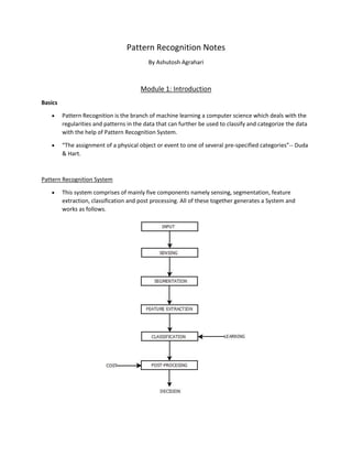
Pattern Recognition System
• This system comprises of mainly five components namely sensing, segmentation, feature
extraction, classification and post processing. All of these together generates a System and
works as follows.

2. Pattern Recognition System
1. Sensing and Data Acquisition: It includes, various properties that describes the object, such as its
entities and attributes which are captured using sensing device.
2. Segmentation: Data objects are segmented into smaller segments in this step.
3. Feature Extraction: In this step, certain features of data objects such as weight, colors,
dimension etc. are extracted.
4. Classification: Based on the extracted features, data objects are classified.
5. Post Processing & Decision: Certain refinements and adjustments are done as per the changes in
features of the data objects which are in the process of recognition. Thus, decision making can
be done once, post processing is completed.
Need : Pattern Recognition System
• Pattern Recognition System is responsible for generating patterns and similarities among given
problem/data space, that can further be used to generate solutions to complex problems
effectively and efficiently.
• Certain problems that can be solved by humans, can also be made to be solved by machine by
using this process.
Applications Of Pattern Recognition
1. Character Recognition.
2. Weather Prediction.
3. Sonar Detection.
4. Image Processing.
5. Medical Diagnosis.
6. Speech Recognition.
7. Information Management Systems.
Learning and Adaptation
• Learning and Adaptation can be collectively called as machine learning which can be defined as
the branch of computer science which enables computer systems to learn and respond to
queries on the basis of experience and knowledge rather than from predefined programs. Also,
it can be classified into supervised, unsupervised and reinforcement learning.
• Learning is a process in which the acquisition of knowledge or skills through study, experience,
or being taught.

3. • Adaptation refers to the act or process of adapting and adjustment to environmental conditions.
1. Learning and Adaptation : Supervised Learning
• When learning of a function can be done from its inputs and outputs, it is called as supervised
learning.
• One of the example of supervised learning is “Classification”.
• It classifies the data on the basis of training set available and uses that data for classifying new
data.
• The class labels on the training data is known in advance which further helps in data
classification.
Issues : Supervised Learning
• Data Cleaning: In data cleaning, noise and missing values are handled.
• Feature Selection: Abundant an irrelevant attributes are removed while feature selection is
done.
• Data Transformation: Data normalization and data generalization is included in data
transformation.
Classification Methods
• Decision Trees.
• Bayesian Classification.
• Rule Based Classification.
• Classification by back propagation.

4. • Associative Classification.
2. Learning and Adaptation : Unsupervised Learning
• When learning can be used to draw inference from some data set containing input data, it is
called as unsupervised learning.
• It clusters the data on the basis of similarities according to the characteristics found in the data
and grouping similar objects into clusters.
• The class labels on the training data is not known in advance i.e. no predefined class.
• The problem of unsupervised learning involves learning patterns from the inputs when specific
output values are supplied.
• Clustering is an example of unsupervised learning which can further be used on the basis of
different methods as per requirements.
Clustering Methods
• Hierarchical.
• Partitioning.
• Density Based.
• Grid Based.
• Model Based.
3. Learning and Adaptation : Reinforcement Learning
• Reinforcement in general is, the action or process of establishing a pattern of behavior.
• Hence, Reinforcement learning is the ability of software agents to learn and get reinforced by
acting in environment i.e. learning from rewards.
• In reinforcement learning, the software agents acts upon the environment and gets rewarded
for its action after evaluation but is not told, of which action was correct and helped it to
achieve the goal.
• For Example : Game Playing, Statistics.
Applications : Reinforcement Learning
• Manufacturing.
• Financial Sector.

5. • Delivery Management.
• Inventory Management.
• Robotics.
Pattern Recognition Approaches
• There are two fundamental pattern recognition approaches for implementation of pattern
recognition system. These are:
o Statistical Pattern Recognition Approaches.
o Structural Pattern Recognition Approaches.
Statistical Patter Recognition Approach
• Statistical Pattern Recognition Approach is in which results can be drawn out from established
concepts in statistical decision theory in order to discriminate among data based upon
quantitative features of the data from different groups. For example: Mean, Standard Deviation.
• The comparison of quantitative features is done among multiple groups.
• The various statistical approaches used are:
Statistical Pattern Recognition Approaches
1. Bayesian Decision Theory
• Bayesian decision theory is a statistical model which is based upon the mathematical foundation
for decision making.

6. • It involves probabilistic approach to generate decisions in order to minimize the complexity and
risk while making the decisions.
• In Bayesian decision theory, it is assumed that all the respective probabilities are known because
the decision problem can be viewed in terms of probabilities.
• It can be said that, Bayesian decision theory is dependent upon the Baye’s rule and
posterior probability needs to be calculated in order to make decisions with the knowledge of
prior probability. It can be calculated as :
Bayesian decision theory
• The difference is, Bayesian decision theory is the generalized form and can be used by replacing
the scalar ‘‘x’’ with the feature vector “X”.

7. Feature Vector : Bayesian Decision Theory
2. Normal Density
• Normal density curve is a bell shaped curve which is the most commonly used probability
density function.
Normal Density Curve : Pattern Recognition Approaches
• Since it is based upon the central limit theorem, normal density concept is able to handle larger
number of cases.

8. • The Central Limit Theorem States that - “A given sufficiently large sample size from a population
with a finite level of variance, the mean of all samples from the same population will be equal to
mean of population”.
• The normal density function can be given by:
Formula: Normal Density Function
3. Discriminant Function
• Pattern Classifiers can be represented with the help of discriminant functions.
• Discriminant Functions are used to check, which continuous variable discriminates between two
or more naturally occurring groups.
Structural Pattern Recognition Approach
• A Structural Approach is in which results can be drawn out from established concepts in
structural decision theory in order to check interrelations and interconnections between objects
inside single data sample.
• Sub-Patterns and relations are the structural features while applying an structural approach.
• For example : Graphs.

9. Chi-Squared Test
• Whenever, it is required to determine the correlation between two categorical variable,
statistical method i.e. Chi-Square test is used.
• The condition for this is, both the categorical variable must be fetched from same data sample
population and one should be able to categorize them on the basis of their properties in
either Yes/No, True/False etc.
• One of the simplest example is, we can correlate the gender of a person with the type of sport
they play on the basis of observation on a data set of sport playing pattern.
• Chi square test can be evaluated on the basis of below mentioned formula.

11. • For example:

12. Module 2: Statistical Pattern Recognition
Bayesian Decision Theory
Refer Bayesian Decision Theory.pdf
Classifiers
In a typical pattern recognition application, the raw data is processed and converted into a form that is
amenable for a machine to use. Pattern recognition involves classification and cluster of patterns.
In classification, an appropriate class label is assigned to a pattern based on an abstraction that is
generated using a set of training patterns or domain knowledge. Classification is used in supervised
learning.
Example: Naïve Bayes Classifier, KNN, SVM, Decision Trees, Random Forests, Logistic Regression
Discriminant Functions and Normal Density
Refer Discriminant Functions For The Normal(Gaussian) Density.pdf

13. Module 3: Parameter Estimation
• In order to estimate the parameters randomly from a given sample distribution data, the
technique of parameter estimation is used.
• To achieve this, a number a estimation techniques are available and listed below.
Parameter Estimation Techniques
• To implement the estimation process, certain techniques are available including Dimension
Reduction, Gaussian Mixture Model etc.
1. Maximum likelihood Estimation
• Estimation model consists of a number of parameters. So, in order to calculate or estimate the
parameters of the model, the concept of Maximum Likelihood is used.
• Whenever the probability density functions of a sample is unknown, they can be calculated by
taking the parameters inside sample as quantities having unknown but fixed values.
• In simple words, consider we want to calculate the height of a number of boys in a school. But, it
will be a time consuming process to measure the height of all the boys. So, the unknown mean
and unknown variance of the heights being distributed normally, by maximum likelihood
estimation we can calculate the mean and variance by only measuring the height of a small
group of boys from the total sample.
2. Bayesian Parameters Estimation
• “Parameters” in Bayesian Parameters Estimation are the random variable which comprises of
known Priori Distribution.

14. • The major objective of Bayesian Parameters Estimation is to evaluate how varying parameter
affect density estimation.
• The aim is to estimate the posterior density P(Θ/x).
• The above expression generates the final density P(x/X) by integrating the parameters.
Bayesian Parameter Estimation
3. Expectation Maximization(EM)
• Expectation maximization the process that is used for clustering the data sample.
• EM for a given data, has the ability to predict feature values for each class on the basis of
classification of examples by learning the theory that specifies it.
• It works on the concept of, starting with the random theory and randomly classified data along
with the execution of below mentioned steps.
o Step-1(“E”) : In this step, Classification of current data using the theory that is currently
being used is done.
o Step-2(“M”) : In this step, With the help of current classification of data, theory for that
is generated.
Thus EM means, Expected classification for each sample is generated used step-1 and theory is
generated using step-2.
Dimension Reduction
• Dimension reduction is a strategy with the help of which, data from high dimensional space can
be converted to low dimensional space. This can be achieved using any one of the two
dimension reduction techniques :
o Linear Discriminant Analysis(LDA)
o Principal Component Analysis(PCA)
1. Linear Discriminant Analysis(LDA)

15. • Linear discriminant analysis i.e. LDA is one of the dimension reduction techniques which is
capable of discriminatory information of the class.
• The major advantage of using LDA strategy is, it tries to obtain directions along with classes
which are best separated.
• Scatter within class and Scatter between classes, both are considered when LDA is used.
• Minimizing the variance within each class and maximizing the distance between the means are
the main focus of LDA.
Algorithm for LDA
• Let the number of classes be “c” and ui be the mean vector of class i, where i=1,2,3,.. .
• Let Ni be the number of samples within class i, where i=1,2,3…C.
Total number of samples, N=∑ Ni.
• Number of samples within Class Scatter Matrix.
• Number of samples between Class Scatter Matrix.

16. Advantages Of : Linear Discriminant Analysis
• Suitable for larger data set.
• Calculations of scatter matrix in LDA is much easy as compared to co-variance matrix.
Disadvantages : Linear Discriminant Analysis
• More redundancy in data.
• Memory requirement is high.
• More Noisy.
Applications : Linear Discriminant Analysis
• Face Recognition.
• Earth Sciences.
• Speech Classification.
2. Principal Component Analysis(PCA)
• Principal Component Analysis i.e. PCA is the other dimension reduction techniques which is
capable of reducing the dimensionality of a given data set along with ability to retain maximum
possible variation in the original data set.

17. • PCA standouts with the advantage of mapping data from high dimensional space to low
dimensional space.
• Another advantage of PCA is, it is able to locate most accurate data representation in
low dimensional space.
• In PCA, Maximum variance is the direction in which data is projected.
Algorithm For PCA
• Let d1,d2, d3,…,dd be the whole data set consisting of d-dimensions.
• Calculate the mean vector of these d-dimensions.
• Calculate the covariance matrix of data set.
• Calculate Eigen values(λ1,λ2,λ3,…,λd) and their corresponding Eigen vectors (e1, e2, e3,….ed).
• Now, Sort the Eigen vectors in descending order and then choose “p” Eigen vectors having
largest values in order to generate a matrix “A” with dimensions p*d.
i.e. A = d * p.
• Using the matrix “A” (i.e. A = d * p) in order to transform samples into new subspace with the
help of:
y = AT
* x
Where, AT
Transpose matrix of “A”
Advantages : Principal Component Analysis
• Less redundancy in data.
• Lesser noise reduction.
• Efficient for smaller
Disadvantages : Principal Component Analysis
• Calculation of exact co-variance matrix is very difficult.
• Not suitable for larger data sets.
Applications : Principal Component Analysis
• Nano-materials.
• Neuroscience.
• Biological Systems.

18. Hidden Markov Models (HMM)
• Markov model is an un-precised model that is used in the systems that does not have any fixed
patterns of occurrence i.e. randomly changing systems.
• Markov model is based upon the fact of having a random probability distribution or pattern that
may be analysed statistically but cannot be predicted precisely.
• In Markov model, it is assumed that the future states only depends upon the current states and
not the previously occurred states.
• There are four common Markov-Models out of which the most commonly used is the
hidden Markov-Model.
Hidden Markov Model(HMM)
• Hidden Markov-Model is an temporal probabilistic model for which a single discontinuous
random variable determines all the states of the system.
• It means that, possible values of variable = Possible states in the system.
• For example: Sunlight can be the variable and sun can be the only possible state.
• The structure of Hidden Markov-Model is restricted to the fact that basic algorithms can be
implemented using matrix representations.
Concept : Hidden Markov Model
• In Hidden Markov-Model, every individual states has limited number of transitions and
emissions.
• Probability is assigned for each transition between states.

19. • Hence, the past states are totally independent of future states.
• The fact that HMM is called hidden because of its ability of being a memory less process i.e. its
future and past states are not dependent on each other.
• Since, Hidden Markov-Model is rich in mathematical structure it can be implemented for
practical applications.
• This can be achieved on two algorithms called as:
1. Forward Algorithm.
2. Backward Algorithm.
Applications : Hidden Markov Model
• Speech Recognition.
• Gesture Recognition.
• Language Recognition.
• Motion Sensing and Analysis.
• Protein Folding.
Gaussian Mixture Models (GMM)
Gaussian mixture models are a probabilistic model for representing normally
distributed subpopulations within an overall population. Mixture models in general don't require
knowing which subpopulation a data point belongs to, allowing the model to learn the subpopulations
automatically. Since subpopulation assignment is not known, this constitutes a form of unsupervised
learning.
For example, in modeling human height data, height is typically modeled as a normal distribution for
each gender with a mean of approximately 5'10" for males and 5'5" for females. Given only the height
data and not the gender assignments for each data point, the distribution of all heights would follow the
sum of two scaled (different variance) and shifted (different mean) normal distributions. A model
making this assumption is an example of a Gaussian mixture model (GMM), though in general a GMM
may have more than two components. Estimating the parameters of the individual normal distribution
components is a canonical problem in modeling data with GMMs.

20. GMMs have been used for feature extraction from speech data, and have also been used extensively in
object tracking of multiple objects, where the number of mixture components and their means predict
object locations at each frame in a video sequence.
Learnt using EM algorithm.
EM for Gaussian Mixture Models
Expectation maximization for mixture models consists of two steps.
The first step, known as the expectation step or E step, consists of calculating the expectation of the
component assignments Ck for each data point xi in Xxi∈X given the model parameters ϕk, μk, and σk.
The second step is known as the maximization step or M step, which consists of maximizing the
expectations calculated in the E step with respect to the model parameters. This step consists of
updating the values ϕk, μk, and σk.
The entire iterative process repeats until the algorithm converges, giving a maximum likelihood
estimate. Intuitively, the algorithm works because knowing the component assignment C_kCk for each xi
makes solving for ϕk, μk, and σk easy, while knowing ϕk, μk, and σk makes inferring p(Ck|xi) easy. The
expectation step corresponds to the latter case while the maximization step corresponds to the former.
Thus, by alternating between which values are assumed fixed, or known, maximum likelihood estimates
of the non-fixed values can be calculated in an efficient manner.

21. Module 4: Non Parametric Techniques
• Density Estimation is a Non-Parameter Estimation technique which is used to determine the
probability density function for a randomly chosen variable among a data set.
• The idea of calculating unknown probability density function can be done by:
where,
“x” Denotes sample data i.e. x1, x2, x3,..,xn on region R.
P(X) denotes the estimated density and
P denotes the average estimated density .
• In order to calculate probability density estimation on sample data “x”, it can be achieved by:
• Histogram is one of the simplest way used for density estimation.
• Other approaches used for non-parametric estimation of density are:
o Parzen Windows.
o K-nearest Neighbor.
Parzen Windows

22. • Parzen windows is considered to be a classification technique used for non-parameter
estimation technique.
• Generalized version of k-nearest neighbour classification technique can be called as Parzen
windows.
• Parzen Windows algorithm is based upon the concept of support vector machines and is
considered to be extremely simple to implement.
• Parzen Windows works on the basis of considering all sample points of given sample data based
on scheme of voting and assigning weights w.r.t the kernel function. It does not consider
the neighbors and labelled weights.
• Also, it does not requires any training data as it can affect the speed of operation.
• Parzen windows decision function can be represented by:
where, P(X) is the Gaussian function which is also known as Parzen probability density estimation in 2-D.
K-Nearest Neighbor
• K-Nearest Neighbor is another method of non-parameter estimation of classification other than
Parzen Windows.
• K-Nearest Neighbor( also known as k-NN) is one of the best supervised statistical learning
technique/algorithm for performing non-parametric classification.

23. • In K-Nearest Neighbor algorithm, class of an object is determined on the basis of class of
its neighbor.
How It Works?
• Consider a training sample of Squares and circles and circles. Now we need to classify the “Star”
Shape on the basis of its neighbors i.e. Squares and Circles.
• Let xi be the training sample and “k” be the distance from the position of “Star” shape.
Disadvantages : Using K-NN
• Expensive.
• High Space Complexity.
• High Time Complexity.
• Data Storage Required.
• High-Dimensionality of Data.

24. Fuzzy Classification
A classifier is an algorithm that assigns a class label to an object, based on the object description. It is also
said that the classifier predicts the class label. The object description comes in the form of a vector
containing values of the features (attributes) deemed to be relevant for the classification task. Typically,
the classifier learns to predict class labels using a training algorithm and a training data set. When a
training data set is not available, a classifier can be designed from prior knowledge and expertise. Once
trained, the classifier is ready for operation on unseen objects.
Any classifier that uses fuzzy sets or fuzzy logic in the course of its training or operation is known as fuzzy
classifier.
For example, a person who is dying of thirst in the desert is given two bottles of fluid. One bottle’s label
says that it has a 0.9 membership in the class of fluids known as non-poisonous drinking water. The other
bottle’s label states that it has a 90% probability of being pure drinking water and a 10% probability of
being poison. Which bottle would you choose?
In the example, the "probability bottle" contains poison. This is quite plausible since there was a 1 in 10
chance of it being poisonous. The "fuzzy bottle" contains swamp water. This also makes sense since
swamp water would have a 0.9 membership in the class of non-poisonous fluids. The point is that
probability involves crisp set theory and does not allow for an element to be a partial member in a class.
Probability is an indicator of the frequency or likelihood that an element is in a class. Fuzzy set theory
deals with the similarity of an element to a class.

25. Module 5: Unsupervised Learning and Clustering
K-Means Clustering
• K-Means clustering is known to be one of the simplest unsupervised learning algorithms that is
capable of solving well known clustering problems.
• K-Means clustering algorithm can be executed in order to solve a problem using four simple
steps:
o Make the partition of objects into K non empty steps i.e. K=1,2,3,.. .
o Consider arbitrary seed points from sample data.
o Calculate mean distance of sample data from seed points in order to generate clusters.
o Repeat the above steps until values of two clusters becomes same. Below is an solved
example.

26. Criterion Function : Clustering
• To measure the quality of clustering ability of any partitioned data set, criterion function is used.
• Consider a set , B = { x1,x2,x3…xn} containing “n” samples, that is partitioned exactly into “t”
disjoint subsets i.e. B1, B2,…..,Bt.
• The main highlight of these subsets is, every individual subset represents a cluster.
• Sample inside the cluster will be similar to each other and dissimilar to samples in other clusters.
• To make this possible, criterion functions are used according the occurred situations.
Criterion Function For Clustering
1. Internal Criterion Function
• This class of clustering is an intra-cluster view.
• Internal criterion function optimizes a function and measures the quality of clustering ability
various clusters which are different from each other.
2. External Criterion Function
• This class of clustering criterion is an inter-class view.
• External Criterion Function optimizes a function and measures the quality of clustering ability of
various clusters which are different from each other.
3. Hybrid Criterion Function
• This function is used as it has the ability to simultaneously optimize multiple individual Criterion
Functions unlike as Internal Criterion Function and External Criterion Function.

27. Iterative Square error clustering methods
The most commonly used clustering strategy is based on the square-root error criterion.
Objective: To obtain a partition which, for a fixed number of clusters, minimizes the square-error where
square-error is the sum of the Euclidean distances between each pattern and its cluster center.
Algorithm
1. Select an initial partition with k clusters. Repeat steps 2 through 5 until the cluster membership
stabilizes.
2. Generate a new partition by assigning each pattern to its closest cluster center.
3. Compute new cluster centers as the centroids of the clusters.
4. Repeat steps 2 and 3 until an optimum value of the criterion is found.
5. Adjust the number of clusters by merging and splitting existing clusters or by removing small or
outlier clusters.
The algorithm converges when the criterion function cannot be improved.
Initial partition
• Select k seed points at random or by taking the centroid as the first seed point and the rest at a
certain miminimum distance from this seed point.
• Cluster the remaining points to the closest seed point.
Updating a partition
K-means:
• In each pass(cycle) make an assignment of all patterns to the closest cluster center.
• Recompute the cluster center after every new assignment is made.
Adjusting the number of clusters
• Clustering algorithms can create new clusters or merge existing ones if certain conditions
specified by the user are met.
• Split a cluster if it has too many patterns and an unusually large variance along the feature with
large spread.
• Merge if they are sufficiently close.

28. • Remove outliers from future consideration. (outliers are pattern/patterns that is sufficiently far
removed from the rest of the data and hence suspected as a mistake in data entry.)
Performance of square-error clustering methods
• Seeks compact hyper-ellipsoidal clusters and this can produce misleading results when the data
do not occur in compact, hyper-ellipsoidal boundaries.
• Exhibit inadequacies when the Euclidean measure is used to measure distance but the features
are not on comparable scales.
Agglomerative Hierarchical Clustering
Agglomerative clustering is a strategy of hierarchical clustering. Hierarchical clustering (also known as
Connectivity based clustering) is a method of cluster analysis which seeks to build a hierarchy of clusters.
Hierarchical clustering, is based on the core idea of objects being more related to nearby objects than to
objects farther away. As such, these algorithms connect 'objects' to form clusters based on their
distance. A cluster can be described largely by the maximum distance needed to connect parts of the
cluster. At different distances, different clusters will form, which can be represented using a
dendrogram, which explains where the common name 'hierarchical clustering' comes from: these
algorithms do not provide a single partitioning of the data set, but instead provide an extensive
hierarchy of clusters that merge with each other at certain distances. In a dendrogram, the y-axis marks
the distance at which the clusters merge, while the objects are placed along the x-axis so the clusters
don't mix.
Strategies for hierarchical clustering generally fall into two types:
• Agglomerative: This is a bottom-up approach: each observation starts in its own cluster, and
pairs of clusters are merged as one moves up the hierarchy.
• Divisive: This is a top-down approach: all observations start in one cluster, and splits are
performed recursively as one moves down the hierarchy.
Hierarchical clustering is a whole family of methods that differ by the way distances are computed.
Apart from the usual choice of distance functions, the user also needs to decide on the linkage criterion
to use, since a cluster consists of multiple objects, there are multiple candidates to compute the
distance to. Popular choices are known as single-linkage clustering (the minimum of object distances),
complete-linkage clustering (the maximum of object distances) or average-linkage clustering (also
known as UPGMA, 'Unweighted Pair Group Method with Arithmetic Mean').
The algorithm forms clusters in a bottom-up manner, as follows: Initially, put each example in its own
cluster. Among all current clusters, pick the two clusters with the smallest distance. Replace these two
clusters with a new cluster, formed by merging the two original ones. Repeat the above two steps until
there is only one remaining cluster in the pool.

29. Clustering is concerned with grouping together objects that are similar to each other and dissimilar to
the objects belonging to other clusters. It is a technique for extracting information from unlabeled data
and can be very useful in many different scenarios e.g. in a marketing application we may be interested
in finding clusters of customers with similar buying behavior.
Cluster Validation
The term cluster validation is used to design the procedure of evaluating the goodness of clustering
algorithm results. This is important to avoid finding patterns in a random data, as well as, in the situation
where you want to compare two clustering algorithms.
Generally, clustering validation statistics can be categorized into 3 classes (Charrad et al. 2014,Brock et
al. (2008), Theodoridis and Koutroumbas (2008)):
1. Internal cluster validation, which uses the internal information of the clustering process to
evaluate the goodness of a clustering structure without reference to external information. It can
be also used for estimating the number of clusters and the appropriate clustering algorithm
without any external data.
2. External cluster validation, which consists in comparing the results of a cluster analysis to an
externally known result, such as externally provided class labels. It measures the extent to which
cluster labels match externally supplied class labels. Since we know the “true” cluster number in
advance, this approach is mainly used for selecting the right clustering algorithm for a specific
data set.

30. 3. Relative cluster validation, which evaluates the clustering structure by varying different
parameter values for the same algorithm (e.g.,: varying the number of clusters k). It’s generally
used for determining the optimal number of clusters.