Physics_150612_01

© Art Traynor 2011
Physics
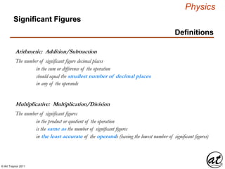
Significant Figures
Definitions
Arithmetic: Addition/Subtraction
The number of significant figure decimal places
in the sum or difference of the operation
Multiplicative: Multiplication/Division
The number of significant figures
in the product or quotient of the operation
should equal the smallest number of decimal places
in any of the operands
is the same as the number of significant figures
in the least accurate of the operands (having the lowest number of significant figures)

© Art Traynor 2011
Physics
Significant Figures
Definitions
Arithmetic: Addition/Subtraction
The number of significant figure decimal places
in the sum or difference of the operation
should equal the smallest number of decimal places
in any of the operands
Example:
123
+ 5.35
≠ 128.35
= 128
3 Sig Figs, 0 Decimal Places
3 Sig Figs, 2 Decimal Places
5 Sig Figs > 3 Sig Figs (2 Decimals)
3 Sig Figs, 0 Decimals

© Art Traynor 2011
Physics
Significant Figures
Definitions
L
W
Example:
L : 16.3cm ± 0.1cm { 16.2cm – 16.4cm }
W : 4.5cm ± 0.1cm { 4.4cm – 4.6cm }
A = l x w
A : 16.3cm
x 4.5cm
≠ 73.35cm 2 { 71cm – 75cm }
= 73cm 2
3 Sig Figs
2 Sig Figs
Multiplicative: Multiplication/Division
The number of significant figures
in the product or quotient of the operation
is the same as the number of significant figures
in the least accurate of the operands (having the lowest number of significant figures)
4 Sig Figs > 2 Sig Figs
2 Sig Figs
Serway, pg 15

© Art Traynor 2011
Physics
Significant Figures
Rules
Computational Rules
for Determining/Identifying Significant Figures
 All non-zero digits are considered significant
 Zeros bounded by non-zeros are significant
 Leading zeros are not significant
 Trailing zeros following a decimal point are significant
 Trailing zeros not accompanied by a decimal point are ambiguous
 A decimal point may be placed after the number
to ratify the significance of the trailing zeros
Wikipedia
 The least digit of a measurement is considered to be uncertain
Measurement Rules
for Determining/Identifying Significant Figures
Sect 1.5, pg 8
n = number of sig fig, n – 1 = figures of certainty
 Integers or Fractions are considered to be significant Sect 1.5, pg 9

© Art Traynor 2011
Physics
Significant Figures
Rounding
 Substituting a fractional decimal number by one with fewer digits
There are at least six (6) canonical forms to which the principles of Rounding apply.
Rounding
 Round to Specified Increment
There are at least two (2) rounding methodologies
 Round to Integer
There are at least four (4) functions which produce round-to-integer results
 Round Up – apply the ceiling function, or round towards +∞
Ceiling Function
Assigns to the real number x
the smallest integer that is greater than or equal to x
Examples: ⌈3.1⌉ = 4 ; ⌊ – 0.5⌋ = 0 ; ⌈7⌉ = 7
⌈x⌉ = ℤ ≥ x
Rosen, pg 149

© Art Traynor 2011
Physics
Significant Figures
Rounding
Rounding
 Round to Integer
There is at least one (1) non-direct method to produce round-to-integer results
 Round To Nearest – “ q” is the integer that is closest to “ y”
“ y” is the number to be rounded ( y ℝ )
“ q” is the integer result ( q ℤ ) of the rounding operation
Some “ tie-breaking” rule is required
for when “ y” is half-way between two integers, i.e. y = 0.5
n Round Half-Up or round half towards +∞
q = : ⌊ y + 0.5⌋ = – ⌈ – y – 0.5⌉
Examples: ⌊ 23.5 + 0.5⌋ = 24 ;
– ⌈ – ( – 23.5 ) – 0.5⌉ = – 23
Rosen, pg 149


© Art Traynor 2011
Physics
Measurement
SI Units
10 – 24
10 – 21
10 – 18
10 – 15
10 – 12
10 – 9
10 – 6
10 – 3
10 – 2
10 – 1
Yocto y 10 24YottoY
Zepto z 10 21ZettaZ
Atto a 10 18ExaE
Fempto f 10 15PetaP
Pico P 10 12TeraT
Nano n 10 9GigaG
Micro μ 10 6MegaM
Milli m 10 3Kilok
Centi c 10 2
Deci d 10 1Dekada
Hectoh
Systèm Internationale ( SI )
Unit Prefixes

© Art Traynor 2011
Physics
Uncertainty
Precision & Accuracy
Accuracy
The degree of closeness to which a quantitative measurement
approximates the true value of the quantity measured
Precision
The degree to which repeated measurements (under unchanged conditions)
yield the same results
Significant Figure Representation
Margin of error is presumed to constitute
one-half the value of the last significant place
Examples: 843.6m or 843.0m or 800.0m
implies a margin of error of 0.05m or ± 0.05m
843.55m ≤ x ≤ 843.65m (nominal 843.6m)
842.95m ≤ x ≤ 843.05m (nominal 843.0m)
800.95m ≤ x ≤ 800.05m (nominal 840.0m)

© Art Traynor 2011
Physics
Uncertainty
Approximation Error
Approximation Error
The discrepancy between an exact value
and some approximation ( measurement ) of it
Absolute Error ( Tolerance )
The magnitude of the difference
between the exact value
and the approximation ( e.g. ± 0.05m )
Magnitudes are always expressed
as absolute values and are thus
always positive numbers
Relative/Fractional/Percentage Error
The absolute error expressed
as a ratio of the exact value ( e.g. 56.47 ± 0.02mm )
0.02mm
56.47mm
=
Absolute Error
Exact Value
= 0.0004 → ( 0.0.0.04 ) ( 100% ) = 0.04%
Relative Error ➀ ➁ Percentage Error

© Art Traynor 2011
Physics
Scientific Notation
Exponentiation
Scientific Notation (Generally)
whereby a number with a surfeit of zeros (either large or small in relative magnitude)
or otherwise populated by digits beyond those necessary for the desired precision (significant figures)
A species of mathematic operation (exponentiation)
is alternatively expressed as the product of a coefficient (reduced to only its significant figures)
and a multiplier-constant (ten) indexed by an integer.
a x 10b
Normalized Scientific Notation
one and ten, 1 ≤ |a | < 10 , which allows for easy comparison of two numbers so expressed
as the exponent b in this form represents the product’s order of magnitude
In NSN the exponent b is chosen so that the absolute value of the coefficient a is bounded between
 For numbers with absolute value between zero and one, 0 < |a | < 1
the exponent b, is expressed as a negative index (e.g. – 5 x 10-1 )
Examples: – 0.5 = – 0.5.0 = – 5.0 x 10-1
➀
Moving 1 position
in the “–” direction
Wikipedia
Representing a decimal by
scientific notation (resultant)
entails movement of the
decimal in the “ – “ direction

© Art Traynor 2011
Physics
Scientific Notation
Exponentiation
a x 10b
Engineering Scientific Notation
a lies between one and one-thousand, 1 ≤ |a | < 1000 , which allows for easy comparison of
two numbers so expressed as the exponent b corresponds to specific SI prefixes
In ESN the exponent b is restricted to multiples of three so that the absolute value of the coefficient
Example: “ 0.0000000125m ” →
 12.5 x 10-9m “ twelve-point-five nanometers ”
 1.25 x 10-8m “ one-point-two-five times ten-to-the-negative-eight meters ”
⑨
( 0.0.0.0.0.0.0.0.1.25 ) = 1.25 x 10-8 m
⑧① ②③ ④ ⑤⑥ ⑦
Moving 8 positions
( 0.0.0.0.0.0.0.0.1.2.5 ) = 12.5 x 10-9 m
⑧① ②③ ④ ⑤⑥ ⑦
Moving 9 positions
Wikipedia
Representing a decimal by
decimal in the “ – “ direction

© Art Traynor 2011
Physics
Scientific Notation
Exponentiation
a x 10b
Example: “ 350 ”
 350 = 3.5.0.0 = 3.5 x 102


Representing integers by
decimal in the “ + “ direction
①②
Moving 2 positions
in the “+” direction
350 = 35.0.0 = 35.0 x 101
①
Moving 1 position
350 = 350.0 = 350.0 x 100
i
Moving 0 positions

© Art Traynor 2011
Physics
Properties of Substances
Density
Density : r (rho)
A fundamental property of any substances is its density.
Density is the mass per unit volume of any substance
r =
m
V
 Densities do not necessarily correlate to atomic masses
 Atomic spacings and crystalline structure affect elemental density
 Avagadro’s Number
 Specific Gravity

© Art Traynor 2011
Physics
Definition
Vectors
Vector (Euclidean)
A geometric object (directed line segment)
describing a physical quantity and characterized by
Direction: depending on the coordinate system used to describe it; and
Magnitude: a scalar quantity (i.e. the “length” of the vector)
Aka: Geometric or Spatial Vector
originating at an initial point [ an ordered pair : ( 0, 0 ) ]
and concluding at a terminal point [ an ordered pair : ( ax , ay ) ]
Other mathematical objects
describing physical quantities and
coordinate system transforms
include: Pseudovectors and
Tensors
 Not to be confused with elements of Vector Space (as in Linear Algebra)
 Fixed-size, ordered collections
 Aka: Inner Product Space
 Also distinguished from statistical concept of a Random Vector
From the Latin Vehere (to carry)
constituting the components of the vector 〈 ax , ay 〉

© Art Traynor 2011
Physics
Vectors
Vector (Euclidean) Aka: Geometric or Spatial Vector
 Free Vector
a vector without a fixed origin defined by some coordinate system
which can be adequately described by Direction & Magnitude alone
 Bound (Position) Vector
a vector whose origin is fixed and located by some coordinate system
Coordinate systems (other than
Cartesian) include: Cylindrical,
and Spherical
 Determinant Form
a representation of a vector in Rn space by a 1 x n column matrix the
entries of which are the coefficients of the unit vectors ( )
from which vector components can be derived
k^j^i^
Representation

© Art Traynor 2011
Physics
Vectors
initial point
terminal point
x
y
║a ║
Free Vector Bound Vector
initial point
terminal point
║a ║
 Free Vector
a vector without a fixed origin defined by some coordinate system
which can be adequately described by Direction & Magnitude alone
 Bound Vector
a vector whose origin is fixed and located by some coordinate system
Coordinate systems (other than
Cartesian) include: Cylindrical,
and Spherical
Representation

© Art Traynor 2011
Physics
Representation
Vectors
Vector (Euclidean)
 Determinant Form
Col. 1
a1
a =
a2
a3
an
.
.
.
A vector a = 〈 a1 , a2 , a3 … an 〉 , in Rn space can be represented
by an 1 x n column matrix

© Art Traynor 2011
Physics
Definition
Vectors
Vector (Euclidean)
A geometric object (directed line segment)
describing a physical quantity and characterized by
Direction: depending on the coordinate system used to describe it; and
Magnitude: a scalar quantity
originating at initial point and concluding at a terminal point
initial point
terminal point
x
y
║a ║
Free Vector Bound Vector
initial point
terminal point
║a ║
( 0, 0 )
( ax , ay )
( 0, 0 )
( ax , ay )

© Art Traynor 2011
Physics
Vectors
PQ
x
y Position Vector
initial point
terminal point
║a ║
O
θ
A ( ax , ay )
initial point
terminal point
║a ║
Free Vector
Q
P
 Position Vector Form (PVF)
For any vector possessing Direction & Magnitude
there is precisely one equivalent Position Vector a = OA
a
with an initial point situated at the coordinate system origin
and extending to terminal point ( ax , ay )
PVF: Position Vector Form
Position Vector

© Art Traynor 2011
Physics
Vectors
PQ
x
y Position Vector
║a ║
O
θ
A ( ax, ay )
initial point
terminal point
║a ║
Free Vector
Q
P
 Position Vector - Properties
The property of vector Direction further implies the property of Angularity
between vectors or coordinate system axes
a
Each (position) vector determines a unique Ordered Pair ( ax , ay )
The coordinates a1 and a2 form the Components of vector 〈 ax , ay 〉
ax
ay



Position Vector
opp
adj( )θ = tan-1
ay
ax
( )= tan-1
If we know ay and ax we can always
find the angle in between ( the
orientation of the position vector )
by computing an arctangent of the
two component vectors
Eq. 1.8 ( Pg. 16 )

© Art Traynor 2011
Physics
Magnitude
Vectors
x
y
O
θ
A ( ax , ay )
 Magnitude
a
Position Vector
xO
θ
a (adj )
b (opp )
r = c (hyp )
M A (1, 0)
P ( cos θ, sin θ )
1
tan θ
cos θ
Q
sin θ
y
UCF: Unit Circle Form
ay
ax
Unit Circle - QI
In PVF the magnitude of a vector a = 〈 ax , ay 〉 is equivalent to the
hypotenuse ( c = ║a ║ ) of a right triangle whose adjacent side
( a ) is given by the coordinate a1 , and whose opposite side ( b )
is given by the coordinate a2 :
2 2
ax + ay║a ║ = ║ 〈 ax , ay 〉 ║ =
Pythagorean Theorem derived

© Art Traynor 2011
Physics
Vectors
x
y Position Vector
O
θ
A ( ax, ay )
 Vector – Components
In PVF a vector can be “resolved” or “decomposed” into its
constituent horizontal “ x ” and vertical “ y ” elements the
projection of which onto the coordinate axes form the horizontal
and vertical components of the vector.
ax
ay

A
Ay
Ax
xO
θ
a (adj )
b (opp )
r = c (hyp )
M A (1, 0)
1
tan θ
cos θ
Q
sin θ
y Unit Circle - QI
b
c
sin θ =
opp
hyp( )
a
c
cos θ =
adj
hyp( )
b
a
tan θ =
opp
adj( )
tan θ = sin θ
cos θ( )
Sine is Prime and that’s why it Rhymes*
“A” is ayyyydjacent…*
It’s obeeevious that “B” is opposite
*
Components
opp
adj( )θ = tan-1
ay
a1
( )= tan-1
Eq. 1.8 ( Pg. 16 )

© Art Traynor 2011
Physics
Vectors
Vector (Euclidean)
x
y Position Vector
O
θ
A ( ax , ay )

AAy
Ax
xO
θ
a (adj )
b (opp )
r = c (hyp )
M A (1, 0)
1
tan θ
cos θ
Q
sin θ
y Unit Circle - QI
b
c
sin θ =
opp
hyp( )
a
c
cos θ =
adj
hyp( )
Ay = y component of A = ║A ║ sinθ
Ax = x component of A = ║A ║ cosθ
║A ║ cos θ
║A║sinθ
Warning
Only applicable to
resolved/decomposed vector
Components
opp
adj( )θ = tan-1
ay
ax
( )= tan-1
*
Eq. 1.8 ( Pg. 16 )

© Art Traynor 2011
Physics
Vectors
Vector (Euclidean)
x
y Position Vector
O
θ

Components
Ay
Ax
xO
θ
a (adj )
b (opp )
r = c (hyp )
M A (1, 0)
1
tan θ
cos θ
Q
sin θ
y Unit Circle - QI
Ay = y component of A = ║A ║ sinθ
Ax = x component of A = ║A ║ cosθ
║A ║ cos θ
║A║sinθ
Vector resolution/decomposition
always presupposes a coordinate system
they are not vectors themselves,
Trigonometric functions (sin, cos, tan, etc.)
of the vector components therefore
relate only to the resolved/decomposed vector
and not to any angle or trigonometric function
of some other operand vector(s)
A ( ax , ay )
A
sin θ =
opp
hyp( )
cos θ =
adj
hyp( )
Warning
Only applicable to
resolved/decomposed vector
opp
adj( )θ = tan-1
ay
ax
( )= tan-1
*
Eq. 1.8 ( Pg. 16 )

© Art Traynor 2011
Physics
Vectors
Vector (Euclidean)
PQ
x
y Position Vector
O initial point
Free Vector
C
 Vector Scalar Multiple

Physical Quantities represented
by vectors include: Displacement,
Velocity, Acceleration, Momentum,
Gravity, etc.
O
C ( cax , cay )
A ( ax , ay )
c OA = OC
terminal point
Example: F = ma
Vector Scalar Multiple
Operands are oriented “ tip-to-tail ”
with the multiplicand ( vector to be
scaled ) “ scaled ” by the
multiplier-scalar.
The result constitutes a vector
addition of the product of the
scalar and the multiplicand
normalized unit vector (NUV) thus
preserving multiplicand orientation
in the result
c 〈 ax , ay 〉 = 〈 cax , cay 〉

© Art Traynor 2011
Physics
Vectors
Vector (Euclidean)
x
y Position Vector
O
θ
A ( ax , ay )
 Unit Vector (Components)
Any vector in PVF can be expressed as a scalar product of the vector
sum of its unit (multiplicative scalar identity) components
î = 〈 1, 0 〉 , ĵ = 〈 1, 0 〉
a
ĵ
î x
y Position Vector
O
θ
A ( ax , ay )
ay ĵ
ax î
a
a = ax î + ay ĵ
c ( î ) = 〈 c1, c0 〉 , c ( ĵ ) = 〈 c 0, c 1 〉
ax ( î ) = 〈 ax 1, ax 0 〉 , ay ( ĵ ) = 〈 ay 0, ay 1 〉
Unit Vector

© Art Traynor 2011
Physics
Vectors
Aka: Versor (Cartesian)
x
y Position Vector
O
θ
 Normalized Unit Vector
A normalized unit vector (NUV) is the vector of unitary magnitude
corresponding to the set of all vectors which share its direction
ĵ
î x
y Position Vector
O
θ
A ( ax, ay )
a2 ĵ
a1 î
A ( ax , ay )
û ( ax , ay )║a ║
1
║a ║
1

Any vector can be specified by the scalar product of its corresponding
normalized unit vector and its magnitude (identity)

a = ax î + ay ĵ
1
║a ║
a
║a ║
û = a =
The NUV of a vector is the scalar product of the reciprocal of its magnitude
ĵ
î
û
ûa
Normalized Unit Vector

© Art Traynor 2011
Physics
Vectors
PQ
x
y Bound Vector
initial point
terminal point
║a ║
O
θ
A ( ax , ay )
initial point
terminal point
║a ║
Free Vector
Q
P
 Equivalent Vector
 Any vector possessing the same Direction & Magnitude as another
 Irrespective of Location within a coordinate system
a
PQ = a
Equivalent Vector

© Art Traynor 2011
Physics
Equivalent Vector
Vectors
Vector (Euclidean)
x
y Position Vector
O initial point
terminal point
Free Vector
R
A
 Equivalent Vector
 The sum of a pair of two equivalent vectors form a parallelogram
B
Gravity, etc.
OA + OB = OR
O
r ( ax+ bx , ay + by )
a ( ax, ay )
b ( bx , by )
 Vector Sum
║a ║
║b ║
║a ║ + ║b ║ ≠ ║r ║
 The sum of two vectors is the sum of their components
 A sum of vectors is not equal to the sum of their magnitudes
Because of the angle between
them! Only when vectors are
parallel (share the same direction)
will their magnitude sum equal
their vector sum.
║r ║= ║〈( ax + bx ), ( ay + by ) 〉║
( ax + bx ) 2 + ( ay + by ) 2=
θ = tan -1
ax + bx
ay + by
( )“ Angle Between ”
Orientation of
Resultant Vector
resultant vector is oriented “ tip-to-
tip ”

© Art Traynor 2011
Physics
Vectors
x
y
Corresponding Vector
initial point
terminal point
║a ║
O
θ
A ( ax , ay )
 Vector Correspondence
 Any vector possessing the same Direction & Magnitude as another
 The vector a that corresponds to any points P1( x1 , y1 ) and
P2( x2 , y2 ) P1 P2 is a = 〈 x2 – x1 , y2 – y1 〉
a
║P1 P2 ║
P2 ( x2 , y2 )
P1 ( x1 , y1 )
Correspondence

© Art Traynor 2011
Physics
Addition
Vectors
Vector (Euclidean)
x
y
O initial point
terminal point
Free Vector
r
A
 Sum of Vectors – Vector Addition (Tail –to–Tip)
B
O
a ( ax , ay )
b ( bx , by )
║a ║
║b ║
 Any two (or more) vectors can be summed by positioning the operand
vector (or its corresponding-equivalent vector) tail at the tip of the
augend vector.
 The summation (resultant) vector is then extended from (tail) the
origin (tail) of the augend vector to the terminal point (tip) of the
operand vector (tip-to-tip/head-to-head).
ry
rx
r ( rx , ry )
θ
θ = tan-1( tan θ )
θ = tan-1 opp
adj( )
θ = tan-1
ry
rx
( )
“ Tail-to-Tip ”
“ Tip-to-Tip ”
Same procedure, sequence of
operations whether for vector
addition (summation) or vector
subtraction (difference)
Resultant is always tip-to-tip
θ = tan -1
ax + bx
ay + by
Orientation of
Resultant Vector
tip ”

© Art Traynor 2011
Physics
Subtraction
Vectors
Vector (Euclidean)
x
y
O
ry
rx
θ
initial
point
terminal point
Free Vector
r = a + bcorr
a
b
O
“ Tail-to-Tip ”
“ Tip-to-Tip ”
( Addition )
bcorr
– bcorr “ Tip-to-Tip ”
( Difference )
Position Vector
r = a – bcorr
Difference of Vectors – Vector Subtraction ( Tail –to–Tip )
 Any two (or more) vectors can be subtracted by positioning the tail of
a corresponding-equivalent subtrahend vector (initial point) at the
tip (terminal point) of the minuend vector.
 The difference (resultant) vector is then extended from the tail (initial
point ) of the minuend vector (tail-to-tail) to the terminal point
(tip) of the subtrahend vector (tip-to-tip).
minuend
subtrahend
Same procedure, sequence of
operations whether for vector
addition (summation) or vector
subtraction (difference)
r
r = a + bcorr
bcorr
– bcorr
a
b
θ = tan-1
ry
rx
( )
θ = tan -1
ax + bx
ay + by
Orientation of
Resultant Vector
tip ”

© Art Traynor 2011
Physics
Vector Properties
a + b = b + a Commutative
Vectors
( a + b ) + c = a + ( b + c ) Associative, Additive
( cd ) a = c ( da )
Associative, Multiplicative
( cd ) a = d ( ca )
c ( a + b ) = ca + cb
Distributive
( c + d )a = ca + da
a – b = a + ( – b ) Difference
Re-Orders Terms
Does Not Change
Order of Operations – PEM-DAS
Changes Order of Operations
as per “PEM-DAS”, Parentheses
are the principal or first operation
Parenthesis are the “first to fight”
Always entails parentheses
Vector Properties

© Art Traynor 2011
Physics
Vector Properties
Vector Properties
a + 0 = a Additive Identity
Vectors
1 ( a ) = a Multiplicative Identity
a + ( – a ) = 0 Additive Negation
0a = 0
Multiplicative Zero Element
c0 = 0
– 1 ( a ) = – a
Multiplicative Inverse
– c 〈 ax , ay 〉 = 〈 – cax , – cay 〉

© Art Traynor 2011
Physics
Vectors
x
y Position Vector
O initial point
terminal point
Free Vector
A
B
O
A ( ax , ay )
B ( bx , by )
║a ║
║b ║
Vector (Euclidean)
 Dot Product
The dot product of two vectors
is the scalar summation
of the product
UCF: Unit Circle Form
a · b = ax bx + ay by
of their components, a = 〈 ax , ay 〉 , b = 〈 bx , by 〉
Also referred to as the Scalar Product or Inner Product Pythagorean Theorem derived
Dot Product

© Art Traynor 2011
Physics
Vectors
Col. 1 Col. 2 Col. 3 . . . Col. n
a1 a2 a3 . . . ana · b = aTb =
Col. 1
b1
b2
b3
bm
.
.
.
Vector (Euclidean)
 Dot Product ( Determinant Form )
The dot product of two vectors, is the matrix product
of the 1 x n transpose of the multiplicand vector
and the m x 1 multiplier vector
Col. 1
b1
b =
b2
b3
bm
.
.
.
Col. 1
a1
a =
a2
a3
an
.
.
.
a · b = aTb = a1b1 + a2b2 + a3b3 …+ anbm
Dot Product

© Art Traynor 2011
Physics
Dot Product Properties
Vector Dot Product Properties
a · a = ║a ║
2
Vector Square Identity
Vectors
a · b = b · a Commutative
a ( b + c ) = a · b + a · c Distributive
( ca ) · b = c ( a · b )
( ca ) · b = a · ( cb )
Distributive
Multiplicative Zero Element0 · a = 0

© Art Traynor 2011
Physics
Vectors
x
y Position Vector
O initial point
terminal point
Free Vector
A
B
O
A ( ax , ay )
B ( bx , by )
║a ║
║b ║
Vector (Euclidean)
 Dot Product & Angle Between Vectors
For any two non-zero vectors sharing a common initial point
the dot product of the two vectors is equivalent to
the product of their magnitudes and the cosine of the angle between
Dot Product
θ θ
a · b = ║b ║║a ║ cosθ
cosθ =
║a ║║b ║
a · b
You will be asked to find the angle
between two vectors sharing a
common initial point (origin)…a lot
Clarify how the difference of the
tangents could be used to find
angle between??

© Art Traynor 2011
Physics
Vectors
x
y Position Vector
O
Free Vector
Gravity, etc.
O
A ( ax , ay )
B ( bx , by )
a
b
c
A
B
θ θ
║a ║ cos θ
Vector (Euclidean)
a · b = ║b ║║a ║ cosθ
= a · b
OB – OA = AB
Dot Product

© Art Traynor 2011
Physics
Vectors
x
y
Position Vector
O
Free Vector
Gravity, etc.
O
A ( a1, a2 )
B ( b1x , by )
a
b
c
A
B
θ θ
║a ║ cos θ
║b ║
Area = ║b ║║a ║ cosθ
= a · b
Vector (Euclidean)
OB – OA = AB
Dot Product

© Art Traynor 2011
Physics
Vectors
xO
Gravity, etc.
O
A ( ax , ay )
B ( b1, b2 )
a
b
c
A
Bθ θ
║a ║ cos θ
 Vector Component Along an Adjoining Vector
Vector (Euclidean)
y
Position Vector
The component of OA along OB
that has the same direction as OB
║b ║
1
compb a = a · b
x
y
Position Vector
║b ║
b
compb a = a ·
Compb a = a ·║b ║
b
is the dot product of OA with the unit vector 1
║u ║
u
║a ║
û = u =( (
Dot Product

© Art Traynor 2011
Physics
Vectors
a1
b1
a2
b2
a3
b3
ay
by
az
bz
= [ ( aybz ) – ( azby ) ] î …–
ay
by
az
bz
C2 C3C1 C2 C3
C1
–
ax
bx
az
bz
C1 C3
C2
ax
bx
ay
by
C1 C2
C3
= k^
a x b = ( aybz – azby )i – ( axbz – azbx )j + ( axby – aybx )k^ ^ ^
a
b
a
b
Cross Product
① ②
C1
C2 C3
① ② –i ,^ –
1. Cross Product components are
the difference of the product of
the matrix diagonals
① ② +j ,^ ① ②
Vector Components1 Vector Magnitude
[( aybz – azby )]2
+ [ – ( axbz – azbx )]2
…
–
 Vector or Cross Product ( Determinant Form )
For any two non-zero vectors sharing a common initial point and angle between,
the vector or cross product yields a unique component set
describing a vector orthogonal to the operand vectors

© Art Traynor 2011
Physics
Vectors
 Vector or Cross Product ( Determinant Form )
For any two non-zero vectors sharing a common initial point and angle between,
the vector or cross product yields a unique component set
describing a vector orthogonal to the operand vectors
Cross Product
y
z
O
θ
x
a x b
Notwithstanding that a & b are in the
same plane in this simplified
graphical example, cross product
cannot be determined without
considering the z-axis components
(e.g. 0 = az, bz).
║ a x b ║ = ║a ║║b ║ sinθ
sinθ =
║a ║║b ║
║ a x b ║
Height of = ║b ║ sinθ
Parallelogram
Area of = ║a ║║b ║ sinθ
Parallelogram
Area of = ║ a x b ║
Parallelogram
ay
by
az
bz
= [ ( aybz ) – ( azby ) ] î …–
a
b
① ②
C1
C2 C3

© Art Traynor 2011
Physics
Cross Product Properties
Unit Vector Cross Product Properties
i x j = k
i j Cross Products
Vectors
i^
^j^k
The sum of any two unit
vectors progressing
clockwise equals the third…
The sum of any two unit
vectors progressing
counter-clockwise equals
negation of the third…
j x i = – k
j x k = i
j k Cross Products
k x j = – i
k x i = j
k i Cross Products
i x k = – j
i x i = 0
Parallel Vector
Zero Identity
j x j = 0
k x k = 0

© Art Traynor 2011
Physics
Vector Cross Product Properties
b x a = – ( a x b ) Anti-Commutative Negation
Vectors
( ma ) x b = m ( a x b )
Distributive, Multiplicative
a x ( b + c ) = ( a x b ) + ( a x c ) Distributive, Additive
( ma ) x b = m ( a x b )
( a + b ) x c = ( a x c ) + ( b x c ) Distributive, Additive

© Art Traynor 2011
Physics
Vector Cross Product Properties
( a x b ) · c = a · ( b x c )
Triple Scalar Product
Vectors
Volume of Parallelogram
a x ( b x c ) = ( a · c ) b – ( a · b ) c Triple Vector Product

© Art Traynor 2011
Physics
Vectors
y
z
O
θ
x
a x b
║ a x b ║ = ║a ║║b ║ sinθ
Parallelogram
Parallelogram
Parallelogram
Vector Cross Product Applications/Interpretations
 Area of a Parallelogram
and angle between, the vector or cross product yields a unique
component set describing a vector orthogonal to the operand vectors,
the magnitude of which equates to the area of a parallelogram
Cross Product

© Art Traynor 2011
Physics
Vectors
 Triple Scalar Product ( Volume of a Parallelepiped)
and angle between, the magnitude of the vector or cross product
y
z
O
θ
x
a x b
║ a x b ║ = ║a ║║b ║ sinθ
Parallelogram
Parallelogram
Parallelogram
yields the area of a parallelogram (the sides of which
comprise the operand vectors) and whose volume is the
f
f
h
║c║cos f
Height of = ║c ║ cosf
Parallelepiped
Volume of = ( a x b ) · c
Parallelepiped
dot product of a third vector
Cross Product

© Art Traynor 2011
Physics
Vectors
y
z
O
θ
x
a x b
Torque = ║ a x b ║
 Torque Vector – Moment of Rotation
For any two non-zero vectors sharing a common initial point,
( the multiplicand representing a displacement and the multiplier representing a force ),
yields a unique component set describing a vector orthogonal to the operand vectors,
and angle between, the magnitude of the vector or cross product
the magnitude of which equates to the torque vector, or the moment about the initial point
Work = a · b
Rotation
Cross Product

© Art Traynor 2011
Physics
Linear Motion
Definitions
Mechanics
The study of the relationships between
Force
Matter
Motion
DynamicsKinematics
Mechanics
Describes Motion Relating Motion
to Causes
Velocity
Acceleration
Vector Quantities
* Magnitude
* Direction
Displacement
Time
Average Velocity
Instantaneous Velocity
Force
Mass
Newton’s Laws
Time
Average Velocity

© Art Traynor 2011
Physics
Linear Motion
Displacement
Displacement
A change in the position of an object
The simplest Vector quantity
A vector quantity
Magnitude
Direction
How far it moves?
From a starting (initial) point to an
ending (terminal) point
Not equivalent to “ Path ”, or distance traveled
Total displacement of a particle returning to origin is zero
initial point
terminal point
║a ║
Free Vector
The shortest distance from the
initial to the final point along a
particle or object path
Position Vector(s) locate the initial & terminal points of a
displacement vector in reference to an arbitrary coordinate system

SI unit of measure is meters
Displacement Vector ║∆X ║
s = Σi = 0
n
| pi+1 – pi |Length of Path
Do not confuse!
s

© Art Traynor 2011
Physics
Linear Motion
Displacement
Displacement - a change in position The simplest Vector quantity
initial point
terminal point
║a ║
Free Vector
Position Vector(s) locate the initial & terminal points of a
displacement vector in reference to an arbitrary coordinate system

x
y Position (Bound) Vector
initial point
terminal point
║a ║
O
θ
A ( a1, a2 )
Relative Position
Displacement can also be described as a change in “relative position”
R i R f (initial-to-final), where ∆R = R f – R i is the
vector difference between the final & initial position vectors

Displacement
ss

© Art Traynor 2011
Physics
Linear Motion
Displacement
Displacement - a change in position The simplest Vector quantity
In linear (straight-line) motion, displacement is graphically represented
as motion along a horizontal axis (typically the x-axis).

xO
P1 ( x1 ) P2 ( x2 )
∆ x = ( x2 – x1 )
∆ x = ( xf – xi )
∆X
Symbolically/Algebraically:
∆ x = ( x2 – x1 )
∆ x = ( xf – xi )
a change in position (displacement)
is the difference between the final
(terminal) and the initial positions
∆ x = Displacement
Displacement
Magnitude
n
2
( xf – xi )Displacement Vector: ║∆X ║ = d ( Pf , Pi ) =
n Σs = = (| pi+1 – pi | + … | pn – pn – 1|)Σi = 0
n
| pi+1 – pi |Length of Path (Distance):
Not equivalent to Path!
Magnitude of Displacement Vector
=║ ∆X ║= X terminal – X initial
A summation of the absolute value
of the differences between points
Eq. 2.1 (Pg. 36)

© Art Traynor 2011
Physics
Linear Motion
Velocity
Velocity
The rate of change in the position (displacement) of an object
A Vector quantity
Magnitude
Direction
How far it moves with time?
From a starting (initial) point to an
Magnitude NOT Equivalent to “ Speed ” (average or instantaneous)
Numerator is different!
 SI unit of measure is meters-per-second
m
s( )
║ ∆X ║= X terminal – X initial
divided by duration of interval ∆ t
║∆x ║
∆ t
Displacement
Time Interval
=
n
2
( xf – xi )Displacement Vector: ║∆X ║ = d ( Pf , Pi ) =
Σs
Σt
Speed =
Σs = = (| pi+1 – pi | + … | pn – pn – 1|)Σi = 0
n
| pi+1 – pi |Length of Path (Distance):n

© Art Traynor 2011
Physics
Linear Motion
Velocity – Average ( vav-x )
The rate of change in the position (displacement) of an object A Vector quantity
In linear (straight-line) motion, average velocity ( Vav-x ) is graphically
represented as a secant line (intersecting points P1 & P2) along the
x-t displacement curve.

∆ x ( xf – xi )
the ratio of a change
in position ( displacement )
to a corresponding change
in time ( final less initial)
∆ x Displacement
Velocity
t (s)
x (m)
O
∆ t
P1 ( t1, x1 )
P2 ( t2, x2 )
xi = x1
ti = t1
xf = x2
tf = t2
∆ t = ( t2 – t1 )
∆ x = ( xf – xi )
∆ x
∆ t ( tf – ti )
∆ t Time Interval
∆ x ( x2 – x1 )
∆ t ( t2 – t1 )
vav-x = =
vav-x = =
vav-x = =
Point-Slope Form
y2 – y1 = m ( x2 – x1 )
( x2 – x1 ) = Vav-x ( t2 – t1 )
║ vav-x ║ =
Vav-x
Speed =
║∆X ║ = d ( Pf , Pi )
Ind. Var.Dep. Var.
2
( xf – xi )=
Σs
Σt
Eq. 2.2 (Pg. 37)

© Art Traynor 2011
Physics
Linear Motion
Velocity
Instantaneous Velocity ( Vx )
The rate of change in the velocity of an object
A Vector quantity
Magnitude
Direction
Change in Speed?
At starting (initial) point to an
Magnitude NOT Equivalent to “ Speed ” (instantaneous)
The limiting value (derivative) of ∆ x as ∆ t approaches zero
SI unit of measure is meters-per-second
m
s2( )
 Vx = lim = =
∆ t →0
=
∆ x ( x2 – x1 ) ( xf – xi )
∆ t ( t2 – t1 ) ( tf – ti )
Vav-x
as ∆ t → 0
Vav-x → Vx
secant → tangent
d1x
dt1
First Derivative of Displacement
with respect to time
divided by duration of interval Σt
║∆x ║
∆ t
Displacement
Time Interval
=
Speed = =
Instantaneous
ds
dt
║∆X ║ = d ( Pf , Pi )
2
( xf – xi )=
Σs
Σt
Eq. 2.3 (Pg. 39)

© Art Traynor 2011
Physics
Linear Motion
Velocity
Instantaneous Velocity ( Vx )
A Vector quantity
Change in Speed?
 Vx = lim = =
∆ t →0
=
∆ x ( x2 – x1 ) ( xf – xi )
∆ t ( t2 – t1 ) ( tf – ti )
Vav-x
d1x
dt1
divided by duration of interval Σt
Speed = =
Instantaneous
ds
dt
Σs
Σt Vx = Dt f ( s ) = f´( s )
 Vx = Dt f ( s ) = Dt [ ∆ x ] = Dt [ Vav-x ] · Dt [ ∆ t ]
n Dx c = 0
n Dx [ c f(x) ] = c Dx f(x)
n Dx ( x n ) = nx n – 1
n Dx [ f(x) ± g(x) ] = Dx f(x) ± Dx g(x)
Constant Rule(s)
Power Rule
Sum/Difference Rule
Eq. 2.3 (Pg. 39)

© Art Traynor 2011
Physics
Linear Motion
Velocity – Instantaneous Average ( Vx )
The rate of change in the velocity of an object A Vector quantity
In linear (straight-line) motion, instantaneous velocity ( Vx ) is
graphically represented as a tangent at P1 along the x-t displacement
curve.

Velocity
t (s)
x (m)
O
∆ t
P1 ( t1, x1 )
P2 ( t2, x2 )
xi = x1
ti = t1
xf = x2
tf = t2
∆ t = ( t2 – t1 )
∆ x = ( xf – xi )
∆ x
t (s)
x (m)
O
∆ t
P1 ( t1, x1 ) P2 ( t2, x2 )
xi = x1
ti = t1
xf = x2
tf = t2
∆ t = ( t2 – t1 )
∆ x = ( xf – xi )
∆ x
t (s)
x (m)
O
P1 ( t1, x1 )
Vx
Vx
Vx
Vx = lim = =
∆ t →0
=
∆ x ( x2 – x1 ) ( xf – xi )
∆ t ( t2 – t1 ) ( tf – ti )
d1x
dt1
║∆X ║ = d ( Pf , Pi )
2
( xf – xi )=
Eq. 2.3 (Pg. 39)

© Art Traynor 2011
Physics
Linear Motion
Velocity – Instantaneous Average ( Vx )
The rate of change in the velocity of an object A Vector quantity
Velocity
t (s)
x (m)
O
Vx > 0 Speed increasing ( + x direction )
A
B
C
D
E
Vx = 0 Object at Rest
( momentarily )
Vx < 0 Speed increasing
then slowing ( – x direction )

© Art Traynor 2011
Physics
Linear Motion
Acceleration
Acceleration
The rate at which the velocity of a body changes with time
A Vector quantity
Magnitude
Direction
How far it moves with time?
 SI unit of measure is meters-per-second
m
s2( )
Magnitude of Velocity Vector
║ ∆V ║= V terminal – V initial
║∆v ║
∆ t
Velocity
Time Interval
=
Caused by a “ Net Force ” ( non-zero force )
Product of the mass of the accelerating object (scalar) and the
acceleration vector


© Art Traynor 2011
Physics
Linear Motion
Acceleration – Average ( aav-x )
The rate at which the velocity of a body changes with time A Vector quantity
In linear (straight-line) motion, average acceleration ( aav-x ) is
graphically represented as a secant line (intersecting points P1 & P2)
along the Vx-t velocity curve.

∆ v ( vf – vi )
the ratio of a change
in velocity to a corresponding
change in time
( final less initial)
∆ v Velocity
t (s)
Vx (m/s)
O
∆ t
P1 ( t1, v1 )
P2 ( t2, v2 )
vi = v1
ti = t1
vf = v2
tf = t2
∆ t = ( tf – ti )
∆ v = ( vf – xi )
∆ v
∆ t ( tf – ti )
∆ t Time Interval
∆ v ( v2 – v1 )
∆ t ( t2 – t1 )
aav-x = =
aav-x = =
aav-x = =
Point-Slope Form
yf – yi = m ( xf – xi )
( vf – vi ) = aav-x ( tf – ti )
║ aav-x ║ =
aav-x
Ind. Var.Dep. Var.
Eq. 2.4 (Pg. 42)
Acceleration

© Art Traynor 2011
Physics
Linear Motion
Instantaneous Acceleration ( ax )
A Vector quantity
Magnitude
Direction
Change in Velocity
Magnitude NOT Equivalent to “ Speed ” (instantaneous)
The limiting value (derivative) of ∆ v as ∆ t approaches zero


as ∆ t → 0
aav-x → ax
secant → tangent
First Derivative of Velocity
║∆v ║
∆ t
Velocity
Time Interval
=
Eq. 2.5 (Pg. 43)
Acceleration
ax = lim = =
∆ t →0
= =
∆ v ( v2 – v1 ) ( vf – vi )
∆ t ( t2 – t1 ) ( tf – ti )
aav-x
d1v
dt1
d2x
dt2
SI unit of measure is meters-per-second
m
s2( )
Second Derivative of
Displacement with respect to time

© Art Traynor 2011
Physics
Linear Motion
Instantaneous Acceleration ( ax )

 ax = Dt f ( v ) = f´( v )
 ax = Dt f ( v ) = Dt [ ∆ v ] = Dt [ aav-x ] · Dt [ ∆ t ]
n
n
n
Product Rule
Quotient Rule
Reciprocal Rule
Acceleration
ax = lim = =
∆ t →0
= =
∆ v ( v2 – v1 ) ( vf – vi )
∆ t ( t2 – t1 ) ( tf – ti )
aav-x
d1v
dt1
d2x
dt2
A Vector quantity
Change in Velocity
as ∆ t → 0
aav-x → ax
secant → tangent
First Derivative of Velocity
Eq. 2.5 (Pg. 43)
Second Derivative of
Displacement with respect to time
divided by duration of interval ∆ tDx f(x)·g(x) = f(x)·g´(x) + g (x)·f´(x)
Dx =
f (x)
g (x)
g (x)· f´(x) – f(x)·g´(x)
[ g(x) ]2
Dx = –
1
g (x)
Dx g(x)
[ g(x) ]2

© Art Traynor 2011
Physics
Linear Motion
Acceleration – Instantaneous Average ( ax )
A Vector quantity
t (s)
vx
O
A
B
E
t (s)
vx
O
C
A
D
E
B
Vx < 0 , object moving
in ( – x direction )
“ away from zero ”
“ toward zero ”
Vx → ± ∞
speed increases
Vx → 0
speed decreases
ax > 0 , Speed decreasing ( – x direction )
Vx → 0
Vx < 0
–+
ax and Vx have opposite signs
A Vx – t curve cannot LOCATE the
body, it can only describe the
change in direction of the body
and the rate of that change
Vx > 0 , object moving
in ( + x direction )
Vx = 0
Object at Rest
Vx changes sign direction reverses
Reflection across “ 0 ” Axis
reverses direction of particle path
ax > 0 , Speed increasing ( + x direction )
Vx →∞
Vx > 0
++
ax and Vx have same signsax = 0 , Vx > 0 and constant
ax < 0 , Speed decreasing ( + x direction )
Vx → 0
Vx > 0
+–
ax and Vx have opposite signs
D
C
ax < 0 , Speed increasing ( – x direction )
Vx →∞
Vx < 0
––
ax and Vx have same signs
Acceleration

© Art Traynor 2011
Physics
Equations of Motion
Derivations
Acceleration – A Canonical Form of Motion
The key to deriving the equations of motion lies within the
expression stating the magnitude of average acceleration

∆ v ( vf – vi )
∆ t ( tf – ti )
aav = =║ aav ║ =
Eq. 2.4 (Pg. 42)
let ti = 0
and ( tf – ti ) = tf = t
( vf – vi )
t
a = let aav = a
( vf – vi )
t
a =
t
1
at = vf – vi
vf = vi + at
Eq. 2.8 (Pg. 47)
The Velocity Equation#1
For Constant Acceleration
aav = a (avg = inst)
Final Velocity equals Initial
Velocity plus the product of
acceleration and the duration of
the displacement

© Art Traynor 2011
Physics
Equations of Motion
Derivations
From the Velocity Equation we recall that there are two
expressions for Average Velocity

Eq. 2.9 (Pg. 47)
∆ x ( xf – xi )
∆ t ( tf – ti )
vav = =║ vav ║ =
Delta X
Vee-av
# i let ti = 0
and ( tf – ti ) = tf = t
( xf – xi )
t
vav =# i
( vf + vi )
2
vav =# iiArithmetic Mean
Vee-av
vf = vi + at
1
2
( vf + vi )vav =
The Velocity Equation
1
2
( vi + at + vi )vav =
1
2
( 2vi + at )vav =
We substitute the Velocity
Equation expression for Vf
into the Arithmetic Mean
equation for Vee-av
vi + atvav =
1
2
Simplified Arithmetic Mean
expression for Vee-av

© Art Traynor 2011
Physics
Equations of Motion
Derivations

Eq. 2.9 (Pg. 47)Delta X Vee-av
( xf – xi )
t
vav =# i
vi + atvav =
1
2
We substitute the Delta X
expression for Vee-av into the
simplified Arithmetic Mean
vi + atvav =
1
2
( xf – xi )
t
= vi + at
1
2
We simplify this equation
expressing it as an explicit
solution for X-final
t
1
( xf – xi )
t
= vi + at
1
2

© Art Traynor 2011
Physics
Equations of Motion
Derivations

t
1
( xf – xi )
t
= vi + at
1
2
t
1
( xf – xi ) = vi t + at21
2
xf = xi + vi t + at21
2#2Position Equation
vf = vi + atThe Velocity Equation #1
Now we return to the Velocity
Equation and solve explicitly for “ t ”
at = vf – vi
( vf – vi )
a
t =

© Art Traynor 2011
Physics
Equations of Motion
Derivations
vf = vi + atThe Velocity Equation #1
Now we substitute our
explicit solution for “ t ”
into the Position Equation
at = vf – vi
( vf – vi )
a
t =
xf = xi + +
1
2
vi
1
( vf – vi )
a
a
1
( vf – vi )
a
2
xf = xi + +
( vi vf – vi
2 )
a
( vf
2 – 2vi vf + vi
2 )
a2
a
2
( vi vf – vi
2 )
a
( vf
2 – 2vi vf + vi
2 )
a
1
2
2a
1 xf – xi = +
2a
1
2a
1
Now we eliminate “ t ” from the
position equation to obtain an
expression for velocity without
respect to time
Now we multiply
thorugh by the
common factor “ 2a ”

© Art Traynor 2011
Physics
Equations of Motion
Derivations
** Incomplete…Finish **
( vi vf – vi
2 )
a
( vf
2 – 2vi vf + vi
2 )
a
1
22a xf – xi = +
2a
1
2a
1
Now we multiply
thorugh by the
common factor “ 2a ”
2a xf – xi = 2( vi vf – vi
2 ) + ( vf
2 – 2vi vf + vi
2 )
2a xf – xi = 2vi vf – 2vi
2 + vf
2 – 2vi vf + vi
2 Simplify
2a xf – xi = – vi
2 + vf
2
vf
2 = vi
2 + 2a xf – xi
#3 Vee Square Equation

© Art Traynor 2011
Physics
Equations of Motion
Derivations
The position equation can be re-expressed to provide an
explicit solution for the time of a displacement

Acceleration – Solutions for Time
The position equation has the form of a quadratic equation, for t
0 = At2 + Bt1 + C t0Quadratic Equation
0 = at2 + vi t + ( xf – xi )t01
2
B2 – 4AC– B ±
2A
t =
A = a1
2
C = ( xf – xi )
B = vi
vi
2
– 2a( xf – xi )– vi ±
a
t =

© Art Traynor 2011
Physics
Linear Motion
Acceleration – Constant Acceleration ( ax = aav-x )
t (s)
vx
Acceleration
O
t (s)
ax
O
∆ v ( v2x – v1x )
∆ t ( t2 – t1 )
ax = =║aav-x ║ = Eq. 2.4 (Pg. 42)
∆ v ( vf – vi )
∆ t ( t2 – t1 )
ax = =
∆ v Velocity
∆ t Time Interval
ax = =
vx
v0x = vi
ax t ax t
As the value of ax is a constant ( ax = m = c ) it
does not vary with the time interval ( ind. var.) and
the equation can be simplified by fixing t1 = 0
For constant acceleration,
slope of ax –t curve is a
straight line m = c
Slope-Intercept Form
y = y1 + m ( x – x1 )
vf = vi + ax ( tf – ti )
vf = vi + ax ( tf – 0 )
vf = vi + ax tf
vx = v0x + ax t ( restated )
Area = vx – v0x = ax t
ax
t
Eq. 2.8 (Pg. 47)
v0x
Fig. 2.17 (Pg. 47) Fig. 2.16 (Pg. 47)
Velocity ( ax-constant )
is the sum of two components
v0x ( initial velocity)
ax t ( [ ax (slope) · t ] )
ax-constant component of velocity

© Art Traynor 2011
Physics
Linear Motion
Constant Acceleration ( ax = aav-x ) – Velocity Effects
t (s)
vx
Acceleration
O
t (s)
ax
O
∆ v ( v2x – v1x )
∆ t ( t2 – t1 )
ax = =║aav-x ║ = Eq. 2.4 (Pg. 42)
∆ v ( vf – vi )
∆ t ( t2 – t1 )
ax = =
vx
v0x = vi
ax t ax t
As the value of ax is a constant ( ax = m = c ) it
does not vary with the time interval ( ind. var.) and
the equation can be simplified by fixing t1 = 0
straight line m = c
y = y1 + m ( x – x1 )
vf = vi + ax ( tf – 0 )
vf = vi + ax tf
ax
t
Eq. 2.8 (Pg. 47)
Constant acceleration similarly affects velocity.
Average velocity can alternatively be described
as the sum of any two or more velocities
vk + vk+1 divided by the total number of
velocities sampled
vav-x = Σk= 0
n
=
vk
n
( vk + vk+1 +… vn –1 + vn )
n
v0x
“Mean” Velocity
V-bar
Fig. 2.17 (Pg. 47) Fig. 2.16 (Pg. 47)
The Arithmetic Mean

© Art Traynor 2011
Physics
Linear Motion
t (s)
vx
Acceleration
O
t (s)
ax
O
vx
v0x = vi
ax t ax t
straight line m = c
y = y1 + m ( x – x1 )
vf = vi + ax ( tf – 0 )
vf = vi + ax tf
ax
t
Eq. 2.8 (Pg. 47)
Constant acceleration similarly affects velocity.
Average velocity can alternatively be described
as the sum of any two or more velocities
vk + vk+1 divided by the total number of
velocities sampled
vav-x = Σk= 0
n
=
vk
n
( vk + vk+1 +… vn –1 + vn )
n
vav-x = Σk= 0
n = 2
=
vk
n
( v0x + vx )
2
=
v0x + ( v0x + ax t )
2 =
2v0x + ax t
2
= v0x +
1
2 ax t
Eq. 2.10 (Pg. 47)
Eq. 2.11 (Pg. 47)
Area = v0x t + ax t 2
v0x
t
1
2
Fig. 2.17 (Pg. 47) Fig. 2.16 (Pg. 47)
“Mean” Velocity
V-bar

© Art Traynor 2011
Physics
Linear Motion
t (s)
vx
Acceleration
O
t (s)
ax
O
vx
v0x = vi
ax t ax t
straight line m = c
y = y1 + m ( x – x1 )
ax
t
Eq. 2.8 (Pg. 47)
vav-x = Σk= 0
n = 2
=
vk
n
( v0x + vx )
2 =
v0x + ( v0x + ax t )
2 =
2v0x + ax t
2
= v0x +
1
2 ax t
Eq. 2.10 (Pg. 47)
Eq. 2.11 (Pg. 47)
v0x
t
1
2
Fig. 2.17 (Pg. 47) Fig. 2.16 (Pg. 47)
“Mean” Velocity
V-bar
Straight-line (Linear), X-Component, Constant Acceleration motion
ax tvav-x = v0x +
1
2

© Art Traynor 2011
Physics
Linear Motion
Constant Acceleration ( ax = aav-x ) – Displacement Effects
t (s)
x ( m )
Acceleration
O
x
x0 = xi
v0x t
t
t (s)O
vx
v0x = vi
ax t
v0x
t
2
x0
1
2 ax t
x = x0 + v0x t + ax t 21
2
Intercept
Area featuring v0x as the slope of constant
acceleration producing linearly increasing velocity
Area under parabola
representing acceleration
component of displacement
ax t 21
2
incremental displacement
due to the change in velocity
(by constant acceleration)
at that moment
Displacement under constant acceleration is the sum of three components:
Initial Position ( x0 )
Constant (increasing) Velocity ( v0x t )
Incremental Acceleration
Fig. 2.19(a) ( Pg. 48 ) Fig. 2.17 ( Pg. 47 )
Eq. 2.12 (Pg. 48)
Total area under parabola
representing acceleration
component of displacement
vx

© Art Traynor 2011
Physics
Linear Motion
Constant Acceleration ( ax = aav-x ) – Displacement Effects
Acceleration
Recall that a displacement under constant acceleration can be
located by the sum of three components:

x = x0 + v0x t + ax t 21
2 Eq. 2.12 (Pg. 48)
t (s)
x ( m )
O
x
x0 = xi
v0x t
t
x0
x = x0 + v0x t + ax t 21
2
ax t 21
2
Fig. 2.19(a) (Pg. 48)
The displacement x – x0 = ∆ x equals the area under the
curve in the corresponding time interval

x – x0 = v0x t + ax t 21
2
ax is constant (ax = m = c )
it does not vary with time
vx = v0x + ax t ( solve for t ) Eq. 2.8 (Pg. 47)
t =
( vx – v0x )
ax
( substitute ∆v/ax for t )
v0x
2 + 2ax ( x – x0 )vx =
Solving for vx
Eq. 2.13 (Pg. 49)
Eq. 2.12.5 (Pg. 49)

© Art Traynor 2011
Physics
Linear Motion
Acceleration
Recall that a velocity can be expressed as either:
t (s)
x ( m )
O
x
x0 = xi
v0x t
t
x0
x = x0 + v0x t + ax t 21
2
ax t 21
2
Fig. 2.19(a) (Pg. 48)
vav-x =
( x – x0 )
tA function of displacement Eq. 2.9 (Pg. 47)
“Mean” Velocity
V-bar
The Arithmetic Mean
vav-x =
( v0x + vx )
2An arithmetic mean of velocities
Setting them equal yields a useful expression for finding
displacement when constant acceleration ( ax ) is unknown
Eq. 2.10 (Pg. 47)
( x – x0 )
t =
( v0x + vx )
2
( x – x0 )
t
t
1
t
1
=
( v0x + vx )
2
x – x0 =
( v0x + vx )
2 t Eq. 2.14 (Pg. 49)
x – x0 = ∆ x*
x – x0 = area under the curve in the
corresponding time interval
*

© Art Traynor 2011
Physics
Linear Motion
Constant Acceleration ( ax = aav-x ) – Free Fall
Acceleration


Constant Acceleration ( ax ) force is Gravity
║ax ║ = ║g ║ =
9.8m
s 2
980cm
s 2=
32 ft
s 2=

© Art Traynor 2011
Physics
Linear Motion
Velocity – by Integration
Whereas average acceleration is given by: A Vector quantity
∆ v ( vf – vi )
∆ t ( tf – ti )
aav-x = =║ aav-x ║ = Eq. 2.4 ( Pg. 42 )
Acceleration
Velocity can be expressed as:
∆ v = aav-x · ∆ t
∫ f(x) dx = F(x) + C
Integral Sign/Operator
Integrand
Variable of Integration
Integral (indefinite)
Antiderivative
Constant of
Integration
( vf – vi ) = aav-x · ( tf – ti ) ( vf – vi ) = dvx = ax dt
vf
vi
tf
ti
Eq. 2.15 ( Pg. 56 )
t (s)
x ( m )
O
x
xi
v0x t
t (s)O
vx
v0x = vi
ax t
v0x
t
x0
x = x0 + vx dt
ax t 21
2
Fig. 2.19(a) ( Pg. 48 ) Fig. 2.17 ( Pg. 47 )
vx
t
0
t
x
vx = v0x + ax dt
t
0
vx
Eq. 2.18 ( Pg. 56 ) Eq. 2.17 ( Pg. 56 )
( xf – xi ) = vav-x · ( tf – ti ) ( xf – xi ) = dx = vx dt
xf
xi
tf
ti
Eq. 2.16 ( Pg. 56 )

© Art Traynor 2011
Physics
Position Vector
Vectors
x
y
Position
Vector
O
z
P ( x, y, z )
r
kz^
jy
^
ix
^
r = x i + y j + z k^ ^ ^
Fig. 3.1 ( Pg. 70 )
Position Vector
r = xi + yj +zk^ ^ ^
Position Vector Form ( PVF ) – Location
 A particle location can be represented by:
A position vector
n Initial point coincident with coordinate system origin
n Terminal point given by its (cartesian) coordinates
Vector components
n Scalar multiple products of its constituent unit vectors
and its (cartesian) coordinates Eq. 3.1 ( Pg. 70 )
θ is used as a polar system
coordinate convention to refer
to the angular displacement
(from origin) in the XY plane
f is used as a polar system
coordinate convention to refer
to the angular displacement
(from origin) in the Z-XY plane
Position Vector Magnitude
║r ║ = 2 2 2rx + ry + rz
Eq. 3.24 ( Pg. 79 )
I suspect that the derivative of the
r vector is the zero vector, but
can’t seem to find any authority for
the proposition
I’m thinking this because there are
hints in the text (Pg 71) and the
fact that the unit vector has
constant coordinates whose
derivative would thereby be zero
α θ f = ? Pg. 25 suggests f is the
angle from X towards Y (consistent with
wiki physics system whereby f is the
projection of θ r (from Z) onto XY

© Art Traynor 2011
Physics
Position Vector
Vectors
Position Vector Form ( PVF ) – Vector Derivatives
 The zero vector is the least-element of the set of vector derivatives
 The first derivative of the unit vector is the zero vector
 The first derivative of any position vector r is the unit vector
 The first derivative of any displacement vector is…the unit vector, as any
resultant displacement vector (of a vector summation/difference) is
equivalent to the scalar product of the unit vector.
The zero vector is universally parallel to any vector r
Pg. 71
 The first derivative of any velocity vector is…the resultant displacement
vector over some arbitrary time interval

© Art Traynor 2011
Physics
Position Vector
Vectors
Position Vector Form ( PVF ) – ∆ x , vav-x
x
y
Position
Vector
O
z
and its (cartesian) coordinates
P1
P2
r1
r2
∆r
∆ t
vav-x =
∆r
Average Velocity Vector (PVF)
Shares orientation (direction)
with the displacement vector
Displacement Vector (PVF)
∆ t
∆ r
vav-x = =
( tf – ti )
( rf – ri )
∆ r =r2 – r1 =(xf –xi )i +( yf – yi )j +(z f –z i )k^ ^ ^
For Displacement Vector difference
r1 is the subtrahend vector
( ∆ r in the graph is more precisely
the ∆ rcorr vector )
Fig. 3.2 ( Pg. 70 )
Position Vector
r = xi + yj +zk^ ^ ^
Eq. 3.1 ( Pg. 70 )
Eq. 3.1.5 ( Pg. 70 )
Eq. 3.2 ( Pg. 70 )

© Art Traynor 2011
Physics
Position Vector
Vectors
x
y
Position
Vector
O
z
P1
P2
r1
r2
∆r
v1
Fig. 3.2 ( Pg. 70 )
Instantaneous Velocity Vector as Limit
Position Vector Form ( PVF ) – vx
Instantaneous Velocity Vector as Components
v = lim = =
∆ t → 0
=
∆r (r2 –r1 ) (rf –ri )
∆ t (t2 –t1 ) (tf –ti )
d1r
dt1
By the power rule
Dx(xn)=nxn–1
Anything to the zero
power is one e.g. b0=1
Eq. 3.3 ( Pg. 70 )
Eq. 3.5 ( Pg. 71 )
vx = vy = vz =
dx
dt
d y
dt
dz
dt
Eq. 3.4 ( Pg. 70 )
v2
= (xi )+ ( yj )+ (zk )^ ^^dr
dt
dx
dt
d y
dt
dz
dt
v =
= i + j + k^ ^^dr
dt
dx
dt
d y
dt
dz
dt
v =

© Art Traynor 2011
Physics
Position Vector
Vectors
Aka: Versor (Cartesian) A particle location can be represented by:
Instantaneous Velocity Vector Magnitude
Position Vector Form ( PVF ) – vx
║v ║ = 2 2 2vx + vy + vz
dx
dt
d y
dt
dz
dt
+
2 2 2
+║v ║ =
t (s)
vx
O
v0x
Fig. 3.4 ( Pg. 71 )
α = tan-1
vy
vx
( )
Orientation ( Direction ) of vx Vectorα
= tan-1 =
d y
dx
d y
dt
d x
dt
= tan-1
Tangent can be used to find
the angle between as Vx is
always tangent to the
displacement path
vy
vx
v
α is used to designate the
direction of vx to avoid
confusion with θ ( the direction
of the position vector – r )
Eq. 3.7 ( Pg. 71 )

© Art Traynor 2011
Physics
Position Vector
Vectors
tip ”
Position Vector Form ( PVF ) – ∆a , aav-x
Average Acceleration Vector (PVF)
∆ t
∆ v
aav = =
( tf – ti )
( vf – vi )
Eq. 3.8 ( Pg. 73 )
with the velocity ∆v vector
Instantaneous Acceleration Vector as Limit
a = lim = =
∆ t → 0
=
∆v (v2 –v1 ) (vf –vi )
∆ t (t2 –t1 ) (tf –ti )
d1v
dt1
Eq. 3.9 ( Pg. 73 )
For straight line motion ∆v and a
are oriented parallel to displacement
Free Vector
P1
P2
∆vcorr
vi
vf
vi
vf
– vcorr
vcorr
∆ t
∆ v
aav =
Fig. 3.6 (b) ( Pg. 73 )
The average acceleration vector ( aav-x ) always orients in the same direction
as ∆v

Average Velocity Vector (PVF)
∆ v =vf – vi vf = vi + ∆v Eq. 3.7.5 ( Pg. 73 )
 The ∆v vector is the vector difference between the vf ( minuend )
and vi ( subtrahend) vector
 As ∆t 0 ∆v average acceleration approximates a ( i.e. the angle
between vf and vi diminishes)

© Art Traynor 2011
Physics
Position Vector
Vectors
Average Acceleration Vector (PVF)
∆ t
∆ v
aav = =
( tf – ti )
( vf – vi )
Eq. 3.8 ( Pg. 73 )
with the velocity ∆v vector
Instantaneous Acceleration Vector as Limit
a = lim = =
∆ t → 0
=
∆v (v2 –v1 ) (vf –vi )
∆ t (t2 –t1 ) (tf –ti )
d1v
dt1
Eq. 3.9 ( Pg. 73 )
For straight line motion ∆v and a
are oriented parallel to displacement
Free Vector
P1
P2
∆vcorr
vi
vf
vx
vy
– vcorr
vcorr
aav
a
Only in the special case of uniform
circular motion ( constant velocity)
is the a vector restricted to a
perpendicular orientation to the v
vector and directed toward the
center of the circle
Fig. 3.7 (a) ( Pg. 73 )
Any particle following a curved
path ( change of direction ) must
include a component of
acceleration in its displacement Any change in v whether in direction or magnitude entails a non-
zero component of a in the underlying displacement

© Art Traynor 2011
Physics
Position Vector
Vectors
t (s)
ax
O
Fig. 3.8 ( Pg. 74 )
α
ay
ax
a
Instantaneous Velocity Vector as Components
da
dt
îd2x
d2t
da
dt
^j(vx )dx
dt
+ ^k(vx )dx
dt
+î= (vx )dx
dt
dx
dt
î= (x)dx
dt
dx
dt
î+ (x)dx
dt
dx
dt
î+ (x)dx
dt
da
dt
î= dx
dt
dx
dt
dx
dt
î+ dx
dt
dx
dt
î+ dx
dt
da
dt
= î+ d2x
d2t
î+ d2x
d2t
d y
dt
vy =
dz
dt
vz =
dx
dt
vx =

© Art Traynor 2011
Physics
Position Vector
Vectors
Instantaneous Acceleration Vector Magnitude
║a ║ = 2 2 2ax + ay + az
d2x
dt
d2 y
dt
d 2 z
dt
+
2 2 2
+║a ║ =
t (s)
ax
O
Fig. 3.8 ( Pg. 74 )
α = tan-1
ay
ax
( )
Orientation ( Direction ) of vx Vector
α
= tan-1 =
d2 y
d2 x
d2 y
dt
d2 x
dt
= tan-1
Tangent can be used to find
the angle between as Vx is
always tangent to the
displacement path
ay
ax
a
α is used to designate the
direction of vx to avoid
confusion with θ ( the direction
of the position vector – r )
Eq. 3.7 ( Pg. 71 )

© Art Traynor 2011
Physics
Position Vector
Vectors
Free Vector
P1
v1
a
Fig. 3.10 ( Pg. 74 )
 Any change in v whether in direction or magnitude entails a non-
a║
a┴
Free Vector
v1
∆v
v2 = v1 + ∆v
Fig. 3.11 (b) ( Pg. 75 )
f
Free Vector
v2 = v1 + ∆v
v1
∆v
A particle’s parallel component of acceleration a║
determines speed
A particle’s parallel component of acceleration a┴
determines speed
a
a
Fig. 3.11 (a) ( Pg. 75 )

© Art Traynor 2011
Physics
Position Vector
Vectors
 Any change in v whether in direction or magnitude entails a non-
A particle’s parallel component of acceleration a║
determines speed/velocity magnitude
A particle’s perpendicular component of acceleration a┴
determines direction/orientation
v
a
v
a
v
a
Fig. 3.12 (a) ( Pg. 76 ) Fig. 3.12 (b) ( Pg. 76 ) Fig. 3.12 (c) ( Pg. 76 )
Normal @ P
P P P
Normal @ P Normal @ P
 Acceleration is oblique to normal
 Curved Path Speed decreasing
 Acceleration is normal
 Curved Path Speed is constant
 Acceleration is acute
 Curved Path Speed is increasing

© Art Traynor 2011
Physics
Projectile Motion
Vectors
Projectile Motion - Defined
 Projectile
Gravitational acceleration
Air resistance
Any body that
given an initial velocity
follows a path exclusively determined by:
The path followed is the Trajectory
Projectile motion (PM) is two-dimensional
n Acceleration component of PM is confined to a vertical plane
X-component of acceleration is zeroo
Y-component is constant and equal to – go
ax = 0
ay = – g

© Art Traynor 2011
Physics
Projectile Motion
Vectors
Eq. 2.8 (Pg. 47)
 Motion Projectile
Projectile motion (PM) is two-dimensional
n Acceleration component of PM is confined to a vertical plane
X-component of acceleration is zeroo
Y-component is constant and equal to – go
ax = 0
ay = – g
The two dimensions of the body’s combined motion should be evaluated separately
n X-Motion
o
Velocity: vx = v0x + ax to
Eq. 2.12 (Pg. 48)Displacement: x = x0 + v0x t + ax t 21
2

© Art Traynor 2011
Physics
Projectile Motion
Vectors
Eq. 3.15 (Pg. 78)
n X-Motion
Velocity: vx = v0x + ax to
Eq. 3.16 (Pg. 78)o Displacement: x = x0 + v0x t + ax t 21
2
Recall that
Displacement
under linear constant
acceleration is the sum of
three components
Initial Location
Area under Displacement Curve
Initial Velocity
x
Time Interval
( Velocity Component )
[ ax (slope) · t ] = x (displacement)
[ x (displacement )· t (interval) ] = area
x
½ ( area of triangle & vav for n=2)
( Acceleration Component )
X-Acceleration = 0 : x0 + v0x t
Recall that
Velocity
two components
Displacement Value
Initial Velocity
Displacement Value
ax t [ ax (slope) · t ] = x
(displacement)
vx = v0x + 0 = v0x
Eq. 2.8 (Pg. 47)
Eq. 2.11 (Pg. 47)

© Art Traynor 2011
Physics
Projectile Motion
Vectors
Eq. 3.18 ( Pg. 78 )
n Y-Motion
Velocity: vy = v0y + ay to
Eq. 2.12 (Pg. 48)o Displacement: y = y0 + v0y t + ay t 21
2
Recall that
Displacement
three components
Initial Location
Initial Velocity
x
Time Interval
[ ay (slope) · t ] = y (displacement)
[ y (displacement )· t (interval) ] = area
x
½ ( area of triangle & vav for n=2)
Y-Acceleration = – g : y = y0 + v0y t + – g t 2
Recall that
Velocity
two components
Displacement Value
Initial Velocity
Displacement Value
ay t [ ay (slope) · t ] = y
(displacement)
vy = v0y – g
Eq. 2.8 (Pg. 47)
Eq. 2.11 (Pg. 47)
1
2

© Art Traynor 2011
Physics
Projectile Motion
Vectors
Parameterized by Velocity Vector Components
x
y
O
Fig. 3.17 ( Pg. 78 )
α0
α1
v0
v1
v2
α3
v3
v0 y
v0x
v1 y
v1x
v2x
v3 y
v3x
ay = – g
v0x v1x
v2x v3x
v0 y
v1 y
v3 y
X-Components: Constant Velocity, Zero Acceleration, equal
displacements in equal time intervals
Motion Projectile
n Y-Motion
Velocity: vy = v0y + ay t vy = v0y – go
o Displacement: y = y0 + v0y t + ay t 2 y = y0 + v0y t – g t 2
Y-Components:
Constant Acceleration, Velocity
changes by equal magnitudes in
equal time intervals, displacement is
a function of velocity & gravitational
acceleration (where y0 = 0).
∆ x ∆ x
n X-Motion
Velocity: vx = v0x + ax t vx = v0xo
o Displacement: x = x0 + v0x t + ax t 2 x = x0 + v0x t
ax = 0
ay = – g
Need ║v0 ║ or vx & vy
Eq. 3.16 ( Pg. 78 )
Eq. 3.15 ( Pg. 78 )
Eq. 2.12 ( Pg. 48 )
Eq. 2.8 ( Pg. 47 )
Eq. 3.17 ( Pg. 78 )
Eq. 3.18 ( Pg. 78 )
1
2
1
2
1
2

© Art Traynor 2011
Physics
Projectile Motion
Vectors
Parameterized by α0
Motion Projectile
n Y-Motion
Velocity: vy = v0y + ay t vy = ( ║v0 ║ sin α0 ) – g to
o Displacement: y = y0 + v0y t + ay t 2 y = y0 + ( ║v0 ║ sin α0 ) t – g t 2
n X-Motion
Velocity: vx = v0x + ax t vx = ( ║v0 ║ cos α0 )o
o Displacement: x = x0 + v0x t + ax t 2 x = x0 + ( ║v0 ║ cos α0 ) t
ax = 0
ay = – g
x
y
O
α0
v0
Eq. 1.6 ( Pg. 15 )
v0x = ║v0 ║ cos α0
v0y = ║v0 ║ sin α0
Eq. 3.9 ( Pg. 79 )
Need ║v0 ║ and α0
Eq. 3.20
( Pg. 79 )
Eq. 3.22
( Pg. 79 )
Eq. 3.21
( Pg. 79 )
Eq. 3.23
( Pg. 79 )
1
2
1
2
1
2

© Art Traynor 2011
Physics
Projectile Motion
Vectors
Parameterized by α0
Motion Projectile
n Y-Motion
o Displacement: y = y0 + ( ║v0 ║ sin α0 ) t – g t 2
n X-Motion
o Displacement: x = x0 + ( ║v0 ║ cos α0 ) t ax = 0
ay = – g
Need ║v0 ║ and α0
Eq. 3.20 ( Pg. 79 )
Eq. 3.21( Pg. 79 )
1
2
Equation 3.20 presents an
opportunity to derive an
explicit expression for t
x = x0 + ( ║v0 ║ cos α0 ) t ; for x0 = 0
t = ; for y0 = 0
( ║v0 ║ cos α0 )
x
Substituting this expression
for t in to Equation 3.21
y = ( ║v0 ║ sin α0 ) t – g
( ║v0 ║ cos α0 )
x 1
2 ( ║v0 ║ cos α0 )
x
2
y = ( tan α0 ) x – g
1
2
( ║v0 ║
2
cos2 α0 )
x2
y = ( tan α0 ) x – x2
2 ( ║v0 ║
2
cos2 α0 )
g
Eq. 3.27 ( Pg. 79 )
Of the slope –intercept form
y = bx – cx2

© Art Traynor 2011
Physics
Uniform Circular Motion
Uniform Circular Motion - Defined
 Recall that for any curved path displacement the direction of the velocity
vector v must necessarily change entailing a non-zero component of
the acceleration vector a in the underlying displacement
Recall that a particle’s parallel component of acceleration
a║
determines speed/(velocity magnitude)

Therefore for any constant velocity/speed motion along a curved
displacement, that particle’s perpendicular component of
acceleration a┴
(determining direction/orientation) must be non-zero

 Therefore for a particle to maintain Uniform Circular Motion (UCM)
That particle’s parallel component of acceleration a║
must be zero Otherwise speed must change
All of that particle’s acceleration must be concentrated in the
perpendicular component a┴
 Always directed toward the center
of rotation (i.e. centripetal)
Motion

© Art Traynor 2011
Physics
Angular Displacement Proportionality
a
v1
∆v
v2
Fig. 3.28 ( Pg. 86 )
∆f
Free Vector
P1
P2
∆ f
v1
v2
O
R
R
∆s
 Radius of rotation in UCM is perpendicular to any corresponding
point on the displacement path
Angle ∆ f is therefore same for both the displacement and V velocity functions
OP1 , OP2 ┴ R
Triangles VOP1P2 and VOv1v2 are similar
v1
v2
O
The ratios of the corresponding sides of the similar triangles are thus also equal
=
v1
║∆v ║
R
∆ s
∆ t
║∆v ║
║aav ║= = ·
R
║v1 ║
∆ t
║∆ s║
∆ t → 0
║a ║ = lim ·
R
║v1 ║
∆ t
║∆ s║
R
║v1 ║
∆ t
║∆ s║
∆ t → 0
║a ║ = lim
Motion

© Art Traynor 2011
Physics
a
v1
∆v
v2
Fig. 3.28 ( Pg. 86 )
∆f
Free Vector
P1
P2
∆ f
v1
v2
O
R
R
∆s
OP1 , OP2 ┴ R
v1
v2
O
R
║v1 ║
∆ t
║∆ s║
∆ t → 0
║a ║ = lim
Otherwise known as “Velocity”
( Instantaneous )
R
║v1 ║
2
║arad ║ =
Radial Acceleration
Motion
Similar Triangles
Side-Angle-Side

© Art Traynor 2011
Physics
a
v1
∆v
v2
Fig. 3.28 ( Pg. 86 )
∆f
Free Vector
P1
P2
∆ f
v1
v2
O
R
R
∆s
OP1 , OP2 ┴ R
v1
v2
O
R
║v1 ║
2
║arad ║ =
Radial Acceleration
Motion
T
2
4π2R║arad ║ =

© Art Traynor 2011
Physics
Motion
Centripetal Acceleration
 In UCM acceleration is:
Magnitude: constant (a ratio of the speed squared divided by the radius)
R
v2
arad =
Direction: toward the center of the circle → Centripetal ( ac )
and perpendicular to the instantaneous velocity vector

Period
 The magnitude of ac in UCM can be expressed in terms of the
Period of rotation. The duration of one cycle in a repeating event
Frequency
 The number of occurrences of a repeating event per unit time.
( aka Temporal Frequency )
T
2
4π2Rarad =
In a time t = T , a particle completes a single transit of the circumference
2πR manifesting v as a ratio of circumference and time

T
2πRvrad =
Reciprocal of
Frequency
f
1T =

© Art Traynor 2011
Physics
Motion
Non-Uniform Circular Motion
Non-Uniform Circular Motion
 In NUCM :
Speed: is variable
Acceleration: is composed of two components
n Radial
n Tangential
R
v2
arad =
dt
atan =
d║v ║
Perpendicular
component a┴
Parallel
component a║

© Art Traynor 2011
Physics
Motion
Relative Velocity
Relative Velocity
 The velocity of an object in the inertial frame of another
Referent Frame: consisting of a coordinate system and a time scale
Properties: Symmetric
RV exhibits symmetry
between inertial frames║V ║A|B = ║V ║B|A
InverseV A|B = – V B|A
RV is equal in magnitude
but opposite in direction
between inertial frames
║V ║P|A = ║V ║P|B + ║V ║B|A
Particle in Referent (Parent) Frame
Velocity of P “ relative to ” A
Particle in Observed Frame
Velocity of P “ relative to ” B
Observed-to-Referent Correction
Velocity of Frames B “ relative to ” A

© Art Traynor 2011
Physics
Force
Definitions
Mechanics
Force
Dynamics
Mechanics
Relating Motion
to Causes
Force
Mass
Newton’s Laws
Time
Average Velocity
an interaction between two bodies
or
between a body and its environment
( a vector quantity)
Contact Force – a push or a pull
n Normal Force
n Friction Force
n Tension Force
Remote Force
n Magnetism
n Gravity
Weighto

© Art Traynor 2011
Physics
Force
Superposition of Forces
Superposition of Forces
Multiple forces simultaneously applied at a point on a body have the
same effect as a single force equal to the vector sum of the forces

Σ F = Fi +Fi+1 +…+ Fn –1+Fn
Permits any vector to be decomposed/resolved
into its component vectors
 F1
O
F2
x
y
O
θ
R ( x , y )
x
y
R
R
R y
R x
Net Force
The vector sum of the forces acting simultaneously
on a body


© Art Traynor 2011
Physics
Newton’s Laws
Newton’s First Law
Newton’s First Law
A body upon which no net force is either
At rest ║ V0 ║ = 0
In motion with constant velocity
║ Vav ║ = c ; ║ Aav ║ = 0

Inertia
The tendency of a body at rest to remain at
rest and one in motion to remain in motion

Akin to the normal force?
Equilibrium
The state of a body either at rest or in motion
with constant velocity

Σ F = 0
Σ F = Fi – Fi = 0
Inertial Frame
A referent frame in which N1L is valid
║V ║P|A = ║V ║P|B + ║V ║B|A

© Art Traynor 2011
Physics
Newton’s Laws
Newton’s Second Law
Newton’s Second Law
If a net external force acts upon a body
the body accelerates

Magnitude: the product of the mass of the body and the acceleration
force yields the external force vector

Direction: the direction of the acceleration coincides with that of the net force
Σ F = m · a

© Art Traynor 2011
Physics
Newton’s Laws
Newton’s Third Law
Newton’s Third Law
When one body exerts a force (action) on another,
the second body simultaneously exerts a force (reaction)
equal in magnitude
and opposite in direction
on the first body
 The action/reaction forces
act on two separate bodies
F A on B = – F B on A

© Art Traynor 2011
Physics
Newton’s Laws
Summary
Method
N1L
N2L
N3L
Identify the Forces that act along the x, y, and z axes
Substitute the forces identified in N1L into the right side of the
N2L equation to state a force kinematic-dynamic equivalence
Σ F = Fi +Fi+1 +…+ Fn –1+Fn
Σ F = m · ai ;
Net force > 0 , particle
experiences an acceleration
Σ F = Fi +Fi+1 +…+ Fn –1+Fn = 0 Net force = 0 , particle is at rest
aka Equilibrium
Σ
ai
m =
║ F ║
m
a =
║ F ║Σ
Action-Reaction Pairs

© Art Traynor 2011
Physics
Newton’s Laws
Problem Solving Steps
Method
N1L
N2L
N3L
Identify the Forces that individually act along the x, y, and z axes
( i.e. in the direction of motion )
Supply the mass term to N1L to state a force
kinematic-dynamic equivalence
Σ Fy = n – mg
Σ F = m · ai
Action-Reaction Pairs
This step is quite simple and is
usually only a single line
①
②
n – mg = m · ai

© Art Traynor 2011
Physics
Force
Newton – Measure of Force
Newton - Defined
 the amount of Net Force
One Newton ( N ) is
 that gives an acceleration of one-meter per second squared
1m
s 2
 to a body with a mass of one kilogram 1 kg
1 Newton = ( 1 kilogram ) ( 1 meter per second squared)
1 N =
1kgm
s 2

© Art Traynor 2011
Physics
Force
Weight
Weight versus Mass
Mass: characterizes the inertial properties of a body
Akin to the
Normal Force
Inertia is proportional to the force necessary to precipitate a displacement
Weight: a vector scalar product of a body’s mass and the force of gravity
W = m · g

© Art Traynor 2011
Physics
Force
Tension
Tension
A body experiencing pulling forces applied to more than
one of its surfaces is acted upon by a tension force

T = m · FExt
This force is particularly
characterized by N3L

© Art Traynor 2011
Physics
Friction - Summary
Friction Forces
Force
Dry Friction
Rolling Friction: also known as Tractive Resistance
Fluid Friction (Resistance)
Low Speed: f = kv
Static Friction (Stiction)
Kinetic Friction
High Speed: f = Dv2 also known as Drag
Lubricated Friction
Fluid friction where a fluid separates two solid surfaces
A contact force resisting the relative motion of solid surfaces, fluid layers,
and material elements sliding against one another.
fs ≤ µs n
fk = µk n

© Art Traynor 2011
Physics
Force
Friction
Friction

fs ≤ µs n
Static Friction: for a body at rest on a surface,
the surface exerts a force of friction
equal and opposite to the friction force of the object
the weight ( w = mg ) of which
is equal to the magnitude of the normal force n of the surface.
fs will increase under the influence of a net external force
until reaching some maximum ( fs )max
at which point a displacement will initiate
and the object will transition from its state of equilibrium

n Coefficient of Static Friction: fs is proportional to the normal force n ,
which is given by the CSF or µs

© Art Traynor 2011
Physics
Force
Friction
Friction

0 ≤ fs ≤ Fmax
Static Friction:
n Must be overcome by an applied/external Force for motion to occur
n The maximum possible static friction force is the product of the
coefficient of static friction and the normal force
Σ Fapp or Fext or Fa or FeΣ Σ Σ
Fmax = µs n
n In the absence of motion, the static friction force can assume any value
between zero and F-max
n Any force smaller than F-max is opposed by a static frictional force
of equal magnitude and opposite direction
Otherwise known as
> Limiting Friction
> Traction

© Art Traynor 2011
Physics
Force
Friction
Friction
 This force is particularly
Static Friction – Angle of Friction or Friction Angle:
Otherwise known as
> Limiting Friction
> Traction
θ
mg cosθ
mg
fsn
mg sinθ
θ mg
fsn
mg sinθ
θc mg cosθθ
An expression for static friction stated in terms of the maximum angle,
displaced from the horizontal, above which motion will occur.
tan θ = µs

© Art Traynor 2011
Physics
Force
Friction
Friction

fk = µk n
Kinetic Friction: for a body at rest on a surface,
the surface exerts a single contact force
with two components,
one perpendicular F┴
to the surface ( the normal force n )
the other parallel F ║
to the surface ( the friction force fk )
this force is always oriented to oppose any external net force
and whose magnitude is proportional
to that of the normal force n

n Coefficient of Kinetic Friction: fk is proportional to the normal force n ,
which is given by the CKF or µk

© Art Traynor 2011
Physics
Force
Friction
Friction
 This force is particularly
Fluid Friction ( Drag ) :
Low Speed: f = kv
High Speed: f = Dv2 also known as Drag
n
n

© Art Traynor 2011
Physics
Force
Friction
Friction
Terminal Speed (Velocity) :o
Example:
Free fall with Drag
Σ Fy = mg + ( – kvy ) = may
N1L
①
N2L
②
vy ( t0 ) = 0 & ay ( t0 ) = g
f = kv
Inventory of forces (kinematics)
in direction of motion (N1L)…
Is equated to mass times
acceleration (dynamics - N2L)
At the initiation of motion,
velocity is zero, acceleration is
equal to “ g ”
As velocity increases so too
does the resisting force
Until the resisting force is equal
in magnitude to the weight of
the falling body
vt ( tvt ) : mg = kvy or mg –kvy = 0
vt =
mg
k
Terminal Velocity
& ay = 0

© Art Traynor 2011
Physics
Force
Friction
Friction
Terminal Speed (Velocity) :o
Example:
Free fall with Drag
Σ Fy = mg + ( – Dvy
2 ) = may
N1L
①
N2L
②
vy ( t0 ) = 0 & ay ( t0 ) = g
f = Dv2
Inventory of forces (kinematics)
in direction of motion (N1L)…
Is equated to mass times
acceleration (dynamics - N2L)
At the initiation of motion,
velocity is zero, acceleration is
equal to “ g ”
As velocity increases so too
does the resisting force
Until the resisting force is equal
in magnitude to the weight of
the falling body
vt ( tvt ) : mg = Dvy
2 or mg –Dvy
2 = 0
Terminal Velocity
& ay = 0
mg
D
vt =

© Art Traynor 2011
Physics
Work
Definition
Work
That property of a net force acting on a body in the direction of a
displacement which is expressed as the scalar product of the magnitudes
of the force and displacement vectors

W = Fs
W = F · s
s
Fig. 6.3 ( Pg. 178 )
f
F┴
F║
F
Only F ║ contributes to total work
( F┴ does no work –
not in the direction of s )
W = F s cos f
Direction of the external/applied
force differs from the direction of
the displacement
Units – Joule: Force times Distance
1 Newton = ( 1 kilogram ) ( 1 meter per second squared) ( 1 meter )
1 J = 1N · m
Eq. 6.01 ( Pg. 177 )

© Art Traynor 2011
Physics
Derivations
vf
2 = vi
2 + 2a xf – xi
#3 Vee Square Equation
Equations of Energy
∆x = xf – xi
Note that ∆x describes a Displacement
Which is quite convenient for that
element of the Work formula that
addresses the displacement vector
W = Fs
W = F∆x
vf
2 = vi
2 + 2a(∆x )
vf
2 = vi
2 + 2a( s )
Now we restate the displacement vector
substituted Vee Square Equation as an
explicit solution for acceleration
2a( s ) = vf
2 – vi
2
vf
2 – vi
2
2s
a =
Now we observe that an “ a ” begs for an
“ m ” so that we might detect the presence
of a force in a suitable restatement
vf
2 – vi
2
2s
ma = m
Eq. 2.13 ( Pg. 49 )

© Art Traynor 2011
Physics
Derivations
Equations of Energy
Σ F = m · ai
vf
2 – vi
2
2s
ma = m
vf
2 – vi
2
2s
F = m
> Distribute “ m ” throughout the RHS
> Multiply both sides by “ s ”
Fs = m –
vf
2
2
vi
2
2
Wtotal = Fs = mvf
2 – mvi
2
1
2
1
2
Fs = –
mvf
2
2
mvi
2
2
Work Equation
(Fs Em Vee Square)
Eq. 6.04 ( Pg. 182 )

© Art Traynor 2011
Physics
Derivations
Equations of Energy
Wtotal = Fs = mvf
2 – mvi
2
1
2
1
2
Work Equation
( Fs Em Vee Square )
K = mvf
2
1
2
Kinetic Energy Equation
( K Em Vee Square )
Wtotal = Kf – Ki = ∆K
Eq. 6.05 ( Pg. 182 )
Eq. 6.06 ( Pg. 182 )
The Work-Energy (WET) Theorem

© Art Traynor 2011
Physics
Work & Energy
Varying Force
Linear Motion ( 1D )
Considering linear motion in one dimension where Fx can vary
throughout the displacement

W = Fs Eq. 6.01 ( Pg. 177 )
W = Fx i ∆xi + Fx i+1 ∆xi+1 +…
+ Fx k – 1 ∆xk – 1 + Fx k ∆xk +…
+ Fx n – 1 ∆xn – 1 + Fx n ∆xn
 W =
∫ Fx dx
xi
xn
Eq. 6.07 ( Pg. 188 )

© Art Traynor 2011
Physics
Motion
Hooke’s Law
Constant of Force Proportionality
Hooke’s Law: The force needed to extend or compress a spring by
some displacement is proportional to the magnitude of the displacement

Fx = kx
W =
∫ Fx dx →
∫ kx dx → kx 2
0
xf
0
xf
∫x r dx =
x r + 1
r + 1
+ C
r ≠ – 1
Power Rule
for
Indefinite Integration
1
2
W =
∫ Fx dx →
∫ kx dx → kxf
2 – kxi
2
xi
xf
xi
xf
1
2
1
2

© Art Traynor 2011
Physics
Varying Forces
Straight Line Motion
Work-Energy Theorem: The WE theorem can be restated using
N2L to equate the integrand force as a substituted equivalent to the
product of mass and acceleration.

Work & Energy
dvx
dt
ax = = = vx
dvx
dx
dx
dt
dvx
dx
Wtotal =
∫ Fx dx →
∫ max dx →
∫ mvx dx →
∫ mvx dvx
xi
xf
xi
xf
xi
xf
dvx
dx vi
vf
Wtotal = mvf
2 – mvi
2
1
2
1
2
∫x r dx =
x r + 1
r + 1
+ C
r ≠ – 1
Power Rule
for
Indefinite Integration
This N2L product is then further equated to a differential expression of
the acceleration force as a time differential of velocity, which translated
as a change of the variable of integration, allows the work integral to
be expressed as a time differential of velocity, with velocity limits in
place of the initial displacement limits in the definite integral

© Art Traynor 2011
Physics
Work & Energy
Varying Force
f
F
Pi
Pf
dl
F┴
F║
= F cos f
Work-Energy Theorem – Motion Along a Curve
For a force that varies in direction as well as magnitude, and a
corresponding displacement that lies along a curved path, work can be
defined as a summation of the differential vector displacements tangent
to the path ( i.e. a line integral )

 dW = F cosf dl = F║
dl = F · dl
 W =
∫ F cosf dl →
∫ F║
dl →
∫ F · dl
pi
pf
pi
pf
pi
pf

© Art Traynor 2011
Physics
Work & Energy
Power
Power
The time derivative (rate) of Work
A scalar quantity…representing Work per unit time
The rate at which Work is done
An amount of energy consumed per unit time

pav =
∆W
∆t
The average Work done per unit time is Average Power
∆ t → 0
p = lim =
∆W
∆ t
dW
dt
 Instantaneous Power
Units – Watt: Force times Distance times Time
1 Watt = 1 Joule per second
 1W =
1J
s

© Art Traynor 2011
Physics
Work & Energy
Power
Power
The time derivative (rate) of Work
A scalar quantity…representing Work per unit time
The rate at which Work is done
An amount of energy consumed per unit time
 The average Work done per unit time is Average Power
Pav = → F║
→ F║
vav
F║
∆s
∆t
∆s
∆t
 The instantaneous Work done per unit time is Power
P = F · v

© Art Traynor 2011
Physics
Work & Energy
Potential Energy
Potential Energy
Energy associated with Position
Gravitational Potential Energy
Work is required to elevate a body against the opposing force of Gravity
A measure of the potential or possibility for Work to be done
The Potential Energy associated with a body’s Weight and its height relative to Earth
 Gravitational Potential Energy decreases as kinetic energy increases
 Kinetic Energy increases as Work is done on the body
by the force of Gravity ( Weight: w = mg )
For a falling body (Freefall Motion, 1D)
n Weight and the displacement are oriented in the same direction
Wgrav = Fs = w ( y1 – y2 ) = mg y1 – mg y2 Eq. 7.01 ( Pg. 208 )
Ugrav = mg y Eq. 7.02 ( Pg. 208 )
Wgrav = Ugrav-i – Ugrav-f = – ( Ugrav-f – Ugrav-i ) = – ∆ Ugrav Eq. 7.03 ( Pg. 208 )
* In Freefall Linear 1D Motion, Ui is presumed
“greater than” or “higher than” Uf ( i.e. | Ui | > | Uf | )

© Art Traynor 2011
Physics
Work & Energy
Conservation of Energy
Conservation of Mechanical Potential Energy
Wtotal = Wgrav = Kf – Ki = ∆K
Wtotal = Wgrav = ∆K
For a falling body (Freefall Motion, 1D)
where Gravity is the only external or net force acting

Wtotal = Wgrav = Ugrav-i – Ugrav-f = – ( Ugrav-f – Ugrav-i ) = – ∆ Ugrav
Eq. 7.03 ( Pg. 208 )
Wtotal = Wgrav = – ∆ Ugrav
∆K = – ∆ Ugrav
or
Kf – Ki = Ugrav-i – Ugrav-f In Freefall Linear 1D Motion,
Ui is presumed “greater than”
or “higher than” Uf ( i.e. | Ui | > | Uf | )Ki + Ugrav-i = Kf + Ugrav-f
Ugrav = mg y Eq. 7.02 ( Pg. 208 )
K = mvf
2
1
2
Kinetic Energy Equation
( K Em Vee Square )
Eq. 6.05 ( Pg. 182 )
1
2
mvi
2 + mg yi = mvf
2 + mg yf
1
2 Eq. 7.05 ( Pg. 209 )
Eq. 6.06 ( Pg. 182 )
Σ Fy = mg
N1L①
The Work-Energy
(WE) TheoremPg. 209
Pg. 209
Pg. 209
Pg. 209

© Art Traynor 2011
Physics
Work & Energy
Total Mechanical Energy
The sum of Kinetic and Potential Energy ( E ) for a falling body
(Freefall Motion, 1D) where Gravity is the only external or net force acting

1
2
mvi
2 + mg yi = mvf
2 + mg yf
1
2
Eq. 6.06 ( Pg. 182 )
The Work-Energy
(WE) Theorem
Σ Fy = mg
N1L①
Eq. 7.05 ( Pg. 209 )
En = Kn + Ugrav-n
 When a body’s weight is the only force acting one it ( mg )
total Energy is equal at any point along the body’s displacement
n The sum of Kinetic and Potential Energy ( E ) yields a constant
n A constant quantity is also known as a Conserved Quantity
n The conserved quantity of the sum of Kinetic and Potential energy exhibits
the principle of the Conservation of Mechanical Energy
En = Kn + Ugrav-n = Constant
Pg. 209

© Art Traynor 2011
Physics
Work & Energy
Total Mechanical Energy – Gravity + Other Forces
The sum of Kinetic and Potential Energy ( E ) for a falling body
(Freefall Motion, 1D) where Gravity is the only external or net force acting

The Work-Energy
(WE) Theorem
N1L①
Σ Fy = mg + Fother
Wtotal = Wgrav + Wother
Wtotal = Wgrav = Kf – Ki = ∆K
Pg. 209
Pg. 209
Wother + Wgrav = Kf – Ki
Eq. 7.06, ( Pg. 211 )
Wgrav = Ugrav-i – Ugrav-f
Eq. 7.03 ( Pg. 208, 211 )
In Freefall Linear 1D Motion,
Ui is presumed “greater than”
or “higher than” Uf
( i.e. | Ui | > | Uf | )
Wother + Ugrav-i – Ugrav-f = Kf – Ki
Where Gravity is
the only Force
Wother + Ugrav-i + Ki = Kf + Ugrav-f
1
2
Wother + mg yi + mvi
2 = mvf
2 + mg yf
1
2
Eq. 7.07, ( Pg. 211 )

© Art Traynor 2011
Physics
Work & Energy
Potential Energy
Linear Motion, 2D – Curved Path ( Gravity + Other Forces )
To determine the work done on a body by the gravitational force along a curved path,
the path is divided into small segments, for which Work is the scalar vector product of
the weight of the body and the vector component of the segment coinciding with the
direction of the displacement.

Pi
Pf
x
y
O
yi
yf
Fother
w = mg
∆s
∆x
∆ y
Force: Fy = w = mg = – mg ĵ
Displacement: ∆s = ∆xî + ∆yĵ
Pg. 213
Pg. 213
Work: w · ∆s = – mg ĵ · ( ∆xî + ∆yĵ ) = – mg ∆y Pg. 213
Wtotal = Wgrav = – mg ( yf – yi )
Wtotal = Wgrav = mg yi – mg yf
Wtotal = Wgrav = Ugrav-i – Ugrav-f
Pg. 213
Pg. 213
Pg. 213

© Art Traynor 2011
Physics
Work & Energy
Potential Energy
Elastic Potential Energy
A process of storing Energy in a deformable body
A body is Elastic if it returns to its original shape & size
after undergoing a deformation

Uel = kx2
1
2
Wel = kxi
2 – kxf
2 = Uel-i – Uel-f = – ∆Uel
1
2
1
2 Eq. 7.10, ( Pg. 217 )
Wtotal = Wel = Uel-i – Uel-f Pg. 217
Wtotal = Kf – Ki = ∆K
Eq. 6.06 ( Pg. 182 )
The Work-Energy
(WET) Theorem
Ki + Uel-i = Kf + Uel-f Eq. 7.11, ( Pg. 217 )
mvi
2 + kxi
2 = mvf
2 – kxf
2
1
2
1
2
1
2
1
2
Eq. 7.12, ( Pg. 217 )
Eq. 7.09 ( Pg. 217 )
Elastic Potential
Energy

© Art Traynor 2011
Physics
Work & Energy
Potential Energy
Motion With Gravitational & Elastic Potential Energy
Total Work is the sum of the Work done by the gravitational force,
the work done by the elastic force, and the work done by other forces.

Wtotal = Wgrav + Wel + Wother
Wgrav + Wel + Wother = Kf – Ki
Wgrav = Ugrav-i – Ugrav-f Pg. 218
Pg. 218
Pg. 218
Wtotal = Kf – Ki = ∆K Eq. 6.06 ( Pg. 182 )
The Work-Energy
(WET) Theorem
Work done by the
gravitational force
Wel = Uel-i – Uel-f Pg. 218
Work done by the
spring (elastic force)
Ki + Ugrav-i + Uel-i + Wother = Kf + Ugrav-i + Uel-i
Ugrav = mg y Eq. 7.02 ( Pg. 208 )
Uel = kx2
1
2 Eq. 7.09 ( Pg. 217 )
Elastic Potential
Energy
Eq. 7.13 ( Pg. 218 )
Ki + Ui + Wother = Kf + Uf
Eq. 7.14 ( Pg. 218 )
Uk = Ugrav+ Uel = mg y + kx2
1
2 Pg. 218
Potential Energy

© Art Traynor 2011
Physics
Work & Energy
Conservative Forces
Conservative Forces
A force with the property that the Work entailed in displacing a body
between two points is independent of path.

 A force dependent only upon the position of a manifesting body
 For any CF it is possible to assign a scalar potential at any point along its action
 For a displacement along its influence, a change, independent of path, in PE is affected
 For a displacement along its influence, total mechanical energy is a constant i.e. “Conserved”
n The CF can be expressed as the difference between the initial and
final values of a PE function
n The CF is reversible
n Total Work is zero when the initial and final points of the CF
displacement are the same
i.e. it has a PE function
(there exists…)
Examples:
 Gravity  Spring Force

© Art Traynor 2011
Physics
Work & Energy
Non-Conservative Forces
Nonconservative Forces
A force that is not conservative
 Cannot be represented by a Potential Energy function
 Functions to cause Mechanical Energy to decrease ( i.e. Dissipative Force )
 Cannot be reversed
Examples:
 Friction
 Drag
 The energy of their effects are manifested in other forms than Kinetic or
Potential Energy
n The NCF will manifest in an elevation of Internal Energy ( i.e.
Heat ) within the affected body and surface of contact

© Art Traynor 2011
Physics
Work & Energy
Conservation Of Energy
Internal Energy
Non-Conservative Forces effect a change – not in Potential or Kinetic Energy –
but in Internal Energy, a change expressed by the elevation of the temperature of a body

∆Uint = – Wother
 A change in the Internal Energy of a body is exactly equal to the absolute
value of the Work done on the body by a Non-Conservative Force
Ki + Ui + Wother = Kf + Uf
Ki + Ui – ∆Uint = Kf + Uf
∆K = Kf + Ki
∆U = Uf + Ui
0 = Kf – Ki + Uf – Ui + ∆Uint
Ki + Ui – ∆Uint = Kf + Uf
0 = ∆ K + ∆U + ∆Uint
Eq. 7.15 ( Pg. 224 )
Conservation
of Energy Law

© Art Traynor 2011
Physics
Work & Energy
Conservation Of Energy
Conservation of Energy Law
The summation of any change in energy state ( Kinetic, Potential, Internal ) amounts to zero
 Energy is never created or destroyed, it only changes form
∆ K + ∆U + ∆Uint = 0
Eq. 7.15 ( Pg. 224 )
Conservation
of Energy Law

Physics_150612_01

Empfohlen

Empfohlen

Weitere ähnliche Inhalte

Was ist angesagt?

Was ist angesagt? (19)

Andere mochten auch

Andere mochten auch (8)

Ähnlich wie Physics_150612_01

Ähnlich wie Physics_150612_01 (20)

Mehr von Art Traynor

Mehr von Art Traynor (20)

Physics_150612_01