Graphing in SAS
•
0 gefällt mir•1,009 views

This document discusses how to use SAS procedures like PROC GPLOT, PROC GCHART, PROC FORMAT, and ODS to easily create graphs and charts from data without needing a separate graphing program. It provides examples using sample survey data to generate an x-y graph and pie chart that have more visual appeal. It also demonstrates how to use PROC FORMAT to add meaningful labels to numeric values and how ODS can export the graphs to PDF.

Empfohlen
Weitere ähnliche Inhalte
Ähnlich wie Graphing in SAS
Ähnlich wie Graphing in SAS (20)
Mehr von Apryl Boyle
Mehr von Apryl Boyle (10)
Graphing in SAS
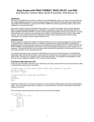
- 1. Easy Graphs with PROC FORMAT, PROC GPLOT, and ODS Apryl DeLancey, Fairbank, Maslin, Maullin & Associates, Santa Monica, CA ABSTRACT By means of straightforward commands in SAS® v8.2 and SAS/GRAPH®, graphs and charts can be generated that are visually appealing and easy to understand without having to import data into another graph-generating program. Using PROC GPLOT/GHART in conjunction with PROC FORMAT and ODS (output delivery system), data can be visualized in a comprehensible style. Many times visualizing data using traditional linear graphs or pie charts is done with a product such as Microsoft Excel or other graphing software after data is compiled and manipulated using SAS®. By using PROC GPLOT or PROC GCHART with PROC FORMAT a colorful, quality graphical representation of data can be produced. By using ODS statements, the graphs that are generated can be output to pdf (Portable Document Format) or other usable formats. The output is easily inserted into a slideshow or printed. More importantly, since the data is solely manipulated in one program, there are fewer chances for error. INTRODUCTION SAS® is capable of creating high-quality color graphics without the use of a secondary program to visualize results. In applications from academia to business, it is tempting to generate data results using SAS® and translate the graphical results in a more elementary program such as MS Excel. By using PROC CPLOT or PROC GCHART with PROC FORMAT and ODS statements, the practice of exporting SAS®-generated data into another program is not necessary. Working with the data in only one program also diminishes the possibility of introducing errors could occur from using more than on with a particular data set. The methods discussed here are intended for SAS® beginners and those with little experience in SAS/GRAPH®. Additionally, these methods will use opinion survey data as an example, but can be applied to any survey and other types of data. Generation of x*y graphs and pie charts will be described. For simplicity and accessibility for those who may not have upgraded to SAS® v9, v8.2 is used for these instances. STARTING CODE AND DATA SET At the very top of the editor, insert this code to clear the log and output screen every time and to assure that any titles or footnotes previously used are now cleared: /*CLEAR PRIOR LOG AND PRIOR OUTPUT EVERY TIME PROGRAM IS RE-RUN*/ DM LOG 'CLEAR'; DM OUTPUT 'CLEAR'; /*CLEAR EXISTING TITLES AND FOOTNOTES*/ TITLE; FOOTNOTE; RUN; Doing this minimizes error or confusion for beginners (or even seasoned SAS® experts) and makes troubleshooting easier. This is especially helpful when the program is run several times as it provides a fresh log for the last editor program that was run. For the education example described, the data set that is used will be as follows: data sample; input edu $5.0 num; cards; elem 8 hs 30 smcol 27 coll 18 postg 16 ref 1 ; run; 1
- 2. This is representative of survey data where the variable edu is educational level attained of the respondent and num is the percent of respondents that answered the corresponding level. GRAPHS AND CHARTS Generation of an x*y graph that has more than the default SAS® graph output (Figure 1) is easy with PROC GPLOT (Figure 2). Instead of using PROC PLOT to graph the education level by the percent from our data, PROC GPLOT allows for more control and visual style of the output. To choose the symbol of the data points, the following is inserted prior to the PROC GPLOT statement: symbol1 color=black value=star interpol=needle height=3 cm width=5; Where the “interpol=needle” part of the code will draw lines from the x-axis of the graph to the star (or other symbol) and produce a bar-chart look to the graph. Next, the PROC GPLOT statement: proc gplot data=sample gout=sample; plot num*edu / And to gain greater control of the axes and titles, should be followed by: haxis=axis1 vaxis=axis2 cframe=ligr; axis1 label=(height=2.0 font=swiss color=black 'Education') value=(height=1.5 font=swiss color=black); axis2 label=(height=2.0 font=swiss color=black 'Percent') value=(height=1.5 font=swiss color=black); title "Education Level Attained"; run; quit; The first line assigns what will be horizontal and vertical with respect to the axes. The code “cframe=ligr” colors in the background of the graph a light grey color. Following this are commands to format each axis. Within the “label=” parenthesis are instructions as to the height, type, and color of font – which can be adjusted. At the end of the label portion is the title of the axis. Finally, the title of the graph is given before the run statement. It is important to include “quit;” after the end of every PROC GPLOT statement. Plot of num*edu. Legend: A = 1 obs, B = 2 obs, etc. num ‚ 30 ˆ A ‚ ‚ A ‚ 25 ˆ ‚ ‚ ‚ 20 ˆ ‚ A ‚ ‚ A 15 ˆ ‚ ‚ ‚ 10 ˆ ‚ ‚ A ‚ 5 ˆ ‚ ‚ ‚ A 0 ˆ Šƒƒˆƒƒƒƒƒƒƒƒƒƒƒƒˆƒƒƒƒƒƒƒƒƒƒƒˆƒƒƒƒƒƒƒƒƒƒƒˆƒƒƒƒƒƒƒƒƒƒˆƒƒƒƒƒƒƒƒƒƒƒƒˆƒƒ coll elem hs postg ref smcol Figure 1 Education level attained by percent of respondents using PROC PLOT 2
- 3. Figure 2 Education level attained by percent of respondents using PROC GPLOT PROC FORMAT WITH PROC GHCART PROC FORMAT provides comprehensive descriptors where there are only numeric values. While this example shows political parties of respondents in a survey, it can be applied to any type of data where there are discrete responses to a survey question or medical parameter. This example uses a data set that is not given in a cards or datalines statement, but a larger SAS® data set. The first lines of the code are locating the data set: filename datafile 'data-location'; libname DataFold 'library-location'; Next, the data set used has eight discrete responses to a particular question. To make these more meaningful to the viewer, PROC FORMAT is used to give each number a label: proc format; value pty_f 1="Strong Dem" 2="NTS Dem" 3="Ind - ln Dem" 4="Independent" 5="Ind - ln Rep" 6="NTS Rep" 7="Strong Rep" 8="DTS/Other" other = " "; run; Finally, PROC GHART is used with “pie” and the “format” statement. Each slice of the pie will be a different color, with repeating colors using a different fill scheme. Also note the title1 statement to give the graph more than the standard output of “FREQUENCY OF Q27” (Figure 3): proc gchart data = datafold.procdata; pie Q27; format Q27 pty_f.; title1 'Party Self-ID'; run; quit; 3
- 4. Figure 3 Party divided into frequency ODS (OUTPUT DELIVERY SYSTEM) To have graphs or charts exported into pdf documents, the beginning of the code must have the ODS statement and then have a statement to close at the end of the code. Following is the entire code the pie chart in Figure 3 with the ODS statements that allow their export: /*PIE CHART EXAMPLE IN FIGURE 3*/ ods pdf body = "C:Aprylpie.pdf"; filename datafile 'S:220-1880procdata'; libname DataFold 'S:220-1880'; proc format; value pty_f 1="Strong Dem" 2="NTS Dem" 3="Ind - ln Dem" 4="Independent" 5="Ind - ln Rep" 6="NTS Rep" 7="Strong Rep" 8="DTS/Other" other = " "; pattern1 color=pag; pattern2 color=dagray; proc gchart data = datafold.procdata; pie Q27; format Q27 pty_f.; title1 'Party Self-ID'; run; quit; ods pdf close; Once the graphs are output, they can easily be printed out for hard-copies of presentations, or cut and pasted into presentation software, such as Microsoft PowerPoint. The ODS output could also be in HTML format by substituting “pdf” in the code for “html” at the beginning and ending ODS statements and at the extension of the resulting output. 4
- 5. CONCLUSION These methods are meant as a beginning step to producing high-quality graphics without exporting SAS® data into another graphing program. These can be expanded upon and fine-tuned to the needs of the programmer (see recommended reading). In conclusion, the methods explained here are simple and time-efficient ways to generate accurate graphs with a minimal amount of programming time. These are especially useful when the need to quickly visualize a demographic parameter or survey question. Additionally, the need to export the data to be manipulated in other graphing software can be eliminated. RECOMMENDED READING Friendly, M. http://www.psych.yorku.ca/lab/sas/ SAS Information Guides SAS® Programming Library online www.sas.com/apps/elearning modules Creating Plots, Creating Bar and Pie Charts, Enhancing and Exporting Charts and Plots, Creating Drill-Down Graphs in HTML, and Setting Graphics Options SAS Online Doc®, Version 8 http://www.csc.fi/cschelp/sovellukset/stat/sas/sasdoc/sashtml/main.htm CONTACT INFORMATION Your comments and questions are valued and encouraged. The author may be reached at: Apryl DeLancey Fairbank, Maslin, Maullin & Associates 2425 Colorado Ave Suite 180 Santa Monica, CA 90404 Work Phone: (310)828-1183 Fax: (310)453-6562 Email: apryl@fmma.com Web: fmma.com SAS and all other SAS Institute Inc. product or service names are registered trademarks or trademarks of SAS Institute Inc. in the USA and other countries. ® indicates USA registration. Other brand and product names are trademarks of their respective companies. 5