This document discusses the concept of "black swans" and economic forecasting. It begins by explaining the origin of the term "black swan" and how Nassim Taleb later used it to describe rare events with disproportionate impacts. It then discusses challenges with economic analysis and forecasting due to lack of data and uncertainties. The rest of the document focuses on analyzing past recessions and economic cycles, challenges with the recent recovery, issues around credit growth and deleveraging, and the importance of considering many interrelated factors when developing economic forecasts. It also describes the machine learning techniques and models used by the company discussed in the document to generate their economic forecasts.

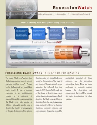
1. 1
The phrase "black swan" derives from
the Latin expression rara avis in terris
nigroque simillima cygno" - "a rare
bird in the lands and very much like a
black swan”. It was a common
expression in pre enlightenment
London as a statement of
impossibility and it was presumed that
the black swan only existed in
folklore – although it has also come to
describe the fragility of arrangements
of thought. In this use of the phrase,
the observation of a single black swan
would be the ruination of the logic of
any system of thought, as well as any
reasoning that followed from that
logic. In 2007 Nassim Taleb made use
of the phrase to describe rare events
with a disproportionate impact. Taleb
describes the black swan problem as
stemming from the use of degenerate
meta-probability. However, business
decisions, economic outcomes and
asset prices are frequently molded by
probabilistic appraisal of future
outcomes and the uncertainty
surrounding them. There are many
confounds in economic analysis
because the observation and
measurement that would be needed
for such investigations is often
wanting.
R e c e s s i o n W a t c h
DECEMBER EDITION 2014  INSIDE THIS ISSUE: THE ART OF FORECASTING - 2 • RECESSIONSIGHT - 7  PREDICTIVE STRESS TESTING - 8
F O R E S E E I N G B L A C K S W A N S T H E A R T O F F O R E C A S T I N G
© 2014 Alan Milligan

2. 2
The Great Recession of the late 2000’s, unlike most other
postwar downturns was and continues to be driven by the
extended deleveraging of the financial markets, banks
and households.
Historically the prevailing view had been that the
economic cycle reflected deviations about a trend
accredited to exogenous growth, and that the cycles were
largely comparable. However various shocks during the
1970s manifested in unexpected level and trend shifts,
forcing a reconsideration of whether the trend-stationary
archetype was the most robust model of economic
dynamics.
Statistical devices are now able to take advantage of the
increasingly computer-readable ‘big data’ environment,
such that analysis of economic fluctuations can
significantly leverage information representing an
expansive gamut of the national and international
economic system. Data from different sources and
frequencies can be scrutinized such that the
understanding of data has expanded, which permits a
richer understanding of decision making at higher
frequencies.
Models with micro-market underpinnings are now the de
facto starting point of understanding economic cycle
dynamics. Using dynamic stochastic general equilibrium
models, fiscal, monetary, preference and supply shocks
are augmented by decisions of households and firms –
influenced by cognitive biases and dissonance,
incomplete information and real and nominal
inflexibilities.
While there are distinctive similarities between
downturns, recessions that are largely a consequence of
financial market dislocations are manifestly divergent
from downturns in which financial markets participate as
submissive protagonists. Recoveries are sluggish from
financial system led downturns, specifically in the
resumption of flow of non-sovereign credit and the
reengagement of the unemployed and underemployed.
Labor share has tumbled, as has the share of
manufacturing employment. The civilian labor force
participation rate stands at 62.8 percent in November
2014, much below the peak of 67 percent in 1999. In fact,
one could posit a hypothesis that this is consistent with a
secular participation rate downtrend first established in
the year 2000. Although the female participation rate
rose from under 35 percent in 1945 to over 60 percent in
2001, the male participation rate has been relentlessly
A GLOBAL PERSPECTIVE
INTERACTIONS OF NATIONAL & TRANSNATIONAL MACRO RISK FACTORS
Fig. 2.0 Non-linear Hierarchical Clustering Analysis used in our forecasting models
©2014AlanMilligan

3. 3
falling since 1945. In addition, not only has non-
governmental indebtedness increased, but so has
indebtedness to foreign creditors. One of the most
prominent observation was the sharp reduction in
volatility of consumption, investment, and output growth
between the 1980s and the mid 2000’s, a period referred
to as the Great Moderation. However, the Great
Moderation has been supplanted by the waning of
economic activity that began just prior to the 2008 crash,
and the lack-luster recovery that followed - and to this
day is still incomplete.
The Business Cycle
A business cycle is generally understood to consist of
fluctuations in economic activity characterized by at least
two distinct states—expansionary and contractionary.
Modern mathematical inquiry of business cycles and
phases originated soon after the end of World War II,
with the pivotal work of Burns and Mitchell. They
developed a rubric to determine the phase and amplitude
of cycles after studying data on employment, production,
prices, and other macroeconomic data. The National
Bureau of Economic Research (NBER) Business Cycle
Dating Committee, the authority in dating U.S. recessions
still use their work to this day.
The NBER defines a recession as a period of falling
economic activity, real income, employment, industrial
production, and wholesale and retail sales that is
countrywide. More broadly a recession can be defined as
two consecutive quarters of decline in real GDP growth
or a 1.5 percent rise in unemployment within twelve
months. The NBER determines the interval of a recession
by the time between a peak and a trough, whilst an
expansion from trough to a peak. A complete business
cycle is defined from one trough to the next. The NBER
business cycle dates are commonly accepted as the
yardstick, even though the committee generally
announces the beginning and end of recession post-facto.
This prompts the development of methods to identify
business cycles and their turning points pre-factum.
Between the 1980s and 2008 economic growth in the
United States was steadier than at any point in the modern
historical record, with only two mild and brief recessions.
From 1945 onwards recessions were to last for a little less
than 12 months, whilst expansions averaged almost 5
years and the duration of the dozen or so business cycles
increased as a consequence of the longer expansions.
Even some sixty years ago there was an awareness of the
asymmetric price adjustment mechanism. It is now the
RECESSION & RECOVERY
Top: Credit Growth Post 2001 Recession
Bottom: Post 2008 Credit Growth vs 2001 & 1991 Recessions
ABOVE TREND
BELOW TREND
©2014AlanMilligan

4. 4
perceived wisdom that convexities
will generate asymmetric model
dynamics such that contractions are
undeniably steeper than expansions.
Markov switching models in which
the parameter values alternate
between two different states has
strong empirical evidence supporting
the hypothesis. Indeed, Markov
switching models have been
sufficiently well generalized to
permit transition probabilities to be
endogenous and to allow for a greater
number of states.
Extension to the Markov switching
model have included three-state
business cycle models (recessions,
high-growth recoveries, and mature
expansions) such that the high-
growth recovery phase can be
attributed to rapid recoveries from
recessions and firms building up
inventories in anticipation of stronger
final demand.
Widespread analysis of business
cycles frequently draws upon the
impulse-propagation framework, first
introduced in 1933 and further
elaborated during 1937. More recent
analysis has concluded that regional
and country-specific cycles co-exist
with the global business cycle and
finds that these global factors account
for significant variation in domestic
output.
Labor
From a labor perspective, recovery
from the last three recessions
manifested as slow improvements in
the employment rate, referred to as
jobless recoveries and characterized
by productivity growth rather than
increased working hours. Our Labor
Dashboard highlights some
incongruities, namely the stubborn
persistence of the underemployment
metric, below trend wage growth,
above trend mean duration of
unemployment and well below trend
labor participation rate. In fact, as of
December 2014 and by the Fed’s own
reckoning, seven of the nine labor
indicators still have not recovered to
pre-recession levels and several are
not even within the upper decile of
where they should be at this point in
time of a recovery.
Credit
The Great Recession is markedly
different from the 2001 and 1980s
recessions. In the late 1980s and 2001
recessions leverage increased
Macro Credit Dashboard
©2014AlanMilligan

5. 5
markedly just prior to the recession
followed by the broad and rapid
increase in credit during the latter
recovery phase. The recovery from
the 2008 Great Recession is really
rather unique in as much as there has
been above trend increases in both
corporate and government debt whilst
bank and households have been
embarking upon material and
sustained de-leveraging. The
unprecedented degree of bank and
shadow-financing deleveraging has
acted as a strong headwind to
recovery and many of the macro
credit indicators are substantially
below trend and someway from
where they would be expected to be
at this phase of the recovery.
The distinguishing feature of the past
three recessions is that they were not
typical of supply and demand shocks.
The recession of the early nighties
was a consequence of the savings-
and-loans crisis and the 2001 and
2008 recessions were a consequence
of monetary stimulus inflated asset
bubbles. The Great Recession of
2008 has and continues to have a
greater impact on both the broader
economy and the global economy as
housing represents a larger fraction of
household wealth than stocks and
impacts more sectors of the economy.
Financial firms have been, and
continue to deleverage at a pace
outstripping all other sectors and
agents of the economy, including
households. The roots of this can be
traced back some thirty years. The
global financial markets changed
beyond recognition in the intervening
period between the start of wholesale
deregulation in the 1980s and 2007.
In the pre deregulated world money
consisted of currency issued by the
central bank plus liabilities of private
banks in the form of deposits. Savers
provided deposits and Banks lent the
deposits to borrowers. Banks acted as
agent-intermediaries and managed
risk by judicially selecting and
monitoring borrowers while
spreading the liabilities to ensure
sustainable duration and liquidity.
Since banks were predominantly
dependent upon on short-term
liabilities to fund longer-term loans
(borrow the short-end / lend the long-
end), it was incumbent upon them to
hold a percentage of deposits as
reserves (fractional reserve system).
As a back-stop to protect taxpayers
they were also required to maintain
deposit insurance. However,
subsequent to the deregulation of the
1980s, credit was increasingly being
re-cycled through the shadow-
banking system via the use of highly
leveraged off-balance sheet
derivatives, structured credit and debt
derivatives and contingent-claim risk
transference structures. Indeed these
derivatives and synthetic debt
structures served to both obscure and
transfer the risks to more lightly
regulated parts of shadow-finance
system – both on-shore and off-shore.
Whereas 30 years ago banks made
Macro Labor Dashboard
© 2014 Alan Milligan

6. 6
loans that they held on-balance sheet,
banks were now attracted by the
favorable regulatory capital treatment
of pooled loans and asset-backed
securities, as well as new
opportunities to generate generous
fees re-packaging and selling them
onto shadow-banking clients.
Rehypothecation served to transmute
these long-dated illiquid assets into
fungible, almost as-good-as-cash
products. The purchasers of these
products were lightly regulated and
were subject to more favorable
regulatory capital treatment. This led
to a considerably extended credit
cycle that was simultaneously fanned
by central bank monetary policy (low
interest rates) and the permitted
growth of the light-touch regulated
shadow banking system. The high
leverage, low capital base of the
shadow banking system left it
exposed and vulnerable to runs - and
in late 2007 the 30 year bubble in-the-
making, finally burst.
Pro-cyclicality & Regulation
Very recent analysis has suggested
that the economic shocks are
generated in anticipation of large
financial, credit and asset shocks and
that supervisory rules and regulation
of bank risk and economic capital
requirements superimpose a pro-
cyclical component onto the
contemporaneous credit cycle. If this
is the case then one should be able to
forecast features of the economy
based upon proxies of risk and
economic capital deficiencies, or
shortfalls. Therefore it would be
prudent to include value-at-risk
(VaR), expected shortfall (ES),
trading book counterparty exposure
(PFE), recovery rate, rating transition
probabilities and credit-value-
adjustment (CVA) type
macroeconomic indicators. Indeed
when one examines the pro-cyclical
nature of post CAD-II (Basel II)
regulatory capital rules one does
observe predictive non-linear effects.
Basel III and Dodd-Frank have
introduced substantial new rule books
and changes to business conduct. This
includes mandating the use of
recognized clearing houses to clear
client over-the-counter derivatives.
CCP systemic risk is therefore a new
material risk. As a consequence we
have developed a state-of-the-art
patent pending non-linear
quantitative approach to monitoring
the risk-neutral bankruptcy risk of
CCPs. We then use this as an input
into our economic cycle forecasts as
this will likely be materially
discounted into the forward looking
anticipatory shock
Fig 3. Our CCP Risk Neutral Default Model
© 2014 Alan Milligan

7. 7
RecessionWatch has implemented machine deep
learning to analyze the following systems that influence
future economic outcomes:
 FX Microstructure Model
 Labor Model
 Credit & Liability Model
 Supply Side Model
 Demand Side Model
 Risk, Volatility & Economic Capital Model
 Relative Value Asset Model
 Global Trade and Flow Model
Each of these models makes use of information that has
been pre-conditioned using the following techniques:
 Data Transformation
 Cross Sectional Imputation
 Dimensional Reduction
 Wavelet & DFT Filtering
 ARIMAX
 GARCH Class Volatility
 Bayesian Revision Markov Blanket
 Probit & Polynomial Mixture Models
 ‘Deep’ Artificial Neural Network Ensemble
We have made good use of our expertise, knowledge &
insights gained from our real-world, living human brain
Quantitative-EEG imaging research to guide the design of
our ‘deep’ ANN ensemble. This is truly the convergence
of state-of-the-art numerical-neuroscience and artificial
neural network design.
As a result, we believe our forecasts are in a league of
their own as no other forecasting service, that we are
aware of, deploys such rigorous simulated-cognitive
forecasting methods. Picture from our quantitative electroencephalographic brain imaging product
MACHINE ‘DEEP’ LEARNING
The Machine Economist & Prop-trader

8. 8
Using the macro economic forecast
model ensemble for Reverse Stress
Testing.
An analysis conducted under
unfavourable economic scenarios
which is designed to determine
whether a bank has enough capital to
withstand the impact of adverse
developments. Stress tests can either
be carried out internally by banks as
part of their own risk management, or
by supervisory authorities as part of
their regulatory oversight of the
banking sector. These tests are meant
to detect weak spots in the banking
system at an early stage, so that
preventive action can be taken by the
banks and regulators.
Stress tests focus on a
few key risks – such as
credit risk, market risk,
and liquidity risk – to
banks' financial health
in crisis situations. The
results of stress tests
depend on the
assumptions made in
various economic
scenarios, which are
described by the
International Monetary
Fund as "unlikely but
plausible." Bank stress
tests attracted a great
deal of attention in 2009, as the worst
global financial crisis since the Great
Depression left many banks and
financial institutions severely under-
capitalized.
It is the analysis conducted under
unfavourable economic scenarios
which is designed to determine
whether a bank has enough capital to
withstand the impact of adverse
developments. Stress tests can either
be carried out internally by banks as
part of their own risk management, or
by supervisory authorities as part of
their regulatory oversight of the
banking sector. These tests are meant
to detect weak spots in the banking
system at an early stage, so that
preventive action can be taken by the
banks and regulators.
This includes:
What losses lead to dropping below a
minimum capital ratio and what
events and business lines could cause
these losses?
For a CCP, what losses could lead to
the exhaustion of one or more
defaulted member’s Initial Margin
and Default Fund Contributions?
When a financial institution should be
recapitalized under a given macro
scenario?
For a CCP, under what macro-
economic scenarios might the
guaranty fund need to be
recapitalized?
What risk factors drive the losses and
their connections with portfolio
performance?
For a CCP, this should include credit
portfolio correlations relating to
clearing member migration and
default
What are the hidden vulnerabilities of
the business model?
For a CCP, this should include
liquidity resources such as central
bank credit lines, repo facilities and
commercial bank lines
Is there any relationship between the
Stress Testing and the Reverse Stress
Testing outcomes ?
What losses lead to dropping below a
minimum capital ratio and what
events and business lines could cause
these losses?
For a CCP, what losses could lead to
the exhaustion of one or more
defaulted member’s Initial Margin
and Default Fund contributions
When a financial institution should be
recapitalized under a given macro
scenario?
S T R E S S T E S T I N G T H E U T I L I T Y O F E C O N O M I C P R E D I C T I O N

9. 9
In recent times, analyzing and
forecasting interest rate and yields has
been core for central banks, policy
makers, regulators and financial
institutions. Contemporary stochastic
term structure models fail to
reproduce important features of the
yield curve at the time horizons
required of stress testing – months to
years ahead
We propose a 4-stage approach to
modelling and stressing the interest
rate curve over long horizons.
We rationalize several features of the
data: the dynamics of the spreads
across maturities as macro-economic
conditions evolve, the relationship
between macro-economic conditions
and respective conditional variances
(ARCH process), and the relationship
between macro-economic conditions
and the respective historical records.
We proceed first by designing a
macroeconomic model that is capable
of generating future paths for the key
macroeconomic variables via a
Monte Carlo simulation, with
consideration of conditional
heteroscedasticity. The dynamics of
the interest rates will be considered
using an autoregressive structure of
the factors and also as functions of the
macroeconomic future paths
generated in the previous step. The
objective is to define a forecast model
capable of predicting the future state
of various macro-economic variables
and conditions, from 3 months to 3
years ahead.
The ARMA(3,3)-GARCH(1,1)
model explains about 86% of the
variance of the quarter ahead GDP
forecast. The application of the
GARCH model permits the
forecasting of future volatility states
via the realized volatility term
structure, and as such captures mean-
reversion, in itself counter-cyclical.
The forecasts are re-scaled at the
forecast horizon using the realized
volatility term structure imputed from
the GARCH model.
GDP year-on-year differences are
filtered by their instantaneous
conditional variance. The uncertainty
within the forecasts are explored
using numerical Monte Carlo
simulation techniques and diagnostic
challenge using ANOVA and
Regression Coefficient analysis
confirm statistical significance
(@5%)
The interest rates curve will be linked
to a set of economic factors whose
forecasts under alternative scenarios
are derived separately. The macro
model we use describes aggregate
economic activity determined by the
intersection of aggregate demand and
supply. Our model is composed of a
set of equations describing
endogenous variables. The variables
include GDP and its components,
trade, labor market, prices, and
monetary policy. The endogenous
variables are key sources of possible
exogenous shock events.
Principal Component Analysis is then
used to identify the swap curve
factors and their respective
coefficients. The factors are
elucidated through the
diagonalization of the correlation
matrix, thus they are the eigenvectors
of the data covariance matrix. The
interest rates are a linear combination
of these eigenvectors. Conditional
heteroscedasticitic filters are
calibrated and applied to the
macroeconomic differences, such that
the standard deviation equals 1.
Forecasted realized volatility term
structure is used to re-scale the
forecasted macroeconomic
standardized differences. A Monte
Carlo simulation is used to simulate
future paths, incorporating the
uncertainty within each estimator.
The objective is to calibrate a linear
model that describes changes to the
‘slope’ of the swap rate curve relative
to changes in underlying
macroeconomic variables, such as
GDP and employment.
Regression coefficient diagnostic
analysis indicates that there are 7
economic variables that explain
almost 80% of the variance of the
second principal component (‘slope’)
Analysis of the auto regression
coefficients demonstrates that there is

10. 10
statistical significance with a lag of 4,
but not with lags 1,2 or 3 with respect
to the timeseries of PC values
Review of the ANOVA analysis
indicates that the F-Value exceeds the
F-Critical at 5% significance.
The following equations describe the
mathematical relationship between
the first principal component
(‘parallel shift’), the second principal
component (‘slope’), and the
exogenous macro-economic
variables. The coefficients were
derived from the above analysis:
The forecasted macroeconomic
values in the previous slide are then
used to modulate the inputs of the
above equations, via a Monte Carlo
simulation, to derive multiple future
paths of forecasted changes in the
‘slope’ and ‘parallel’ shifts of the
swap curve. We can then take a rank
order percentile of the simulation
vectors to extract the forecasted
changes in the swap par curve at any
given confidence level at 3 months
ahead, through to 3 years ahead.
This gives us a forward (counter-
cyclical) view of possible
‘unmanageable impacts’ and ‘hidden
vulnerabilities’.
The Macro Scenarios are derived
from Bayesian inferences and
machine learned ‘knowledge’
imputed from the simulation. The
scenarios are not defined either top-
down or bottom-up via a-priori
human knowledge or expectation.
This achieves the target objective:
overcoming human behavioral
cognitive biases, such as disaster
myopia and the ‘optimism bias’
The user sets the target business
operating outcome for example,
losses that would require
recapitalization, losses that would
exceed the regulatory capital buffer,
etc and the hypothetical
macroeconomic sequence of events
leading to such outcomes would be
drawn from the simulation results
cube. Other outcomes may include:
What losses could result in us falling
below the minimum capital ratio and
what shocks, scenarios, and
businesses could precipitate this?
When should we recapitalized under
a given macroeconomic scenario?
What risk factors drive the losses and
their relationships?
What are the hidden vulnerabilities
of my business model?
Is there any relationship between the
stress testing and the reverse stress
testing outcomes?
The probability of such
macroeconomic sequences occurring
can be imputed from the simulation
results cube, such that one could
determine whether the
macroeconomic sequence was a 1-in-
20 year probability or a 1-in-5 year
probability.
Copulas have two key advantages.
Firstly, no assumptions are made
about the marginal distributions.
There is no requirement that they
should be normal distributions or that
they should have the same
distributions. The second key
advantage is the ability to separate the
dependence structure from the
marginal distributions.
These advantages allow us to describe
the same marginal distributions
through difference Copulas functions
and dependency structures. Whilst
Gaussian Copulas remain the market
standard in the same way that stock
returns are assumed to be lognormal
in the Black-Scholes model, different
Copula functions can capture
different dependency characteristics.

11. 11