Surface Wave Tomography

A Fast and Reliable Method for Surface Wave Tomography
M. P. BARMIN,1
M. H. RITZWOLLER,1
and A. L. LEVSHIN1
Abstract Ð We describe a method to invert regional or global scale surface-wave group or phase-
velocity measurements to estimate 2-D models of the distribution and strength of isotropic and azimuthally
anisotropic velocity variations. Such maps have at least two purposes in monitoring the nuclear
Comprehensive Test-Ban Treaty (CTBT): (1) They can be used as data to estimate the shear velocity of the
crust and uppermost mantle and topography on internal interfaces which are important in event location,
and (2) they can be used to estimate surface-wave travel-time correction surfaces to be used in phase-
matched ®lters designed to extract low signal-to-noise surface-wave packets.
The purpose of this paper is to describe one useful path through the large number of options available
in an inversion of surface-wave data. Our method appears to provide robust and reliable dispersion maps
on both global and regional scales. The technique we describe has a number of features that have
motivated its development and commend its use: (1) It is developed in a spherical geometry; (2) the region
of inference is de®ned by an arbitrary simple closed curve so that the method works equally well on local,
regional, or global scales; (3) spatial smoothness and model amplitude constraints can be applied
simultaneously; (4) the selection of model regularization and the smoothing parameters is highly ¯exible
which allows for the assessment of the e€ect of variations in these parameters; (5) the method allows for the
simultaneous estimation of spatial resolution and amplitude bias of the images; and (6) the method
optionally allows for the estimation of azimuthal anisotropy.
We present examples of the application of this technique to observed surface-wave group and phase
velocities globally and regionally across Eurasia and Antarctica.
Key words: Surface waves, group velocity, tomography, seismic anisotropy.
1. Introduction
We present and discuss a method to invert surface-wave dispersion measurements
(frequency-dependent group or phase velocity) on regional or global scales to
produce two-dimensional (2-D) isotropic and azimuthally anisotropic maps of
surface-wave velocities. Such ``tomographic'' maps represent a local spatial average
of the phase or group velocity at each location on the map and summarize large
volumes of surface-wave dispersion information in a form that is both useful and
easily transportable. Dispersion information in this form can be applied naturally to
a number of problems relevant to monitoring the nuclear Comprehensive Test-Ban
1
Department of Physics, University of Colorado at Boulder, Boulder, CO 80309-0390, USA.
E-mail: levshin@lemond.colorado.edu
Pure appl. geophys. 158 (2001) 1351±1375
0033 ± 4553/01/081351 ± 25 $ 1.50 + 0.20/0
Ó BirkhaÈuser Verlag, Basel, 2001
Pure and Applied Geophysics

Treaty (CTBT); For example, (1) to create phase-matched ®lters (e.g., HERRIN and
GOFORTH, 1977; RUSSELL et al., 1988; LEACH et al., 1998; LEVSHIN and RITZWOLLER,
2001, this volume) designed to detect weak surface-wave signals immersed in ambient
and signal-generated noise as a basis for spectral amplitude measurements essential
to discriminate explosions from earthquakes (e.g., STEVENS and DAY, 1985; STEVENS
and MCLAUGHLIN, 1997) and (2) in inversions to estimate the shear-velocity
structure of the crust and upper mantle (e.g., VILLASENÄ OR et al., 2001) which is useful
to improve regional event locations. The method we discuss here is designed to
produce accurate and detailed regional surface-wave maps eciently and reliably, as
well as to provide information about the quality of the maps. The method may be
applied, perhaps with a few extensions, to other 2-D inverse problems such as Pn and
Sn tomography (e.g., LEVSHIN et al., 2001).
We note, as a preface to further discussion, that the relationship between
observed seismic waveforms and an earth model is not linear. Thus, the problem of
using surface-wave data to constrain the structure of the crust and upper mantle is
nonlinear. In surface-wave inversions, however, the inverse problem is typically
divided into two parts: A nearly linear part to estimate 2-D dispersion maps and a
nonlinear part in which the dispersion maps are used to infer earth structure. It is the
nearly linear part that we call surface-wave tomography and that is the subject of this
paper. Some surface-wave inversion methods linearize the relation between the
seismic waveforms and an earth model (e.g., NOLET, 1987; SNIEDER, 1988;
MARQUERING et al., 1996) and iteratively estimate the earth model. Therefore, these
methods do not estimate dispersion maps on the way to constructing structural
models. We take the path through the dispersion maps for the following reasons.
Surface-wave dispersion maps, like a seismic model, summarize large volumes of
data in a compact form, but remain closer to the data than the models.
They are less prone to subjective decisions made during inversion and contain
fewer assumptions (both hidden and explicit).
Because of the foregoing, dispersion maps are more likely than models to be
consumed and utilized by other researchers.
Dispersion maps are directly applicable to detect and extract surface waves from
potentially noisy records, which is important in discriminating explosions from
earthquakes for CTBT monitoring.
On the negative side, dispersion maps contain only part of the information
concerning earth structure in the seismogram, are the products of inversions
themselves, and contain uncertainties due to both observational and theoretical errors.
There are a number of surface-wave tomographic techniques currently in use by
several research groups around the world. These techniques di€er in geometry (i.e.,
Cartesian versus spherical), model parameterization (e.g., global versus local basis
functions), certain theoretical assumptions (particularly about wave paths and
scattering), the regularization scheme, and whether azimuthal anisotropy can be
estimated simultaneously with the isotropic velocities. Because surface-wave tomo-
1352 M. P. Barmin et al. Pure appl. geophys.,

graphic inversions are invariably ill-posed, the regularization scheme is the focal
point of any inversion method. There is a large, general literature on ill-posed linear
or linearized inversions that applies directly to the surface-wave problem (e.g.,
TIKHONOV, 1963; BACKUS and GILBERT, 1968, 1970; FRANKLIN, 1970; AKI and
RICHARDS, 1980; TARANTOLA and VALETTE, 1982; TARANTOLA, 1987; MENKE, 1989;
PARKER, 1994; TRAMPERT, 1998). We do not intend to extend this literature, rather
the purpose of this paper is to describe one useful path through the numerous options
available to an inversion method. Our method appears to provide robust and reliable
dispersion maps on both global and regional scales.
The surface-wave tomographic method we describe here has the following
characteristics:
Geometry: Spherical;
Scale: The region of inference is de®ned by an arbitrary simple closed curve;
Parameterization: Nodes are spaced at approximately constant distances from one
another, interpolation is based on the three nearest neighbors;
Theoretical Assumptions: Surface waves are treated as rays sampling an in®nites-
imal zone along the great circle linking source and receiver, scattering is
completely ignored;
Regularization: Application of spatial smoothness (with a speci®ed correlation
length) plus model amplitude constraints, both spatially variable and adaptive,
depending on data density;
Azimuthal Anisotropy: May optionally be estimated with the isotropic velocities.
The theoretical assumptions that we make are common in most of surface-wave
seismology. The method we describe generalizes naturally to non-great circular
paths, if they are known, with ®nite extended Fresnel zones (e.g., PULLIAM and
SNIEDER, 1998). The incorporation of these generalizations into surface-wave
tomographic methods is an area of active research at this time. The use of the
scattered wave®eld (the surface wave coda) is also an area of active research (e.g.,
POLLITZ, 1994; FRIEDERICH, 1998), but usually occurs within the context of the
production of a 3-D model rather than 2-D dispersion maps.
The choices of parameterization and regularization require further comment.
1.1. Parameterization
There are four common types of basis functions used to parameterize velocities in
surface-wave tomography: (1) Integral kernels (the Backus-Gilbert approach), (2) a
truncated basis (e.g., polynomial, wavelet, or spectral basis functions), (3) blocks,
and (4) nodes (e.g., TARANTOLA and NERSESSIAN, 1984). In each of these cases, the
tomographic model is represented by a ®nite number of unknowns. Blocks and nodes
are local whereas wavelets and polynomials are global basis functions. (To the best of
our knowledge, wavelets have not yet been used in surface-wave tomography.)
Backus-Gilbert kernels are typically intermediary between these extremes. Blocks are
Vol. 158, 2001 A Method for Surface Wave Tomography 1353

2-D objects of arbitrary shape with constant velocities and are typically packed
densely in the region of study. They are typically regularly shaped or sized, although
there are notable exceptions (e.g., SPAKMAN and BIJWAARD, 1998, 2001). Nodes are
discrete spatial points, not regions. A nodal model is therefore de®ned at a ®nite
number of discrete points and values in the intervening spaces are determined by a
speci®c interpolation algorithm in the inversion matrix and travel-time accumulation
codes. Nodes are not necessarily spaced regularly. The ability to adapt the
characteristics of these basis functions to the data distribution and other a priori
information is a desirable characteristic of any parameterization, and is typically
easier with local than with global basis functions. Blocks can be thought of as nodes
with a particularly simple interpolation scheme. Thus we use nodes rather than
blocks because of their greater generality.
To date, most surface-wave travel time tomographic methods have been designed
for global application and have utilized truncated spherical harmonics or 2-D
B-splines as basis functions to represent the velocity distribution (e.g., NAKANISHI
and ANDERSON, 1982; MONTAGNER and TANIMOTO, 1991; TRAMPERT and WOOD-
HOUSE, 1995, 1996; EKSTROÈ M et al., 1997; LASKE and MASTERS, 1996; ZHANG and
LAY, 1996). There are two notable exceptions. The ®rst is the work of DITMAR and
YANOVSKAYA (1987) and YANOVSKAYA and DITMAR (1990) who developed a 2-D
Backus-Gilbert approach utilizing ®rst-spatial gradient smoothness constraints for
regional application. This method has been extensively used in group velocity
tomography (e.g., LEVSHIN et al., 1989; WU and LEVSHIN, 1994; WU et al., 1997;
RITZWOLLER and LEVSHIN, 1998; RITZWOLLER et al., 1998; VDOVIN et al., 1999) for
studies at local and continental scales. The main problem is that the method has been
developed in Cartesian coordinates, and sphericity is approximated by an inexact
earth ¯attening transformation (YANOVSKAYA, 1982; JOBERT and JOBERT, 1983)
which works well only if the region of study is suciently small (roughly less than
one-tenth of the earth's surface). YANOVSKAYA and ANTONOVA (2000) recently
extended the method to a spherical geometry, however. The second is the irregular
block method of SPAKMAN and BIJWAARD (2001).
We prefer local to global basis functions due to the simplicity of applying local
damping constraints, the ability to estimate regions of completely general shape and
size, and the ease by which one can intermix regions with di€erent grid spacings. For
example, with local basis functions it is straightforward to allow damping to vary
spatially, but it is considerably harder to target damping spatially with global basis
functions. This spatially targeted damping is a highly desirable feature, particularly if
data distribution is inhomogeneous.
1.2. Regularization
The term `regularization', as we use it, refers to constraints placed explicitly on the
estimated model during inversion. These constraints appear in the ``penalty function''

that is explicitly minimized in the inversion. We prefer this term to `damping' but take
the terms to be roughly synonymous and will use them interchangeably. Regular-
ization commonly involves the application of some combination of constraints on
model amplitude, the magnitude of the perturbation from a reference state, and on
the amplitude of the ®rst and/or second spatial gradients of the model. It is typically
the way in which a priori information about the estimated model is applied and
how the e€ects of inversion instabilities are minimized. The strength of regularization
or damping is usually something speci®ed by the user of a tomographic code, but may
vary in an adaptive way with information regarding data quantity, quality, and
distribution and relating to the reliability of the reference model or other a priori
information. As alluded to above, the practical di€erence between local and global
basis functions manifests itself in how regularization constraints (e.g., smoothness)
are applied as well as the physical meaning of these constraints.
As described in section 2, the regularization scheme that we have e€ected involves
a penalty function composed of a spatial smoothing function with a user-de®ned
correlation length and a spatially variable constraint on the amplitude of the
perturbation from a reference state. The weight of each component of the penalty
function is user speci®ed, but the total strength of the model norm constraint varies
with path density. Our experience indicates that Laplacian or Gaussian smoothing
methods are preferable to gradient smoothing methods. The ®rst-spatial gradient
attempts to produce models that are locally ¯at, not smooth or of small amplitude.
This works well if data are homogeneously distributed, but tends to extend large
amplitude features into regions with poor data coverage and con¯icts with amplitude
penalties if applied simultaneously. The model amplitude constraint smoothly blends
the estimated model into a background reference in regions of low data density such
as the areas on the fringe of the region under study. In such areas the path density is
very low, and the velocity perturbations will be automatically overdamped due to
amplitude constraints. The dependence on data density is also user speci®ed.
2. Surface-wave Tomography
Using ray theory, the forward problem for surface-wave tomography consists of
predicting a frequency-dependent travel time, tR=L…x†, for both Rayleigh (R) and
Love (L) waves from a set of 2-D phase or group velocity maps, c…r; x†:
tR=L…x† ˆ

p
cÀ1
R=L…r; x†ds ; …1†
where r ˆ ‰h; /Š is the surface position vector, h and / are colatitude and longitude,
and p speci®es the wave path. The dispersion maps are nonlinearly related to the
seismic structure of the earth, M…r; z†, where for simplicity of presentation we have
assumed isotropy, and M…r; z† ˆ ‰vs…z†; vp…z†; q…z†Š…r† is the position dependent

structure vector composed of the shear and compressional velocities and density.
Henceforth, we drop the R=L subscript and, for the purposes of discussion here, do not
explicitly discriminate between group and phase velocities or their integral kernels.
By surface-wave tomography we mean the use of a set of observed travel times
tobs
…x† for many di€erent paths p to infer a group or phase velocity map, c…r†, at
frequency x. We assume that
tobs
…x† ˆ t…x† ‡ …x† ;
where is an observational error for a given path. The problem is linear if the paths p
are known. Fermat's Principle states that the travel time of a ray is stationary with
respect to small changes in the ray location. Thus, the wave path will approximate
that of a spherically symmetric model, which is a great-circle linking source and
receiver. This approximation will be successful if the magnitude of lateral
heterogeneity in the dispersion maps is small enough to produce path perturbations
smaller than the desired resolution.
2.1. The Forward Problem
Because surface-wave travel times are inversely related to velocities, we
manipulate equation (1) as follows. Using a 2-D reference map, c…r†, the travel-
time perturbation relative to the prediction from c…r† is:
dt ˆ t À t ˆ

p
ds
c
À

p
ds
c
ˆ

p
m
c
ds …2†
m ˆ
c À c
c
; …3†
where we have suppressed the r ˆ ‰h; /Š dependence throughout and have assumed
that the ray-paths are known and are identical for both c and c.
For an anisotropic solid with a vertical axis of symmetry, the surface-wave
velocities depend on the location r and the local azimuth w of the ray. In the case of a
slightly anisotropic medium, SMITH and DAHLEN (1973) show that phase or group
velocities can be approximated as:
c…r† ˆ cI …r† ‡ cA…r† …4†
cI …r† ˆ A0…r† …5†
cA…r† ˆ A1…r† cos…2w† ‡ A2…r† sin…2w†
‡ A3…r† cos…4w† ‡ A4…r† sin…4w† ; …6†
where cI is the isotropic part of velocity, cA is the anisotropic part, A0 is the isotropic
coecient, and A1; . . . ; A4 are anisotropic coecients. If we assume that jcA=cI j ( 1
so that …1 ‡ cA=cI †À1
% …1 À cA=cI †, and if the reference model c is purely isotropic,
then by substituting equations (4)±(6) into (3) we get:

m %
c À cI
cI
À
cA
cI
À
cA
cI

c À c
cI

%
c À cI
cI
À
cA
c2
I
c ;
…7†
where the latter equality holds if jcA=cI j ( 1 as before. Equation (7) can be rewritten
as:
m…r; w† ˆ
ˆn
kˆ0
ck…w†mk…r† ; …8†
where n should be 0, 2 or 4 for a purely isotropic model, a 2w anisotropic model, or a
4w anisotropic model, respectively, and ck and mk are de®ned as follows:
c0…w† ˆ 1 m0…r† ˆ c…r† À cI …r†… †=cI …r†
c1…w† ˆ À cos…2w† m1…r† ˆ A1…r†c…r†=c2
I …r†
c2…w† ˆ À sin…2w† m2…r† ˆ A2…r†c…r†=c2
I …r†
c3…w† ˆ À cos…4w† m3…r† ˆ A3…r†c…r†=c2
I …r†
c4…w† ˆ À sin…4w† m4…r† ˆ A4…r†c…r†=c2
I …r† :
…9†
2.2. The Inverse Problem
Our goal is to estimate the vector function m…r† ˆ ‰m0…r†; . . . ; mn…r†Š using a set of
observed travel-time residuals d relative to the reference model c…r†:
d ˆ dtobs
ˆ tobs
À t ˆ

p
m
c
ds ‡ : …10†
From m…r† we can reconstruct cI ; A1; . . . ; A4 for substitution into equations (4)±(6):
cI ˆ
c
1 ‡ m0
…11†
Ak ˆ
mk
1 ‡ m0
cI …k Tˆ 0† : …12†
We de®ne the linear functionals Gi as:
Gi…m† ˆ
ˆn
kˆ0

pi
ck w…r†… †cÀ1
…r†
À Á
mk…r†ds : …13†
By substituting equations (8) and (13) into equation (10) for each path index
…1 i N† we obtain the following:

di ˆ dtobs
i ˆ Gi…m† ‡ i : …14†
To estimate m we choose to minimize the following penalty function:
…G…m† À d†T
CÀ1
…G…m† À d† ‡
ˆn
kˆ0
a2
kjjFk…m†jj2
‡
ˆn
kˆ0
b2
kjjHk…m†jj2
; …15†
where G is a vector of the functionals Gi. For an arbitrary function f …r† the norm is
de®ned as: jj f …r†jj2
ˆ
‚
S f 2
…r† dr.
The ®rst term of the penalty function represents data mis®t (C is the a priori
covariance matrix of observational errors i). The second term is the spatial
smoothing condition such that
Fk…m† ˆ mk…r† À

S
Sk…r; rH
†mk…rH
†drH
; …16†
where Sk is a smoothing kernel de®ned as follows:
Sk…r; rH
† ˆ K0k exp À
jr À rH
j2
2r2
k
2 3
…17†

S
Sk…r; rH
† drH
ˆ 1 ; …18†
and rk is spatial smoothing width or correlation length. The minimization of the
expression in equation (16) explicitly ensures that the estimated model will
approximate a smoothed version of the model.
The ®nal term in the penalty function penalizes the weighted norm of the model,
Hk…m† ˆ H…q…r†; v…r††mk ; …19†
where H is a weighting function that depends on local path density q for isotropic
structure and a measure of local azimuthal distribution v for azimuthal anisotropy.
Thus, for k ˆ 0, H ˆ H…q† and for k ˆ 1; . . . ; 4, H ˆ H…v†. Path density is de®ned
as the number of paths intersecting a circle of ®xed radius with center at the point r.
For isotropic structure we choose H to approach zero where path density is suitably
high and unity in areas of poor path coverage. The function H…q† can be chosen in
various ways. We use H ˆ exp…Àkq†, where k is a user-de®ned constant. An example
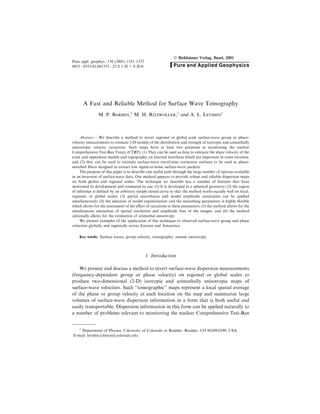
is shown in Figure 1. To damp azimuthal anisotropy in regions with poor azimuthal
coverage, we de®ne v…h; /† to measure the azimuthal distribution of ray paths at
point …h; /†. To ®nd v we construct a histogram of azimuthal distribution of raypaths
in the vicinity of …h; /† for a ®xed number n of azimuthal bins in the interval between
0
and 180
, and evaluate the function

v ˆ
€n
iˆ1
fi
n max
i
fi
; …20†
where fi is the density of azimuths in the ith bin. Values of v are in the range
1=n v 1. v % 1 characterizes an almost uniform distribution of azimuths, and
v % 1=n is an indicator of the predominance of a single azimuthal direction (large
azimuthal gap). We assume that the anisotropic coecients cannot be determined
reliably in regions where v is less than $ 0:3. Examples of a v map and the histogram
of azimuthal density, f …w†, are given in Section 3.4 (Figs. 8c,d).
Because m is a perturbation from a reference state, the e€ect of the third term
in the penalty function is to merge the estimated model smoothly and
continuously into the isotropic reference state in regions of poor data coverage.
In regions of good coverage, this term has no e€ect so that the only
regularization is the smoothness constraint represented by the second term in
expression (15).
The user-supplied regularization constants, ak and bk, de®ne the relative
strengths of the three terms in the penalty function. The smoothing width or
correlation length rk is also speci®ed by the user. These parameters should be
varied systematically in applying the method. In practice, we often estimate the
isotropic and anisotropic maps simultaneously. In this case we normally use slightly
di€erent values of all three constants ak, bk, rk for the isotropic and anisotropic
maps to make anisotropic maps more smooth. Typically a1 ˆ a2 and a3 ˆ a4, r1=
r2, r3= r4, and bk ˆ b.
0.0
0.2
0.4
0.6
0.8
1.0
DampingFactorH(ρ)
0 10 20 30 40
Path Density ρ
Figure 1
Example of the model norm weighting function, H…q† that we commonly use; e.g., as Figure 5. Here we
choose the constant k $ 0:147 so that when path density (q) is less than about 20 paths per 50,000 km2
damping toward the input reference model becomes increasingly strong.

2.3. Discretization
The discretization of the equations in the preceding section involves two steps: (1)
the formation of a discrete grid and the evaluation of the model on this grid and (2)
the discretization of the penalty function. We discuss each in turn.
2.3a. Grid, Nearest Neighbors, and Interpolation
The goal is to generate a discrete grid with nodes that are approximately
constantly spaced on a sphere such that nearest neighbors can be identi®ed and the
model evaluated at these points quickly. Signi®cant advances in nonconstant grid
generation have been made in recent years by several researchers (e.g., SAMBRIDGE
et al., 1995; SPAKMAN and BIJWAARD, 1998), particularly for application in 3-D
body-wave tomography. The tomographic method that we describe is applicable
irrespective of grid. However, because path coverage for regional surface waves tends
to be less variable than for body waves, and surface-wave tomography is only in 2-D
(e.g., BIJWAARD et al., 1998; VAN DER HILST et al., 1997; GRAND et al., 1997; ZHOU,
1996), we ®nd that a constant grid is sucient for our purposes. Generalization to
nonconstant grids for surface wave tomography is, however, a useful direction for
future research (e.g., SPAKMAN and BIJWAARD, 2001).
We create a nearly constant grid on a sphere by performing a central projection
onto the sphere of a grid on a reference cube, such that the cube and the sphere share
a common center. The advantage of using this reference cube is that nearest
neighbors on each of the six faces of the cube are identi®ed trivially. Ecient
neighbor identi®cation for interpolation during model evaluation is important for
travel-time accumulation, which occurs during the construction of the inversion
matrix, and in the application of the smoothness constraint. Thus, this method is
computationally very ecient because it imposes a natural ordering for the nodes on
the sphere, which avoids the need for the creation and use of an adjacency matrix
(e.g., SLOAN, 1987; SAMBRIDGE et al., 1995). To ensure that the distances between
nodes on the sphere are approximately constant, the grid on the reference cube must
be non-constant. Without providing the details, Figure 2 demonstrates the mapping
between the face of a cube and the spherical shell related to the face. The current
method of grid generation guarantees that the areas de®ned by adjacent quadruples
of nodes on the sphere di€er by no more than 10% from the average area. One could
produce a mapping with smaller variation in these areas, but this is good enough for
our purposes.
The value of the model at each location on the sphere is evaluated from the values
at the three nearest nodes. This is done by constructing Delaunay triangles from the
set of nodes on the sphere (e.g., AURENHAMMER, 1991; BRAUN and SAMBRIDGE,
1997). Each triangle de®nes a ¯at plane between the three nodes at the vertices on the
plane which is nearly the tangent plane to the sphere. We de®ne a local Cartesian
coordinate system on this plane and determine the distances between the point of

interest and the three de®ning nodes approximately. Typical internodal distances,
even for global inversions, are 200 km or less, therefore this local Cartesian
approximation is accurate enough for our purposes. Three-point linear interpolation
is used to evaluate the model within each Delaunay triangle. Thus, the value of the
model at some arbitrary point r can be expressed as the weighted sum of the values at
the three neighboring nodes:
mk…r† ˆ
ˆM
jˆ1
mk…rj†wj…r† ; …21†
where rj are the locations of the M nodes (vortices of triangles) de®ning the model.
The weights wj…r† are non-zero only inside the triangles surrounding rj and linearly
depend on two local coordinates inside the Delaunay triangle enclosing r. The
weights wj…r† form the set of the local basis functions such that the values of the basis
functions range from 0 to 1 with a maximum value of 1 at the point rj.
2.3b. The Inversion Matrix
To construct the inversion matrix we must substitute equation (21) into
expression (15). After integrating, the penalty function can be rewritten in matrix
form as the sum of two quadratic forms,
Gm À d… †T
CÀ1
Gm À d… † ‡ mT
Qm ; …22†
in which the second term is the regularization condition that includes both
smoothness and model norm constraints. Let N be the number of data, n be the
Figure 2
An example of the Delaunay triangulation on a sphere by de®ning a variable triangular grid on a reference
cube and performing a central projection of the grid onto the sphere.

isotropic/anisotropic index (0 for isotropic, 2 for isotropic plus 2w anisotropic, 4 for
isotropic plus both 2w and 4w anisotropic), and M be the number of nodes de®ning
the model such that k ˆ 0; . . . ; n, i ˆ 1; . . . ; N, j ˆ 1; . . . ; M.
Let us de®ne now our discrete model as a vector m in the following way:
m ˆ …m0…r1†; m0…r2†; . . . ; m0…rM †; . . . ; mn…r1†; mn…r2†; . . . ; mn…rM ††T
:
Without changing notation we discretize G to create a N Â …n ‡ 1†M matrix in the
following way. Let G be composed of a set of n submatrices, Uk
,
G ˆ U0
Â Ã
…n ˆ 0†
G ˆ U0..
.
U1..
.
U2
!
…n ˆ 2†
G ˆ U0..
.
U1..
.
U2..
.
U3..
.
U4
!
…n ˆ 4†
…23†
where Uk
is de®ned as follows:
Uk
ij ˆ

pi
ck w… †cÀ1
0 …r†
À Á
wj r… †ds : …24†
The …n ‡ 1†M Â …n ‡ 1†M regularization matrix Q is the result of discrete
numerical integration of the last two terms in equation (15), and can be determined
in the following way:
Q ˆ FT
F ‡ HT
H ; …25†
where the smoothing constraint is incorporated within the …n ‡ 1†M Â …n ‡ 1†M
block-diagonal matrix F as follows:
F ˆ
a0F0
. . . 0 . . . 0
..
. ..
. ..
. ..
. ..
.
0 . . . akFk
. . . 0
..
. ..
. ..
. ..
.
0
0 . . . 0 . . . anFn
P
T
T
T
T
T
T
R
Q
U
U
U
U
U
U
S
: …26†
The M Â M matrices Fk
ˆ F k
jjH

(k ˆ 0; . . . ; n; j; jH
ˆ 1; . . . ; M) are:
F k
jjH ˆ
1 j ˆ jH
ÀSk…rj; rjH †=pk j Tˆ jH
,

pk ˆ
ˆ
jH
Sk…rj; rjH † : …27†
The model norm constraint is encoded within the …n ‡ 1†M Â …n ‡ 1†M matrix H
which consists of …n ‡ 1† diagonal matrices Hk
ˆ Hk
jjH

:

H ˆ
b0H0
. . . 0 . . . 0
..
. ..
. ..
. ..
. ..
.
0 . . . bkHk
. . . 0
..
. ..
. ..
. ..
. ..
.
0 . . . 0 . . . bnHn
P
T
T
T
T
T
T
R
Q
U
U
U
U
U
U
S
…28†
where
Hk
jjH ˆ
H q…rj†; v…rj†
À Á
j ˆ jH
0 j Tˆ jH
.

…29†
With these de®nitions the forward problem for the travel-time perturbation
relative to an isotropic reference model is:
dt ˆ Gm ; …30†
and the estimated model is:
^m ˆ Gy
CÀ1
dt …31†
where the inversion operator, Gy
, is de®ned as follows:
Gy
ˆ GT
CÀ1
G ‡ Q
À ÁÀ1
GT
: …32†
2.4. Resolution Analysis
We agree with LEVEQUE et al. (1993) who argue that the estimation of the
resolution matrix is generally preferable to checkerboard tests such as those
performed by RITZWOLLER and LEVSHIN (1998). Note that from equations (30)±
(32):
^m ˆ Gy
CÀ1
dt ˆ Gy
CÀ1
G
À Á
m ˆ Rm …33†
R ˆ GT
CÀ1
G ‡ Q
À ÁÀ1
GT
CÀ1
G : …34†
The matrix R is the resolution matrix. In this application each row of R is a
resolution map de®ning the resolution at one spatial node. Thus, the resolution
matrix is very large and the information it contains is somewhat dicult to utilize.
We attempt to summarize the information in each resolution map by estimating two
scalar quantities at each point: spatial resolution and amplitude bias.
To estimate spatial resolution we ®t a cone to each resolution map. This cone
approximates closely the response of the tomographic procedure to a d-like
perturbation at the target node. Figure 3a shows a d-like input perturbation (the
local basic function) at the speci®ed spatial location. Figure 3b displays the
resolution map for that spatial location for the 50 s Rayleigh wave. The cone that

best ®ts the resolution surface for this point is shown in Figure 3c and the di€erence
between the ®t cone and the resolution map appears in Figure 3d. We de®ne the
resolution rR as the radius of the base of the ®t cone. This value may be interpreted
as the minimum distance at which two d-shaped input anomalies (i.e., Fig. 3a) can be
resolved on a tomographic map. Of course, resolution cannot be less than 2`, where `
is the distance between the nodes. In the example in Figure 3, nodes are separated by
2 equatorial degrees ($222 km). Therefore, if rR is estimated to be less than 2` or
444 km, we rede®ne resolution as rR ˆ 2` ˆ 444 km.
It is also useful to know how reliably the amplitude of the estimated anomalies
may be determined. To do this we apply the appropriate row of the resolution matrix
(eq. 33) associated with node (h0; /0) to a test model consisting of a cylinder of unit
height with a diameter equal to 2rR centered at (h0; /0). We then de®ne the amplitude
65
70
75
80
Longitude
35
40
45
50
Latitude
0.00.20.40.60.81.0
Amplitude
0.00.20.40.60.81.0
Amplitude a
65
70
75
80
Longitude
35
40
45
50
Latitude
0.00.10.20.3
Amplitude
0.00.10.20.3
Amplitude
b65
70
75
80
Longitude
35
40
45
50
Latitude
0.00.10.20.3
Amplitude
0.00.10.20.3
Amplitude
c
65
70
75
80
Longitude
35
40
45
50
Latitude
-0.10.00.10.2
Amplitude
-0.10.00.10.2
Amplitude
d
Figure 3
Graphical description of the resolution analysis. (a) Minimum sized function that can be estimated with a
2
Â 2
grid. The function is centered at 42
N latitude and 73
E longitude. (b) The row of the resolution
matrix (a resolution map) for the point speci®ed in (a) for the 50 s Rayleigh wave. (c) The cone that best ®ts
the row of the resolution matrix shown in (b). A comparison of (a) with (b) and (c) demonstrates the spatial
spreading produced in the tomographic procedure. (d) The di€erence between the resolution map and the
best-®tting cone.

of the ®t surface as the average amplitude within rR of the center of the input
cylinder. The relative di€erence between the input and estimated amplitudes is then
taken as the amplitude bias estimate for this point on the map.
Examples of the estimated resolution and amplitude bias are shown in Figure 4
for the 20 s Rayleigh wave. Across much of Eurasia the 20 s Rayleigh wave data
yields nearly optimal resolution for a 2
Â 2
grid spacing; about 450 km. Amplitude
bias at the estimated resolution is typically within about Æ10% at each spatial point.
Near the periphery of the map where data coverage degrades, estimates of spatial
resolution become unreliable but amplitude bias grows rapidly. Thus, amplitude bias
is a more reliable means of estimating the reliability of dispersion maps in regions of
extremely poor data coverage, using the method we describe here.
2.5. Computational Requirements
The following formulas summarize computational time (550 MHz, DEC Alpha)
and memory requirements for a purely isotropic inversion:
t $ 68
k
d
4
hours (computational time in hours) …35†
450 500 550 600 650 700 1000 2000
a
Resolution (km)
-10 -5 -2 2 5 10 15 25 50 75 100
b
Amplitude Bias (%)
Figure 4
(a) Spatial resolution in km for the 20 s Rayleigh wave across Eurasia. Resolution depends on data
coverage. In the central part of Eurasia the resolution is high ($ 450±500 km) in areas of high path density
and degrades rapidly on the periphery of the region where path density (Fig. 5d) is low. (b) Amplitude bias
for Rayleigh waves at 20 s period. Units of amplitude bias are percent such that 0% means that the
cylindrical test function's amplitude has been fully recovered upon inversion. Amplitude bias across the
region varies between about Æ10% depending on path coverage.

M $ 29
k
d
4
Gb (memory usage in Gb) ; …36†
where k is the fraction of the earth's surface covered and d is the distance between
nodesf in equatorial degrees. For Eurasian tomography about half of the earth's
surface is covered (k $ 0:5) and d ˆ 2 degrees = 222 km, thus t $ 15 minutes and
M $ 115 Mb.
3. Examples of Applications
3.1. Preliminaries
The technique described above has been extensively tested using di€erent cell
sizes, regularization parameters, and data sets from di€erent regions of the world:
Eurasia, Antarctica, South America, and the Arctic. The two conditions necessary
for constructing reliable tomographic images are preliminary outlier rejection (data
``cleaning'') and a careful choice of regularization (or damping) parameters
appropriate for a given path coverage.
Data cleaning is based on a two part process. First, we identify outliers in a
preliminary way by clustering measurements into summary rays. Second, the
resulting data are inverted for an overdamped, smooth tomographic map and
outliers are then identi®ed by comparing observed group travel times with those
predicted from the smooth map. The usual percentage of the rejected measurements
is about 2±3% of all observations.
The choice of regularization parameters is made after several iterations using
di€erent combinations of the parameters ak, bk, rk. The criteria for choosing the best
combination are subjective and are based on common sense and some a priori
information regarding the region under study. We select a combination of
parameters that produces a map free from aphysical features like speckling,
streaking, and other artifacts and that also reveals the well known features of the
region (sedimentary basins, mountain ranges, etc.) appropriate for the type of map
under construction. RITZWOLLER and LEVSHIN (1998) describe this procedure in
detail. For example, a typical combination of parameters selected for an isotropic
inversion of the 20 s Rayleigh wave data for Eurasia on a 2
Â 2
grid is: a0 ˆ 800,
b0 ˆ 1, and r0 ˆ 200. The resulting maps are relatively insensitive to small (20±30%)
changes in the damping parameters. Similar robustness of maps of azimuthal
anisotropy to changes in the anisotropy damping parameters was demonstrated by
VDOVIN (1999) for Antarctica, but in other areas of the world both the pattern and
the amplitude of anisotropy change strongly with damping (e.g., Eurasia and the
Arctic, LEVSHIN et al., 2001) as discussed further in section 3.4.

3.2. Regional Isotropic Group-velocity Maps
Regional group- and phase-velocity maps have been produced by a number of
researchers (e.g., SUETSUGU and NAKANISHI, 1985; CURTIS et al., 1998; RITZWOLLER
et al., 1999; and many others). Using the protocol described in section 3.1, we have
recently constructed a set of isotropic group velocity maps of Eurasia and
surrounding areas for Rayleigh and Love waves from 15 s to 200 s period. An
example for the 20 s Rayleigh wave is shown in Figure 5a. As input data we used
12900 Rayleigh group velocity measurements obtained from records of both global
(GSN, GEOSCOPE) and regional (CDSN, CSN, USNSN, MEDNET, Kirgiz and
Kazak networks) networks. The basic characteristics of the measurement procedure,
data control and weighting are described in detail in RITZWOLLER and LEVSHIN
(1998). Because 20 s Rayleigh waves are most sensitive to upper crustal velocities, the
corresponding group velocity map clearly shows the signi®cant sedimentary basins
across Eurasia and on the periphery of the Arctic Ocean as low velocity anomalies
(e.g., Barents Sea shelf, western Siberian sedimentary complex, Pre-Caspian, South
Caspian, Black Sea, Tadzhik Depression, the Tarim Basin, Dzhungarian Basin,
Ganges Fan and Delta, etc.) There is qualitative agreement between the observed
group velocity map and the prediction of a hybrid model composed of crustal
structure from the model CRUST5.1 (MOONEY et al., 1998) and mantle velocities
from the model S16B30 (MASTERS et al., 1996). The comparison is shown in Figures
5b,c. The estimated r.m.s. group velocity mis®t at 20 s period is signi®cantly less for
our maps (0.08 km/s) than for the map computed from the model CRUST5.1/
S16B30 (0.14 km/s). The numbers for the 50 s Rayleigh wave are correspondingly
0.05 km/s and 0.16 km/s. Similar results are reported by RITZWOLLER and LEVSHIN
(1998) which used the tomographic method of DITMAR and YANOVSKAYA (1987).
Figure 6 presents group travel-time correction surfaces for the 40 s Rayleigh wave
for several stations in Central Asia. These surfaces summarize travel-time informa-
tion in group velocity maps to be used to improve detection and discrimination
schemes in nuclear monitoring (LEVSHIN and RITZWOLLER, 2001, this volume).
LEVSHIN and RITZWOLLER (2001) also present an example of travel-time correction
surfaces for the 20 s Rayleigh waves.
3.3. Global Isotropic Phase-velocity Maps
The tomographic method described above identi®es the region of interest by
requiring the user to de®ne a simple closed curve on the sphere and identify a single
point outside the contour that distinguishes the inside from the outside of the region
of interest. If the contour is a very small circle surrounding the point, then the region
of interest becomes nearly the entire sphere. In this way, our method can be used to
produce global tomographic maps on a regular grid. An example is shown in Figure
7a, in which we have inverted the 100 s Rayleigh wave phase velocity data of
TRAMPERT and WOODHOUSE (1995, 1996). Trampert and Woodhouse's map is shown

-28 -12 -9 -6 -4 -2 2 4 6 9 12 37
a
δU/U (%)
-28 -12 -9 -6 -4 -2 2 4 6 9 12 37
δU/U (%)
b
-28 -12 -9 -6 -4 -2 2 4 6 9 12 37
δU/U (%)
c
0 10 20 40 60 100 150 250 430
d
Path Density
Figure 5
(a) The group-velocity map across Eurasia for the 20 s Rayleigh wave using the method described in this
paper. A 2
Â 2
grid is used. (b) The group-velocity map computed from the smoothed version of the
model CRUST5.1/S16B30. Maps (a) and (b) are plotted in percent relative to the same average velocity. (c)
The di€erence between maps (a) and (b) relative to the same average in (a) and (b). (d) Path density,
de®ned as the number of rays intersecting a 2
square cell ($50,000 km2
). White lines are plate boundaries.
The red lines delineate the contour of 20 paths per 50,000 km2
. Inside this contour we have the greatest
con®dence in the estimated maps. Outside it, model norm damping begins to take e€ect.

in Figure 7b, where they used spherical harmonics up through degree and order 40.
The major features of these maps are nearly identical. We have chosen the damping
parameters, however, to accentuate smaller scale features than those apparent in the
spherical harmonic parameterization. There is considerable signal remaining in the
data set of Trampert and Woodhouse to be ®t by smaller scale features than those
apparent in Figure 7b. For example, the rms mis®t to Trampert and Woodhouse's
data produced by the map in Figure 7a is about 8.1 s compared with the 10.8 s
produced by the spherical harmonic map in Figure 7b; about a 40% reduction in
variance.
3.4. Azimuthal Anisotropy
We follow the majority of the studies of azimuthal anisotropy and our
discussion above (equations (4)±(6)) by parameterizing azimuthal anisotropy for
group velocity as:
60E 90E
15N
30N
45N
60N
-305
-195
-85
25
135
245
30E
60E
90E
15N
30N
45N
60N
-470
-320
-170
-20
130
300
30E
60E 90E
30N
45N
60N
75N
-385
-280
-180
-80
20
140
60E
90E 120E
30N
45N
60N
75N
-325
-200
-75
50
175
300
TLY
BRVK
ABKT
AAK
(m/s)
Group Velocity Correction Surfaces
40 s Rayleigh Wave
Figure 6
Group velocity correction surfaces for four stations in Central and Southern Asia for the 40 s Rayleigh
wave. For each geographical point the maps de®ne the group velocity perturbation that should be applied
to a 40 s Rayleigh wave observed at a station if an event were located at the chosen point. Perturbations
are relative to the group velocity at the station. Units are m/s. The locations of the Chinese and Indian test
sites are indicated with stars.

U…r; w† ˆ U0…r† ‡ U1…r† cos 2w ‡ U2…r† sin 2w ‡ U3…r† cos 4w ‡ U4…r† sin 4w ; …37†
where U0 is isotropic group velocity at spatial point r ˆ …h; /†, U1 and U2 de®ne the
2w part of azimuthal anisotropy, and U3 and U4 the 4w part of azimuthal anisotropy.
Figure 8 presents examples of the 2w component of group velocity azimuthal
anisotropy for the 50 s Rayleigh wave across Antarctica and the surrounding oceans.
We took the approximately 2200 observations and divided them into two separate
sets of about 1100 measurements each which we then inverted separately for the two
maps in Figures 8a,b. Both maps display spatially smooth anisotropy patterns, and
the fast axes at many locations tend to be parallel to the directions of plate motions.
The main features of the maps are similar, but there are di€erences in detail. In order
to quantify the correlation between these two 2w maps we use the coherence function
de®ned by GRIOT et al. (1998) which takes into account di€erences in the fast axes
directions …a1…h; /†; a2…h; /†† and the amplitudes …A1…h; /†; A2…h; /†; A ˆ
…U2
1 ‡ U2
2 †1=2
† of the two maps. The coherence K as a function of rotation angle a,
varying between À90
and 90
, is de®ned as follows:
K…a† ˆ
€
h
€
/
A1…h; /†A2…h; /† sin h exp À …a1…h;/†Àa2…h;/†‡a†2
2D2
cor

€
h
€
/
sin hA2
1…h; /†
2 31=2
€
h
€
/
sin hA2
2…h; /†
2 31=2
: …38†
-5.1 -3.5 -2.2 -1.5 -1.0 -0.5 0.5 1.0 1.5 2.0 3.0 5.0
a
δC/C (%)
-5.1 -3.5 -2.2 -1.5 -1.0 -0.5 0.5 1.0 1.5 2.0 3.0 5.0
b
δC/C (%)
Figure 7
(a) Global 100 s Rayleigh-wave phase-velocity map estimated with the procedure described in this paper
using the data of TRAMPERT and WOODHOUSE (1995, 1996). (b) Trampert and Woodhouse's map using a
degree 40 spherical harmonic parameterization using the same data as in (a).

Here Dcor is the uncertainty in the anisotropic direction, and was set to equal 10
. The
resulting curve is shown in Figure 9. It is evident that the two maps are correlated,
and the average absolute di€erence in orientation of the fast axes across the maps is
less than 20
. The low value of the maximum coherence ($0.45) re¯ects di€erences in
amplitudes of the anisotropic coecients between the two maps.
0Ê
45Ê
90Ê
135Ê
180Ê
225Ê
270Ê
315Ê
_ 1 %
a 0Ê
45Ê
90
135Ê
180Ê
225Ê
270Ê
315Ê
b
0Ê
45Ê
90Ê
135Ê
180Ê
225Ê
270Ê
315Ê
0.1 0.2 0.3 0.4 0.5 0.6 0.7
χ
c
0
5
10
15
20
25
AzimuthalDensity,(%)
0 36 72 108 144 180
Azimuth, (deg)
d
Figure 8
(a) and (b). The 2w component of the 50 s Rayleigh-wave group-velocity anisotropy across Antarctica and
the surrounding oceans. Results from two equal data subsets of about 1100 measurements each are shown
for comparison. (c) Distribution of the function v…h; /† characterizing the azimuthal coverage for the entire
set of 2200 Rayleigh-wave paths. (d) Histogram of azimuthal distribution at the ®xed point h ˆ 173
(83
S), / ˆ 267
(93
W) shown by the star in (c).

The azimuthal coverage of the region is illustrated by Figure 8c, where the
behavior of the function v…h; /† de®ned by equation (20) is shown. The area in which
v 0:3 covers about 60% of the region. An example of a histogram of azimuthal
distribution for a single point is shown in Figure 8d. In the vicinity of this point,
v ˆ 0:53 which indicates a small azimuthal gap and acceptable azimuthal coverage.
The estimated maps, in addition, correlate fairly well with the global phase
velocity maps of TRAMPERT and WOODHOUSE (1996), particularly for the Rayleigh
50 s and 100 s period maps, but there are notable di€erences.
In summary, across Antarctica and the surrounding oceans azimuthal anisotropy
appears to be a fairly robust observable. Across Eurasia and the Arctic this is not
true, however. We ®nd that similar data subsetting and arbitrary changes in damping
and parameterization can produce substantial changes in both the pattern and
amplitude of the estimated anisotropy (e.g., LEVSHIN et al., 2001). Although
azimuthal anisotropy can be rapidly and eciently estimated with the algorithm
described above, it remains a dicult target to estimate reliably with surface-wave
data, particularly in continental regions.
4. Conclusions
We have described a rapid method for constructing surface-wave tomographic
maps on local, regional or global scales. Extensive testing of this technique on data
sets obtained from a variety of regions around the globe have con®rmed its eciency
in producing detailed and reliable surface-wave group and phase-velocity tomo-
graphic maps together with useful measures of map quality.
0.0
0.1
0.2
0.3
0.4
0.5
Coherence
-100 -80 -60 -40 -20 0 20 40 60 80 100
Rotation Angle (Degrees)
Figure 9
Coherence as de®ned by GRIOT et al. (1998) between the two 2w anisotropy maps shown in Figure 8.

Acknowledgements
We would like to thank Jeannot Trampert for contributing his measurements of
surface-wave phase velocities that allowed us to construct Figure 7 and Eugene
Lavely and Tatyana Yanovskaya for valuable reviews. All maps were generated
with the Generic Mapping Tools (GMT) data processing and display package
(WESSEL and SMITH, 1991,1995). This work was supported by the DSWA contract
DSWA01-97-C-0157, DTRA contract DTRA01-99-C-0019, the Arms Control and
Disarmament Agency, and NSF grants OPP-9818498 and OPP-9615139.
REFERENCES
AKI, K., and RICHARDS, P. G., Quantitative Seismology, vol. II, (W. H. Freeman and Co., 1980).
AURENHAMMER, F. (1991), Voronoi Diagrams: A Survey of Fundamental Geometric Data Structure, Assoc.
Comput. Mach. Comput. Surv. 23(3), 345±405.
BACKUS, G., and GILBERT, J. F. (1968), Resolving Power of Gross Earth Data, Geophys. J. R. Astron. Soc.
16, 169±205.
BACKUS, G., and GILBERT, J. F. (1970), Uniqueness in the Inversion of Inaccurate Gross Earth Data, Philos.
Trans. R. Soc. London, Ser. A 266, 123±192.
BIJWAARD, H., SPAKMAN, W., and ENGDAHL, E. R. (1998), Closing the Gap between Regional and Global
Travel Time Tomography, J. Geophys. Res. 103, 30,055±30,078.
BRAUN, J., and SAMBRIDGE, M. (1997), A Numerical Method for Solving Partial Di€erential Equations on
Highly Irregular Evolving Grids, Nature 376, 665±660.
CURTIS, A., TRAMPERT, J., SNIEDER, R., and DOST, B. (1998), Eurasian Fundamental Mode Surface Wave
Phase Velocities and their Relationship with Tectonic Structures, J. Geophys. Res. 103, 26,919±26,947.
DITMAR, P. G., and YANOVSKAYA, T. B. (1987), A Generalization of the Backus-Gilbert Method for
Estimation of Lateral Variations of Surface Wave Velocity (in Russian), Izv. Akad. Nauk SSSR, Fiz.
Zeml 6, 30±60.
EKSTROÈ M, G., TROMP, J., and LARSON, E. W. F. (1997), Measurements and Global Models of Surface-wave
Propagation, J. Geophys. Res. 102, 8147±8158.
FRANKLIN, J. N. (1970), Well-posed Stochastic Extensions of Ill-posed Linear Problems, J. Math. Analysis
Applic. 31, 682±716.
FRIEDERICH, W. (1998), Propagation of Seismic Shear and Surface Waves in a Laterally Heterogeneous
Mantle by Multiple Forward Scattering, Geophys. J. Int. 136, 180±204.
GRAND, S. P., VAN DER HILST, R. D., and WIDIYANTORO, S. (1997), Global Seismic Tomography: A
Snapshot of Convection in the Earth, GSA Today 7(4), 1±7.
GRIOT, D. A., MONTAGNER, J. P., and TAPPONIER, P. (1998), Surface-wave Phase Velocity Tomography and
Azimuthal Anisotropy in Central Asia, J. Geophys. Res. 103, 21,215±21,232.
HERRIN, E., and GOFORTH, T. (1977), Phase-matched Filters: Application to the Study of Rayleigh Waves,
Bull. Seismol. Soc. Am. 67, 1259±1275.
JOBERT, N., and JOBERT, G. (1983), An Application of Ray Theory to the Propagation of Waves along a
Laterally Heterogeneous Spherical Surface, Geophys. Res. Lett. 10, 1148±1151.
LASKE, G., and MASTERS, G. (1996), Constraints on Global Phase Velocity Maps from Long-period
Polarization Data, J. Geophys. Res. 101, 16,059±16,075.
LEACH, R. R., HARRIS, D. B., and WALTER, W. R. (1998), Phase-matched ®ltering of after-shock sequences
to detect Rayleigh waves in low SNR seismograms, In Proceedings of the 20th Annual Seismic Research
Symposium on Monitoring a Comprehensive Test-Ban Treaty, DoD and DoE, pp. 458±465.
LEVEQUE, J.-J., RIVERA, L., and WITTLINGER, G. W. (1993), On the Use of Checkerboard Tests to Assess the
Resolution of Tomographic Inversions, Geophys. J. Int. 115, 313±318.

LEVSHIN, A. L., YANOVSKAYA, T. B., LANDER, A. V., BUKCHIN, B. G., BARMIN, M. P., RATNIKOVA, L. I.,
and ITS, E. N. Seismic Surface Waves in Laterally Inhomogeneous Earth (ed. Keilis-Borok, V. I.)
(Kluwer. Publ., Dordrecht, 1989).
LEVSHIN, A. L., RITZWOLLER, M. H., BARMIN, M. P., VILLASENÄ OR, A., and PADGETT, C. A. (2001), New
Constraints on the Arctic Crust and Uppermost Mantle: Surface-wave Group Velocities, Pn, and Sn, Phys.
Earth. Planet. Int. 123, 185±204.
LEVSHIN, A. L., and RITZWOLLER, M. H. (2001), Automated Detection, Extraction, and Measurement of
Regional Surface Waves, this volume.
MARQUERING, H., SNIEDER, R., and NOLET, G. (1996), Waveform Inversions and the Signi®cance of
Surface-mode Coupling, Geophys. J. Int. 124, 258±270.
MASTERS, G., JOHNSON, S., LASKE, G., and BOLTON, H. (1996), A shear velocity model of the mantle, Philos.
Trans. R. Soc. London, Ser. A, 354, 1385±1411.
MENKE, W., Geophysical Data Analyses: Discrete Inverse Theory (New York, Academic Press, 1989).
MONTAGNER, J. P., and TANIMOTO, T. (1991), Global Upper Mantle Tomography of Seismic Velocities and
Anisotropies, J. Geophys. Res. 96, 20,337±20,351.
MOONEY, W. D., LASKE, G., and MASTERS, G. (1998), CRUST 5.1: A Global Crustal Model at 5 Degrees by
5 Degrees, J. Geophys. Res. 103, 727±747.
NAKANISHI, I., and ANDERSON, D. L. (1982), World-wide Distribution of Group Velocity of Mantle Rayleigh
Waves as Determined by Spherical Harmonic Inversion, Bull. Seismol. Soc. Am. 72, 1185±1194.
NOLET, G., Seismic wave propagation and seismic tomography. In Seismic Tomography, (Reidel,
Dordrecht, 1987), pp. 1±23
PARKER, R. L., Geophysical Inverse Theory (Princeton, NJ, Princeton University Press, 1994).
POLLITZ, F. F. (1994), Surface-wave Scattering from Sharp Lateral Discontinuities, J. Geophys. Res. 99,
21,891±21,909.
PULLIAM, J., and SNIEDER, R. (1998), Ray Perturbation Theory, Dynamic Ray tracing and the
Determination of Fresnel Zones, Geophys. J. Int. 135, 463±469.
RITZWOLLER, M. H., and LEVSHIN, A. L. (1998), Eurasian Surface-wave Tomography: Group Velocities,
J. Geophys. Res. 103, 4839±4878.
RITZWOLLER, M. H., LEVSHIN, A. L., RATNIKOVA, L. I., and EGORKIN, A. A., Jr (1998), Intermediate
Period Group Velocity Maps Across Central Asia, Western China, and Parts of the Middle East, Geophys.
J. Int. 134, 315±328.
RITZWOLLER, M. H., BARMIN, M. P., VILLASENÄ OR, A., LEVSHIN, A. L., ENGDAHL, E. R., SPAKMAN, W.,
and TRAMPERT, J. (1999), Construction of a 3-D P and S model of the crust and upper mantle to improve
regional locations in W. China, Central Asia, and parts of the Middle East, Proceedings of the 21th
Annual Seismic Research Symposium on Monitoring a Comprehensive Test-Ban Treaty, DoD and
DoE, pp. 656±665.
RUSSELL, D. W., HERRMAN, R. B., and Hwang, H. (1988), Application of Frequency-variable Filters to
Surface-wave Amplitude Analysis, Bull. Seismol. Soc. Am. 78, 339±354.
SAMBRIDGE, M., BRAUN, J., and MCQUEEN, H. (1995), Geophysical Parameterization and Interpolation of
Irregular Data Using Natural Neighbors, Geophys. J. Int. 122, 837±857.
SLOAN, S. W. (1987), A Fast Algorithm for Constructing Delaunay Triangulation in the Plane, Adv. Eng.
Software 9(1), 34±55.
SMITH, M. L., and DAHLEN, F. A. (1973), The Azimuthal Dependence of Love and Rayleigh Wave
Propagation in a Slightly Anisotropic Medium, J. Geophys. Res. 78, 3321±3333.
SNIEDER, R. (1988), Large-scale Waveform Inversions of Surface Waves for Lateral Heterogeneities,
J. Geophys. Res. 93, 12,055±12,065.
SPAKMAN, W., and BIJWAARD, H. (1998), Irregular Cell Parameterization of Tomographic Problems, Ann.
Geophys. 16(18).
SPAKMAN, W., and Bijwaard, H. (2001), Irregular Cell Parameterization of Tomographic Inverse Problems,
Pure appl. geophys., this volume.
STEVENS, J. L., and DAY, S. M. (1985), The Physical Basis of mb:Ms and Variable Frequency Magnitude
Methods for Earthquake/Explosion Discrimination, J. Geophys. Res. 90, 3009±3020.
STEVENS, J. L., and MCLAUGHLIN, K. L. (1997), Improved methods for regionalized surface wave analysis,
Proceedings of the 17th Annual Seismic Research Symposium on Monitoring a CTBT, pp. 171±180.

SUETSUGU, D., and NAKANISHI, I. (1985), Surface-wave Tomography for the Upper Mantle beneath the
Paci®c Ocean. Part I: Rayleigh Wave Phase Velocity Distribution, J. Phys. Earth 33, 345±368.
TARANTOLA, A., Inverse Problems Theory, Methods for Data Fitting and Model Parameter Estimation
(Amsterdam, Elsevier, 1987).
TARANTOLA, A., and VALETTE, B. (1982), Generalized Nonlinear Inverse Problems Solved Using the Least-
squares Criterion, Revs. Geophys. 20(2), a 219±232.
TARANTOLA, A., and NERSESSIAN, A. (1984), Three-dimensional Tomography without Block, Geophys. J. R.
Astr. Soc. 76, 299±306.
TIKHONOV, A. N. (1963), On the Solution of Improperly Posed Problems and the Method of Regularization,
Dokl. Akad. Nauk SSSR, 151(501).
TRAMPERT, J. (1998), Global Seismic Tomography; The Inverse Problem and Beyond, Inverse Problems, 14,
371±385.
TRAMPERT, J., and WOODHOUSE, J. (1995), Global Phase Velocity Maps of Love and Rayleigh Waves
between 40 and 150 Seconds, Geophys. J. Int. 122, 675±690.
TRAMPERT, J., and WOODHOUSE, J. (1996), High Resolution Global Phase Velocity Distributions, Geophys.
Res. Lett. 23, 21±24.
VAN DER HILST, R. D., WIDIYANTORO, S., and ENGDAHL, E. R. (1997), Evidence for Deep Mantle
Circulation from Global Tomography, Nature 386, 578±584.
VDOVIN, O. Y., RIAL, J. A., LEVSHIN, A. L., and RITZWOLLER, M. H. (1999), Group-velocity Tomography of
South America and the Surrounding Oceans, Geophys. J. Int. 136, 324±330.
VDOVIN, O. Y. (1999), Surface-wave Tomography of South America and Antarctica, Ph.D. Thesis,
Department of Physics, University of Colorado at Boulder.
VILLASENÄ OR, A., RITZWOLLER, M. H., LEVSHIN, A. L., BARMIN, M. P., ENGDAHL, E. R., SPAKMAN, W.,
and TRAMPERT J. (2001), Shear-velocity Structure of Central Eurasia from Inversion of Surface-wave
Velocities, Phys. Earth Planet. Inter. 123, 169±184.
WESSEL, P., and SMITH, W. H. F. (1991), Free Software Helps Map and Display Data, EOS Trans. AGU 72,
441pp.
WESSEL, P., and Smith, W. H. F. (1995), New Version of the Generic Mapping Tools Released, EOS Trans.
AGU 76, 329pp.
WU, F. T., and LEVSHIN, A. (1994), Surface-wave Group Velocity Tomography of East Asia, Phys. Earth
Planet. Int. 84, 59±77.
WU, F. T., LEVSHIN, A. L., and KOZHEVNIKOV, V. M. (1997), Rayleigh-wave Group Velocity Tomography of
Siberia, China, and the Vicinity, Pure appl. geophys. 149, 447±473.
YANOVSKAYA, T. B. (1982), Distribution of surface group velocities in the North Atlantic, Fizika Zemli, Izv.
Acad. Sci. USSR, 2, 3±11.
YANOVSKAYA, T. B., and Ditmar, P. G. (1990), Smoothness Criteria in Surface-wave Tomography,
Geophys. J. Int. 102, 63±72.
YANOVSKAYA, T. B., and ANTONOVA, L. M. (2000), Lateral Variations in the Structure of the Crust and
Upper Mantle in the Asia Region from Data on Group Velocities of Rayleigh Waves, Fizika Zemli, Izv.
Russ. Acad. Sci. 36(2), 121±128.
ZHANG, Y.-S., and Lay, T. (1996), Global Surface-wave Phase Velocity Variations, J. Geophys. Res. 101,
8415±8436.
ZHOU, H. (1996), A high-resolution P-wave Model for the Top 1200 km of the Mantle, J. Geophys. Res. 101,
27,791±27,810.
(Received December 1, 1999, revised April 25, 2000, accepted May 15, 2000)
To access this journal online:
http://www.birkhauser.ch

Surface Wave Tomography

Empfohlen

Empfohlen

Weitere ähnliche Inhalte

Was ist angesagt?

Was ist angesagt? (18)

Ähnlich wie Surface Wave Tomography

Ähnlich wie Surface Wave Tomography (20)

Mehr von Ali Osman Öncel

Mehr von Ali Osman Öncel (20)

Kürzlich hochgeladen

Kürzlich hochgeladen (20)

Surface Wave Tomography