SlideShare ist ein Scribd-Unternehmen logo
1 von 42
Downloaden Sie, um offline zu lesen
Analyze Scans: RNFL and Optic Nerve 5-17
Guided Progression Analysis - RNFL
Guided Progression Analysis1 (GPA™) compares RNFL thickness measurements from the
Optic Disc Cube 200x200 scan over time and determines if statistically significant change
has occurred. GPA allows the user to analyze information from 3 to 8 exams.
The analysis includes a chronological display of RNFL thickness maps and RNFL thickness
change maps, average RNFL thickness graphs representing rate of change, and RNFL
thickness profiles comparing the current exam to the Baseline exams. Statistically
significant changes are summarized with flags for possible or likely RNFL thickness loss (or
possible RNFL thickness increase). The layout of these elements within the GPA window is
shown in Figure 5-8.

5
4

1
3
2

Figure 5-8 Guided Progression Analysis - RNFL Screen
1

RNFL Thickness Profiles

2

RNFL Summary

3

Average RNFL Thickness Graphs

4

RNFL Thickness Change maps

5

RNFL Thickness maps

The earliest two exams are treated as Baseline exams (Baseline 1 and Baseline 2). The later
or Follow-up exams (3rd exam through last exam) are compared to the Baselines to see if

1.

Guided Progression Analysis is an optional feature that may not be available in all markets, and when available in a market, may
not be activated on all instruments. If you do not have this feature and want to purchase it, contact Carl Zeiss Meditec. In the
U.S.A., call 1-877-486-7473; outside the U.S.A., contact your local Carl Zeiss Meditec affiliate or distributor.

Cirrus HD-OCT User Manual

2660021146510 A
5-18

Analyze Scans: RNFL and Optic Nerve
they have changed. All scans, including the 2nd Baseline, are registered to the first
Baseline in order to ensure accurate correspondence from the first scan to the last scan.
The average RNFL thickness value is displayed for each exam above its corresponding
thickness map.
There is an indication above each displayed exam to describe the registration performed.
Prior to comparing scans, Cirrus registers them to the first Baseline scan using one of two
methods. First, it attempts to use method R2, which is based on the blood vessels
identified in the en face images of both scans. Method R2 uses translation and rotation to
align the follow up scan to the baseline scan.
If there is motion in either the baseline or the follow-up scans, the R2 method may not be
possible because the blood vessels will not line up well enough. In this case, the center of
the optic disc from the follow-up scan translated to the center of the optic disc of the first
scan prior to making comparisons for the purposes of identifying change. This method is
called R1. It does not include rotation.
If the R1 method is used, you may observe additional variability at the superpixel level. This
may affect detection of change in the RNFL Map.
Note: Cirrus does not evaluate “progression of glaucoma,” which can only be assessed
through evaluating changes in several clinical factors, including optic nerve head
appearance and visual fields. GPA only refers to change in the nerve fiber layer thickness
assessed by statistical analysis of certain Cirrus parameters. Such change of RNFL thickness
may or may not be related to clinically relevant changes. GPA is not meant to diagnose.
Diagnosis is the responsibility of the practitioner, who should base diagnosis on many
parameters, including those not assessed by Cirrus.

Guided Progression Analysis - Optic Nerve Head
Guided Progression Analysis also includes features to follow changes to the optic nerve
head. This includes the following:
• A graphical plot of the Average Cup-to-Disc Ratio as a function of patient age using
the same layout as the graphical plots of RNFL average thickness measurements
versus patient age. This graphical plot is available on a second page of the analysis
screen. You may access this page by selecting the ONH toggle button.
• The GPA summary box has been expanded to include a colored checkmark whenever
Possible Loss, Likely Loss, or Possible Increase has been detected using the Average
Cup-to-Disc Ratio. Note that ACDR increases as the thickness of RNFL decreases.
Therefore, ‘Possible Loss’ of RNFL is indicated by an increase in ACDR, and thus
‘Possible Loss’ is checked when an there is an increase in ACDR observed (that
exceeds the expected variability of ACDR).
• The RNFL thickness maps that are displayed as a function of time include a mask to
indicate the location of the cup and disc boundaries. This display is similar to what is
seen on the ONH & RNFL OU Analysis.

Cirrus HD-OCT User Manual

2660021146510 A
Analyze Scans: RNFL and Optic Nerve 5-19

Figure 5-9 Guided Progression Analysis - ONH

In addition, there is a second page of the GPA report (not shown on the screen) that
includes a table of the exam date and time, serial number of the instrument the exam was
acquired with, signal strength, RNFL average thickness, RNFL inferior thickness, RNFL
superior thickness, rim area, average cup-to-disc ratio, vertical cup-to-disc ratio and cup
volume.
Each cell for these values is colored to indicate when statistically significant change from
baseline has occurred at the 1% and 5% level.
You can configure the print of the GPA report to include the RNFL or ONH page only
instead of the default, which is to print both pages. To do this, select Tools > Options, and
then select the tab associated with GPA printouts.
GPA Scan Selection
• GPA automatically selects the appropriate scans from the most recent 8 visits. The
automatic selection algorithm looks for scans with the highest signal strength from
each previous visit. Scans with signal strength of 5 or lower will not be loaded
automatically, although you may load them using the manual tool if necessary. The
software automatically establishes the first two qualifying exams as the Baselines. You
may override the GPA selections by choosing Guided Progression Analysis–Manual
Selection. The report indicates when manual selection has been used to select the

Cirrus HD-OCT User Manual

2660021146510 A
5-20

Analyze Scans: RNFL and Optic Nerve
exams for the GPA analysis. A list of eligible scans will be displayed so that you may
choose alternative scans, as shown in Figure 5-10.

Figure 5-10 GPA Manual Selection of Scans

The first Baseline scan is indicated by the letter B. All the rest of the scans to be included in
the analysis are indicated by green check marks ( ). Scans that are not selected for the
current analysis do not have any mark next to the scan. You may change an unchecked
scan to be included by clicking on the scan. The green check mark toggles with each click.
Changing the Baseline Image
The Baseline image will always be the oldest image in the GPA sequence. Any images older
than the Baseline image will not be included in the GPA.
1. Select Guided Progression Analysis–Manual Selection.
2. Select the desired scan for the Baseline.
3. Click on Set as Baseline. The letter B will indicate the Baseline exam.
The exam you selected will be the first Baseline and the next qualified exam will be the
second Baseline. The second Baseline exam is not indicated by a letter B. It will only be
indicated by a green check mark. GPA will recalculate all follow up exam comparisons
based on the new Baseline.
Note: Baselines can be from the same day, but should be separated by at least a day.
However, if the Baselines are separated by too great of a time period, change may have
occurred between Baselines, which would make it more difficult to detect loss.

Cirrus HD-OCT User Manual

2660021146510 A
Analyze Scans: RNFL and Optic Nerve 5-21
Including Scans
1. Select Guided Progression Analysis–Manual Selection.
2. Click on the scan to include. A green check mark will appear next to the scan.
3. Repeat for any additional scans to be included.
You may not permanently exclude scans from Guided Progression Analysis. If you find a
scan unacceptable for inclusion in GPA, you should either delete the scan or de-select it
from within the Guided Progression Analysis - Manual Selection dialog box.
When exam selection is complete, click on Next to exit the selection screen and continue to
the GPA analysis. The GPA exam selections made during this process are set as the new
default exams for the patient. Subsequent use of GPA using the automatic exam selection
option will use these exams and will automatically select any new exams completed after
the last manually selected exam. Should you have more than 8 eligible exam dates, the
first Follow-up (exam 3) will be removed from the list and replaced with the most recent
exam.
Note: If you use GPA Manual Selection for a standalone Cirrus, the scans you select for
inclusion are used by default the next time you run Cirrus GPA for the current scan. If you
use GPA Manual selection for a Cirrus that is connected to the FORUM Archive, then in
order to recreate a GPA report with manually selected scans, you must choose GPA Manual
selection and select the appropriate scans. They will not be selected by default.
The two Baselines are used in GPA in two ways:
1. The two Baseline exams are included in the linear regression that determines the rate
of change, confidence limits on that rate, and statistical significance of the trend for
the summary parameters (Average RNFL Thickness Graphs, page 5-24). For this
part of the analysis, no distinction is made between the two baseline points and later
points.
2. The two Baseline exams are used to determine if Possible or Likely change has
occurred. Two baselines are required to allow confirmation of change over multiple
visits (Using Confirmation to Improve Specificity, page 5-29).
RNFL Thickness and Change Maps
The top of the GPA screen (Figure 5-11) displays from 3 to 8 RNFL Thickness maps
chronologically from left to right. These allow you to visualize the change in RNFL thickness
over time. The maps are labeled with the date and time of acquisition, serial number of the
instrument on which the data was acquired, the signal strength of the scan, and
information on the method of registration and Average RNFL thickness.
The system automatically registers the enface OCT fundus images from the selected exams
to the first Baseline exam. You can see a good example of registration in Figure 5-11. The
images of the second Baseline scan and the two Follow up visits have been rotated to align
with the first Baseline scan. This gives precise registration of the red Calculation Circle.
Below each thickness map is the OCT fundus image from that exam. For the Follow-up
scans (3rd through last), regions where RNFL thickness has exceeded the test-retest

Cirrus HD-OCT User Manual

2660021146510 A
5-22

Analyze Scans: RNFL and Optic Nerve
variability are highlighted. These maps are referred to as the RNFL Thickness Change Maps,
and the highlighted areas are areas of statistically significant change. RNFL Thickness
Change Maps help you:
1. look for local thinning of the RNFL by comparing observed change to the test-retest
variability, and
2. confirm the instances of apparent change by tracking the changes over multiple visits.
When no regions are flagged, no change has exceeded the test-retest variability. When a
region is flagged yellow, it has changed relative to the two Baselines, but an additional
scan is required to confirm that the change is likely. This is called “Possible Loss.” When a
region is flagged red, then it has changed relative to the two Baselines, and furthermore,
the same region on the previous exam had also changed by more than the expected
test-retest variability. This is called “Likely Loss.” A region that is flagged lavender indicates
an increase in thickness relative to the two Baselines. This may occur due to statistical
fluctuations or poor data quality. For “Likely Loss,” “Possible Loss,” or “Possible Increase,”
to be reported, at least 20 adjacent superpixels must show significant change.

Figure 5-11 Comparison of RNFL Loss Over Time

In Figure 5-11, the first change map under Exam 3, which is the first Follow-up exam, is
generated by comparing Exam 3 to the Baseline images. The areas of significant change
when first detected are displayed in yellow for “Possible Loss.” The next change map is
generated by comparing Exam 4 (the current exam) to the Baseline images, and significant
change is found in some of the same areas as the previous exam. Since this significant
change has been seen two consecutive times, the areas of change are displayed in red for
“Likely Loss.”

Cirrus HD-OCT User Manual

2660021146510 A
Analyze Scans: RNFL and Optic Nerve 5-23
RNFL Thickness Profiles
The RNFL Thickness Profiles (Figure 5-12) plots RNFL thickness values around the Cirrus
RNFL Calculation Circle. All of the OCT fundus images are overlaid with the red circle that
shows where the thickness profile measurements are evaluated. The location of the red
circle on the first Baseline exam is determined by the automatic algorithm that finds the
center of the optic disc. Because the remaining scans are registered to the first Baseline
scan, the same center and circle are used for all other scans.
There are three curves: two for the current Baseline exams shown in gray (labeled B1 and
B2), and one for the most recent examination shown in blue (labeled C for current). The
profile analysis identifies moderate focal thinning in the RNFL thickness by comparing
observed change in the RNFL Thickness Profiles to test-retest variability, and then looking
for instances where the apparent change is confirmed over multiple visits.
For “Likely Loss,” “Possible Loss,” or “Possible Increase,” to be reported, at least 14
adjacent A-scans must show significant change. This value was chosen to allow the TSNIT
profile to be sensitive to defects of 20-degrees or more. Areas between the Baseline pair
and the current exam that report significant change are displayed with “Possible Loss”
shown in yellow, “Likely Loss” shown in red, and “Possible Increase” shown in lavender.

Figure 5-12 RNFL Thickness Profiles

Cirrus HD-OCT User Manual

2660021146510 A
5-24

Analyze Scans: RNFL and Optic Nerve
Average RNFL Thickness Graphs
The Average RNFL Thickness Graphs (Figure 5-13) identify global thinning in the retinal
nerve fiber layer by calculating a trend over time. The trend must be confirmed over
multiple visits. Statistically significant loss, based on comparisons to test-retest variability,
is also required. The Average RNFL Thickness Graphs are calculated by averaging large
portions of the profile — this is why they detect only global loss. Each chart displays
parameter data from 3 to 8 exams plotted in chronological order. The vertical axis
represents RNFL thickness values ranging from 0–175 micrometers, and the horizontal axis
represents patient age, spanning five years.

Figure 5-13 Average RNFL Thickness and ONH Cup-to-Disc Ratio Graphs

Four graphs are presented (Figure 5-13):
1. A graph of the overall average thickness trend that shows the overall average
thickness from the Cirrus RNFL Calculation Circle for each exam.
2. A graph of Average Cup-to-Disc Ratio. Note that “Possible Loss” (orange color coding)
and “Likely Loss” (red color coding) are associated with a positive slope or increase in
the measurement.
3. A graph of the average thickness trend for the superior quadrant of the RNFL
Calculation Circle for each exam.
4. A graph of the average thickness trend for the inferior quadrant of the RNFL
Calculation Circle for each exam.
The individual points are highlighted to indicate when the value plotted has changed from
Baseline by an amount more than the test-retest variability. Possible loss occurs when the
rate of loss is statistically significant for only a single visit and is indicated by a yellow
symbol. Likely loss occurs when the rate of loss is statistically significant for two visits in a
row and is indicated by a red symbol. Possible increase occurs when the rate of gain is
statistically significant and is indicated by a lavender symbol. Possible increase should only
occur due to random fluctuations or due to problems with scan quality.
These plots are fit using linear regression in order to calculate the rate of loss. The linear
regression line is plotted on each graph whenever there is both “Likely Loss” and a
significant linear trend (p < 5%). Confidence bands for the regression line are also shown.
They are determined based on comparing the variability in the data to the rate of change.
The slope (rate of change) is displayed in micrometers/year with 95% confidence interval
values. For example, with a slope of –3.9 ±1.1, there is 95% confidence based on

Cirrus HD-OCT User Manual

2660021146510 A
Analyze Scans: RNFL and Optic Nerve 5-25
statistical analysis that the slope is between –2.8 and –5.0 μm/year. This is shown
graphically in the shaded gray area.
The graphical plots will show a rate of change and 95% confidence limits around that rate
of change whenever at least 4 exams that span at least 2 years are loaded. If there are
fewer than 4 scans loaded, or if there is less than two years between the first baseline and
the current scan, no rate of change analysis will be provided.
Note: Linear regression fits the data to a linear model, assuming that the measurements
are independent, normally distributed, and that variability does not depend on the size of
the measurement. If the observed measurements do not change linearly, the rate of change
may still provide information about how the patient has changed during the period of
examination, but it should not be used to predict future change. Linear regression is a
statistical analysis, and should not replace clinical evaluation of the patient’s status and
progress.
RNFL/ONH Summary
The RNFL Summary displays a color-coded summary box that alerts you if significant
change has been detected. GPA has three different indicators for detecting RNFL change
and one indicator for detecting ONH change, each with a check box in the summary:
• RNFL Thickness Map Progression (best for focal change)
• RNFL Thickness Profiles Progression (best for broader focal change)
• Average RNFL Thickness Progression (best for diffuse change)
• Average Cup-to-Disc Progression

Cirrus HD-OCT User Manual

2660021146510 A
5-26

Analyze Scans: RNFL and Optic Nerve
The summary box reports progressive change as one of “Possible Loss” (yellow), “Likely
Loss” (red), or “Possible Increase” (lavender). “Possible Loss” means progressive loss has
been detected once. “Likely Loss” means it has been confirmed by consecutive follow-up
examinations. Shown below are examples of summary box displays.

The yellow check marks in the RNFL Thickness Map Progression and RNFL Thickness
Profiles Progression summary boxes above show Possible Loss.

The red check mark in the RNFL Thickness Map Progression summary boxes above shows
Likely Loss.

The lavender check mark in the RNFL Thickness Map Progression summary box above shows
Possible Increase.

Cirrus HD-OCT User Manual

2660021146510 A
Analyze Scans: RNFL and Optic Nerve 5-27
How to Read the GPA Report
1. Verify data quality
Verify the images. Discard or retake images with poor registration and/or poor signal
strength (SS < 6) whenever possible, or interpret with caution. On the Report, SS = Signal
Strength.
Verify image registration.
How similar are the Baselines? Examine the RNFL Thickness profiles, Average RNFL
Thickness graphs, and RNFL thickness maps. If the Baselines are not consistent, GPA will
be less able to flag RNFL loss.
2. Examine GPA printout
Review the color-code RNFL/ONH Summary box. A yellow “Possible Loss” summary box
indicates additional follow-up visits are recommended to confirm change. A red “Likely
Loss” summary box indicates statistically significant change is detected in the
measurements. A lavender “Possible Increase” summary box could indicate high
measurement variability.
3. Apply GPA results in context of the patient
GPA reports statistically significant change for one eye, which may or may not be clinically
significant. Rate of loss, locations of the detected loss, age of the patient, stage of the
disease, and other clinical factors should be evaluated for clinical decisions. To confirm
that RNFL loss is clinically significant, correlate your results with other clinical tests such as
perimetry and IOP.
4. Consider Resetting the Baseline Scans
It is prudent to occasionally review the current Baseline scans and consider changing to a
more recent Baseline pair if there has been a significant change in the course of the
patient’s care. A stable period of RNFL thickness may follow a period of RNFL thinning due
to a change in therapy. This leveling off would be a good time to update the Baseline
images. This will allow GPA to flag change from this new point in time instead of having
the summary flags continuously checked off due to thinning that occurred at an earlier, less
stable time.

Cirrus HD-OCT User Manual

2660021146510 A
Analyze Scans: RNFL and Optic Nerve

5-28

Statistical Significance
Guided Progression Analysis compares an observed change with its expected test-retest
variability, as illustrated in Figure 5-14.
Cutoff Point for Flagging
Possible Increase (i.e., /2 = 97.5%)
Cutoff Point for Flagging
Possible or Likely Loss
(i.e., /2 = 2.5%)

Measured RNFL Change

Change considered within normal test-retest variability
(2.5% to 97.5%)
Figure 5-14 Distribution of Test-Retest Variability

Statistically Significant Change from Baseline
Guided Progression Analysis compares an observed change with its population test-retest
variability. The test-retest variability was determined by performing an in-house
repeatability and reproducibility study (results reported at ARVO 2008 in a poster,
"Inter-Visit and Inter-Instrument Variability for Cirrus HD-OCT Peripapillary Retinal Nerve
Fiber Layer Thickness Measurements" – M.R. Horne, T. Callan, M. Durbin, T. Abunto; Poster
4624, ARVO 2008).
The difference between a current exam and the Baseline is assumed to have a normal
distribution with a standard deviation determined from clinical measurements on subjects
over a short period of time. Only 5% of paired measurements are expected to have an
absolute difference more than 1.96 times the standard deviation of differences observed in
an in-house reproducibility study of normals, which is the test-retest variability. This is also
equal to 2.77 times the reproducibility standard deviation observed. Figure 5-14
illustrates a normal distribution of differences, centered at a mean difference of zero. The
yellow line shows the cutoff for declaring ‘Possible Loss’ or 'Likely Loss' and the lavender
line shows the cutoff for declaring ‘Possible Increase’. For any individual comparison of a
measurement to Baseline, only 2.5% of measurements are expected to show change to the
left of the yellow line when real loss has not occurred, and only 2.5% of measurements are
expected to show change to the right of the lavender line.
Because thickness maps and profiles have multiple points available for testing, the
observed rate of false positives would be higher than 5% if the cutoff is set based on the
95% confidence limit depicted in Figure 5-11. To achieve a reasonable false positive rate of

Cirrus HD-OCT User Manual

2660021146510 A
Analyze Scans: RNFL and Optic Nerve 5-29
no more than 5% for any given visit, the limits are set at 99% for the TSNIT profile and
99.5% for the change map.
Using Confirmation to Improve Specificity
In order to increase the specificity of the measurement over multiple visits, Cirrus also
requires that statistically significant change from Baseline be observed for at least two
pairs of measurements when only three measurements are available, and for at least three
pairs of measurements when four or more measurements are available. In this case, Cirrus
will report ‘Possible Loss’ for a parameter. For example, a superpixel on the change map
will be colored yellow, or the RNFL Profile will show a yellow region between the Baseline
and current scans, or the Average Thickness plot will show a yellow symbol for that visit. If,
on the following visit, these same conditions are met for the same parameter, Cirrus will
report ‘Likely Loss’, because now the change has been flagged for more than one visit.
These confirmation strategies help improve the specificity, and reduce the effects of
individual outlier measurements.
Note: RNFL thickness is expected to decrease slowly as a function of normal aging. The
RNFL data collected for the normative database (RNFL and ONH Normative
Databases on page 5-10) showed a rate of loss for overall thickness of -0.2 micrometers
per year, with a 95% confidence interval of -0.25 to 0.13 micrometers per year. For
superior thickness, the rate was -0.25 micrometers per year (-0.35, -0.15), and for inferior
thickness, it was -0.3 micrometers per year (-0.42, -0.21).
This slow rate of change is consistent with observations of RNFL thickness loss measured
on Stratus OCT. All of these results are based on cross-sectional data, and an individual
patient’s normal aging rate may vary. Because the exact rate of change for any individual is
unknown, Cirrus reports the 95% confidence limits on the slope. In the usual statistical
understanding, a rate of change would be considered statistically significant if the range of
rates covered by the 95% confidence limits exclude zero.
It may be more useful to note that if the 95% confidence bands include a rate consistent
with normal aging, the observed change may be due to normal aging process rather than
glaucomatous loss.

1.
2.
3.
4.
5.
6.
7.

R. Gurses-Ozden, M. Durbin, T. Callan, M. Horne, K. Soules, Cirrus Normative Database Study Group, "Distribution of Retinal
Nerve Fiber Layer Thickness Using Cirrus™ HD-OCT Spectral Domain Technology" Poster 4632, ARVO 2008.
Ramakrishnan R, Mittal S, Sonal A, et al. Retinal nerve fibre layer thickness measurements in normal Indian population by
optical coherence tomography. Indian J Ophthalmol. 2006;54:11-15.
Sony P, Sihota R, Tewari Hem K, et al. Quantification of the retinal nerve fibre layer thickness in normal Indian Eyes with
optical coherence tomography. Indian J Ophthalmol. 2004;52:303-309.
Hougaard JL, Ostenfeld C, Heijl A, et al. Modeling the normal retinal nerve fiber layer thickness as measured by Stratus
optical coherence tomography. Graefes Arch Clin Exp Ophthalmol. 2006.
Budenz DL, Anderson DR, Varma R, et al. Determinants of normal retinal nerve fiber layer thickness by Stratus OCT. Ophthalmology. 2007;114:1046-1052.
Parikh RS, Parikh SR, Sekhar GC, et al. Normal age-related decay of retinal nerve fiber layer thickness. Ophthalmology.
2007;114:921-926.
Ronald S. Harwerth "Age-Related Losses of Retinal Ganglion Cells and Axons," Investigative Ophthalmology & Visual
Science, October 2008, Vol. 49, No. 10.

Cirrus HD-OCT User Manual

2660021146510 A
5-30

Analyze Scans: RNFL and Optic Nerve
Advanced Visualization Analysis
The Advanced Visualization Analysis (Figure 5-15) is available to view any Optic Disc
Cube 200x200 scan. This analysis screen functions the same as described in Advanced
Visualization on page 4-19. A similar printout is available for this analysis. For horizontal
scans, left of scan equals left of scan display and right of scan equals right of scan display.
For vertical scans, bottom of scan equals left of scan display and top of scan equals right of
scan display.

Figure 5-15 Advanced Visualization Analysis Screen

Cirrus HD-OCT User Manual

2660021146510 A
Analyze Scans: RNFL and Optic Nerve 5-31
Printouts
See Reports and Printing on page 4-37 for more information.
Stock Print
Stock printout examples for for RNFL and Optic Nerve scans include:
• ONH and RNFL Thickness Analysis Stock Printout, page 5-32
• Patient Education Page, page 5-33
• RNFL Thickness Analysis Printout, page 5-34
• Guided Progression Analysis Printout - Page 1, page 5-35
• Guided Progression Analysis (GPA) Printout - Page 2, page 5-36

Cirrus HD-OCT User Manual

2660021146510 A
5-32

Analyze Scans: RNFL and Optic Nerve
ONH and RNFL Thickness Analysis Stock Printout
The stock printout for ONH and RNFL Thickness Analysis includes all the information on
screen when you click Print. There is also a second page for this printout: the Patient
Education Page, An example is shown in Figure 5-17. To change the print default from
one page to two, see Setting Print Configuration Defaults on page 4-39.

Figure 5-16 ONH and RNFL Thickness Analysis Printout

Cirrus HD-OCT User Manual

2660021146510 A
Analyze Scans: RNFL and Optic Nerve 5-33
Patient Education Page
Page 2 of the ONH and RNFL Thickness Analysis Stock Printout, the Patient Education
Page, is shown below.

Figure 5-17 Patient Education Page

Cirrus HD-OCT User Manual

2660021146510 A
5-34

Analyze Scans: RNFL and Optic Nerve
RNFL Thickness Analysis Stock Printout
The stock printout for RNFL Thickness Analysis includes all the information on screen when
you click Print.

Figure 5-18 RNFL Thickness Analysis Printout

Cirrus HD-OCT User Manual

2660021146510 A
Analyze Scans: RNFL and Optic Nerve 5-35
Guided Progression Analysis (GPA) Printout - Page 1
The stock printout for Guided Progression Analysis includes all the information on screen
when you click Print.

Figure 5-19 Guided Progression Analysis Printout - Page 1

Cirrus HD-OCT User Manual

2660021146510 A
5-36

Analyze Scans: RNFL and Optic Nerve
Guided Progression Analysis (GPA) Printout - Page 2

1DPH

DVH  *3$ ([DPSOH

%DVH/LQH 

XUUHQW

,'


([DP 'DWH


'2%


([DP 7LPH

0DOH

6HULDO 1XPEHU

 $0


 30

*HQGHU
'RFWRU

6LJQDO 6WUHQJWK 

0DUNLUUXV


*XLGHG 3URJUHVVLRQ $QDOVLV *3$Œ
%DVHOLQH

%DVHOLQH

([DP 

([DP 

2'
([DP 

([DP 

26
([DP 

([DP 

51)/ DQG 21+ 6XPPDU 3DUDPHWHUV
([DP
'DWH7LPH


 $0

%DVHOLQH 
 $0


 30

XUUHQW 
 30
%DVHOLQH 

6HULDO 5HJLVWUDWLRQ
1XPEHU
0HWKRG


66

$YJ
,QI
6XS
5LP $YHUDJH 9HUWLFDO
XS
51)/ 4XDGUDQW 4XDGUDQW $UHD XSWR XSWR 9ROXPH
7KLFNQHVV 51)/
51)/ PPð
'LVF
'LVF
PPñ
—P
—P
—P
5DWLR
5DWLR


5


5


5


5HJLVWUDWLRQ 0HWKRGV
5  5HJLVWUDWLRQ EDVHG RQ WUDQVODWLRQ DQG URWDWLRQ RI 27 IXQGXV
5  5HJLVWUDWLRQ EDVHG RQO RQ WUDQVODWLRQ RI GLVF FHQWHU

/LNHO /RVV
3RVVLEOH /RVV
3RVVLEOH ,QFUHDVH

RPSDUHG WR EDVHOLQH VWDWLVWLFDOO VLJQLILFDQW ORVV RI WLVVXH GHWHFWHG )RU $YHUDJH 51)/ 6XSHULRU 51)/
,QIHULRU 51)/ 5LP $UHD WKH YDOXHV KDYH GHFUHDVHG )RU XSWR'LVF 5DWLRV DQG XS 9ROXPH YDOXHV KDYH
LQFUHDVHG
RPSDUHG WR EDVHOLQH VWDWLVWLFDOO VLJQLILFDQW LQFUHDVH GHWHFWHG )RU $YHUDJH 51)/ 6XSHULRU 51)/
,QIHULRU 51)/ 5LP $UHD YDOXHV KDYH LQFUHDVHG )RU XSWR'LVF 5DWLRV DQG XS 9ROXPH YDOXHV KDYH
GHFUHDVHG

'RFWRU
V 6LJQDWXUH

RPPHQWV

$QDOVLV (GLWHG   30

0DUF
6: 9HU 
RSULJKW 
DUO =HLVV 0HGLWHF ,QF
$OO 5LJKWV 5HVHUYHG

3DJH  RI 

Figure 5-20 Guided Progression Analysis Printout - Page 2

Cirrus HD-OCT User Manual

2660021146510 A
Analyze Scans: RNFL and Optic Nerve 5-37
Performance of Cirrus HD-OCT RNFL Analysis
Repeatability and Reproducibility
CZM performed an in-house study on normal subjects to determine the inter-visit and
inter-instrument repeatability of Cirrus RNFL thickness measurements. The repeatability
and reproducibility (including effects of multiple visits and multiple instruments), along
with the coefficient of variability, are shown in Table 5-1 on page 5-38. Similar results
were also found in an independent study, which reported a coefficient of variability of
1.5% in normal subjects and 1.6% in patient eyes1.
Comparison to Stratus OCT
A study2 of normal subjects and subjects with glaucoma (N = 130) found that although
there were differences between Stratus and Cirrus, the Pearson correlation coefficient for
the average RNFL thickness was 0.953, indicating good correlation. However, they also
found a systematic difference between Cirrus and Stratus RNFL measurements. Cirrus
measures thicker than Stratus at thinner RNFL values and measures thinner at thicker
(more normal) RNFL values. Measurements from the two systems should not be used
interchangeably.

1.

Vizzeri, G, Weinreb, RN, Gonzalez-Garcia, AO, Bowd, C, Medeiros, F, Sample, PA, Zangwill, LM: Agreement between spectral-domain and time-domain OCT for measuring RNFL thickness, Br J Ophthalmol, March 2009.

2. Knight OJ, Chang RT, Feuer WJ, Budenz DL. “Comparison of retinal nerve fiber layer measurements using time domain and spectral
domain optical coherent tomography.” Ophthalmology. 2009 Jul;116(7):1271-7.

Cirrus HD-OCT User Manual

2660021146510 A
Analyze Scans: RNFL and Optic Nerve

5-38

Table 5-1 Repeatability and Reproducibility of Cirrus RNFL measurements for seventeen sectors, including the overall average thickness, four
quadrants (temporal, superior, nasal, and inferior), and twelve sectors, labeled by clock hour, with the 9 o'clock hour most temporal, measured
on 32 normal subjects.
Mean Thickness
(μm)

Repeatability
SD
(μm)

Reproducibility
SD
(μm)

Repeatability
Limita
(μm)

Reproducibility
Limitb
(μm)

Average

93.1

1.33

1.35

3.72

3.78

Temporal

64.6

2.03

2.05

5.68

5.74

Superior

118.8

3.42

3.45

9.58

9.66

Nasal

68.6

2.19

2.24

6.13

6.27

Inferior

123.6

3.01

3.14

8.43

8.79

Clock hour 1

113.6

4.84

5.05

13.55

14.14

Clock hour 2

84.3

4.7

4.74

13.16

13.27

Clock hour 3

56.4

2.43

2.56

6.80

7.17

Clock hour 4

63.0

3.25

3.37

9.10

9.44

Clock hour 5

102.5

4.35

4.37

12.18

12.24

Clock hour 6

133.5

4.93

5.21

13.80

14.59

Clock hour 7

134.7

5

5.01

14.00

14.03

Clock hour 8

66.1

3

3

8.40

8.40

Clock hour 9

53.0

1.71

1.78

4.79

4.98

Clock hour 10

76.3

3.53

3.53

9.88

9.88

Clock hour 11

125.2

4.75

4.77

13.30

13.36

Clock hour 12

121.6

6.43

6.51

18.00

18.23

a. Repeatability Limit is the upper 95% limit for the difference between repeated results. Per ISO 5725-1 and ISO 5725-6, Repeatability Limit = 2.8 x Repeatability SD.
b. Reproducibility Limit is the upper 95% limit calculated for the difference between results repeated with different operators on different instruments. Each subject was imaged three times
each during three visits on a single instrument (Phase 1) or twice during a single visit on five instruments (Phase 2). Per the ISO quoted in the main text, Reproducibility limit = 2.8 x Reproducibility SD.

Cirrus HD-OCT User Manual

2660021146510 A
Anterior Segment Scan Acquisition and Analysis 6-1
ESF=^åíÉêáçê=pÉÖãÉåí=pÅ~å=^Åèìáëáíáçå=
~åÇ=^å~äóëáë
This chapter explains how to use the Anterior Segment Scan Acquisition and Analysis
features. Topics covered in this chapter include:
• Acquiring Anterior Segment Scans, page 6-1
• Anterior Segment Scan Analysis, page 6-10
• The High Definition Image Analysis, page 6-11
• Anterior Segment Imaging, page 6-11
The Cirrus™ HD-OCT is primarily used for imaging and measuring structures in the
posterior eye. By changing the focus of the OCT beam, it can also be used to image and
measure structures in the anterior segment such as the cornea. This chapter provides
instructions and information about imaging and measuring the anterior segment with the
Cirrus HD-OCT.

Acquiring Anterior Segment Scans
These instructions address two scan acquisition options, and subsequent analyses, for the
Anterior Segment. The acquire options are:
• Anterior Segment Cube 512x128
• Anterior Segment 5 Line Raster
The HD-OCT imaging specifications for anterior segment scanning are the same as
described in the Specifications chapter of the Cirrus HD-OCT User Manual, within the
central 0.5 mm depth and central 2 mm width of the displayed tomograms. The best
imaging performance occurs in the center of the imaging region.
Upon choosing an anterior segment scan,
• The LSO illumination of the retina is turned off (Model 4000).
• The internal fixation target is centered.
• The iris illumination is dimmed by default. This is to avoid causing pupillary
constriction.
• You will hear a click as the internal lens is brought into position.
Some controls and displays used for posterior eye scanning are not present for anterior
segment image acquisition. These are:
• The Center control (Z-offset) for the OCT scan display is not present. The OCT display
can be centered vertically in the live OCT window by using the Chinrest control buttons
or the mouse scroll wheel.
• Even though there is no fundus image, the Focus control buttons are still available for
adjusting the focus of the fixation target.
The scan pattern is now displayed over the iris image. The scan pattern cannot be moved,
and the size of the scan is fixed. The 5-line raster scans can be rotated.

Cirrus HD-OCT User Manual

2660021146510 A
6-2

Anterior Segment Scan Acquisition and Analysis
Anterior Segment Cube 512x128
This scan mode generates a volume of data through a 4 millimeter square grid by acquiring
a series of 128 horizontal scan lines each composed of 512 A-scans. It also acquires a pair
of high definition scans through the center of the cube in the vertical and horizontal
directions that are composed of 1024 A-scans each. The Anterior Segment Cube 512x128
has the same scan characteristics as the Macular Cube 512x128. This scan can be used for
measuring the central corneal thickness and create a 3-D image of the data. Choosing this
option produces the Anterior Segment 512x128 Cube Acquire screen, Figure 6-1.

Alignment
Bars

Figure 6-1 Acquire Screen, Anterior Segment Cube 512x128

Cirrus HD-OCT User Manual

2660021146510 A
Anterior Segment Scan Acquisition and Analysis 6-3
Anterior Segment 5 Line Raster
This mode scans through 5 parallel lines of equal length. This scan can be used to view
high resolution images of the anterior chamber angle and cornea. The line length is fixed
at 3 mm, but the rotation and spacing are adjustable. Each line is composed of 4096
A-scans. By default, the lines are horizontal and separated by 250 μm (0.25 mm), so that
the 5 lines together cover 1 mm width. See Figure 3. Choosing this option produces the
Anterior Segment 5 Line Raster Acquire Screen, Figure 2.

Alignment
Bars

Figure 6-2 Acquire Screen, Anterior Segment 5 Line Raster

Cirrus HD-OCT User Manual

2660021146510 A
6-4

Anterior Segment Scan Acquisition and Analysis
Menu selections on the Acquire Screen
Under the iris viewport, select this button to bring up the Custom Scan Pattern menu
shown on the left. This allows you to adjust the rotation and spacing of the 5 Line Raster
scan. All adjustments apply to all 5 lines jointly.
• For Rotation (default 0 degrees is horizontal), click the up arrow (for counterclockwise
rotation) or down arrow (for clockwise rotation) or type in a value to adjust the angle
in the ranges of 0 to 90 or 270 to 359 degrees. Values typed in from 91 to 269 are
automatically changed to the corresponding value 180 degrees opposite.
• For line Spacing, you can select among the following options, in millimeters: 0 (five
lines in same location), 0.01, 0.025, 0.05, 0.075, 0.125, 0.2, 0.25.
Options and Reset buttons
Each area has an Options button
, which opens additional controls to adjust the
image settings for that viewport. These controls include brightness, contrast and/or
illumination. An example appears at left, for the iris image. Each area also has a Reset
button
, to return the settings to their default or initial positions.

Alignment for Scanning the Central Cornea
These instructions are applicable to both Anterior Segment 512x128 Cube Scan and the
Anterior Segment 5 Line Raster.
1. From the ID Patient screen, click Acquire.
2. Before the patient puts his or her chin on the chinrest, click to select the desired scan
type for either eye. You might hear a click sound as the auxiliary lens is moved into
position. You can have the patient look at the internal fixation, which will always be
straight ahead, or the external fixation device. You may optionally adjust the focus of
the internal fixation for the patient using the manual Focus adjustment.
3. Adjust the region of the iris visible in the iris viewport. Coarse adjustments are made
by using the X-Y controls to move the chinrest, as needed, until the pupil is visible.
Clicking on a chinrest control arrow moves the eye in the direction indicated by the
arrow. See Figure 6-3.
X-Y Controls
Align

Z Controls
Focus

Click pupil center to align
Figure 6-3 Iris viewport

Cirrus HD-OCT User Manual

2660021146510 A
Anterior Segment Scan Acquisition and Analysis 6-5
4. Center the pupil in the iris viewport by clicking the center of the pupil. Clicking
anywhere in the iris viewport centers the field of view of the camera over the click
point.
5. Adjust the distance to the patient using the chinrest control until you see the cornea in
the OCT scan display. The mouse scroll wheel may be used to make fine adjustments.
The best OCT image is obtained when the cornea is placed between the gray bars
alongside the scan display. See Figure 6-4.

Figure 6-4 OCT Placement

6. Click the Enhance button to improve the quality of the OCT image.
Note: The Optimize button does not position the scan when taking Anterior Segment
scans. It only performs the Enhance function.
Note: If the patient’s cornea is perfectly centered, a strong reflection from the anterior
cornea can produce bright artifacts in the OCT scan display (Figure 6-5).

Cirrus HD-OCT User Manual

2660021146510 A
6-6

Anterior Segment Scan Acquisition and Analysis
The scan alignment should be slightly offset from the center by adjusting the chinrest to
avoid the corneal reflection.

Figure 6-5 Corneal Reflection

7. When satisfied with the scan adjustments you have made, click on the Capture
button. Figure 5 shows the Review Screen of the acquired data.
8. Click Save to save the image and return to the Acquire screen. If you do not want to
save the image, click Try Again.
Note: The instrument focuses the OCT beam onto the anterior segment. The OCT beam
scans in an arc to allow the curved cornea to better fit into the 2 mm scan depth. This will
cause the cornea to appear flat in the display during alignment and acquisition. This effect
is partially corrected for after acquisition, so the cornea will appear with the expected
curvature during review and analysis.
Alignment for Scanning the Anterior Chamber Angle
The Anterior Segment 5 line raster scan is the preferred scan type for imaging the anterior
chamber angle because it can be rotated to image a cross section perpendicular to the
limbus at any location. The following instructions apply when using any of the scans for
anterior chamber angle imaging:
1. When scanning the anterior chamber, you will need to use the external fixation target
to direct your patient’s gaze beyond the ocular lens housing. This moves the eye
position to expose the limbus optimally, allowing scanning to be done without
interference from the eyelids. In scanning the superior angle, the iris illumination light
can be used as a fixation target. When imaging the temporal angle, it is helpful to
cover the fellow eye, to allow the patient to fixate with the scanned eye.

Cirrus HD-OCT User Manual

2660021146510 A
Anterior Segment Scan Acquisition and Analysis 6-7
2. Adjust the area of the eye visible in the iris viewport until you are able to view the
corneoscleral junction. Coarse adjustments are made by using the X-Y controls to
move the chinrest, as needed, until the pupil is visible. Clicking on a chinrest control
arrow moves the eye in the direction indicated by the arrow. The angle recess often
appears shadowed by the sclera. Moving the scan slightly to another location along
the limbus can sometimes avoid local shadowing.
3. Center the scan on the corneal limbus. The live OCT image should show the top of the
cornea and should be almost horizontally aligned; a slight tilt is acceptable and can
improve visualization of angle structures. Figure 6 shows a well-aligned scan and live
OCT image. Note that the iris may not be well focused when scanning the angle.

Figure 6-6 Anterior Chamber Angle Scan

4. Proceed with Enhance and Capture, then review the scan as described in the section
on corneal scanning.

Cirrus HD-OCT User Manual

2660021146510 A
6-10

Anterior Segment Scan Acquisition and Analysis
Anterior Segment Scan Analysis
To analyze or print either an Anterior Segment 5 Line Raster or an Anterior Segment Cube
512x128 scan, click Analyze from the ID Patient screen. Select the desired Anterior Segment
scan from the scan list on the left then click on the appropriate analysis in the right-hand
column. The Anterior Segment Analysis is the only analysis protocol available for the
Anterior Segment Cube 512x128 scan.

Figure 6-9 Anterior Segment Cube Analysis Screen

The Anterior Segment Analysis screen (Figure 6-9) for the Anterior Segment Cube
512x128 scan displays the Iris Viewport with the scan area and scan navigators
superimposed. The X slice (fast - B scan) is shown in the upper OCT image and the Y slice
(slow - B scan) is shown below it. You may click on either OCT window and use the scroll
wheel on the mouse to scroll through the slices or move the slice navigators in the Iris
Viewport.

Cirrus HD-OCT User Manual

2660021146510 A
6-12

Anterior Segment Scan Acquisition and Analysis
The Central Cornea
The corneal epithelium, Bowman's membrane and stroma are generally visible in the
tomograms. (Figure 6-11). Measurement of the Central Corneal Thickness (CCT) can be
done and is described in this manual.

Epithelium
Bowman’s
Membrane
Stroma

Figure 6-11 Corneal Image

Cirrus HD-OCT User Manual

2660021146510 A
Anterior Segment Scan Acquisition and Analysis 6-13
The Anterior Chamber Angle
The termination of the Descemet's membrane called Schwalbe's line, Schlemm's canal and
anterior iris can often be seen and identified by trained clinicians. (Figure 6-12) The angle
recess and scleral spur may be difficult to visualize at times. The shorter wavelength (840
nm) used by the Cirrus is more strongly scattered by the sclera and iris. Scattering by the
sclera causes the angle recess to be often obscured in shadow.

Schlemm’s
canal

Schwalbe’s line
Iris

Scleral spur

Figure 6-12 Angle Scan

Central Corneal Thickness (CCT) Measurement
The operator is advised to evaluate the scanned image prior to making CCT measurements.
The corneal image should have well-defined posterior and anterior surfaces, should not
have excessive motion artifacts and corneal reflections on the central cornea, especially
within the area where the measurement caliper is to be placed.
The following conditions may affect the ability to obtain a good corneal image for CCT
measurements:
1. Inability of the patient to maintain fixation, including patients with poor visual acuity.
2. Excessive corneal reflection resulting from certain intraocular lenses, corneal abrasions
and corneal opacities.
3. Presence of contact lenses. The junction of some contact lenses and the corneal
surface may not be easy to visualize. Patients should remove contact lenses prior to
scanning for a CCT measurement.

Cirrus HD-OCT User Manual

2660021146510 A
6-14

Anterior Segment Scan Acquisition and Analysis
Central corneal measurements should be made at the apex of the cornea. To determine the
apical area:
1. Estimate where the center of the pupil is on the image and move the scan navigators
so that they intersect at that point.
2. Click on the ruler button, and align the ruler vertically against the mauve slice
navigator on the horizontal scan.
3. The center of the cornea can be identified by moving the scan navigators throughout
the entire scan volume and noting how the scans appear to move up and down within
the box. The apical area, being closest to the instrument lens, will have the highest
scans. By using the ruler as a reference point while moving the slice navigators, find
the highest horizontal and vertical scans.
4. The CCT measurement should be made at the intersection of the highest horizontal
and vertical scans, using the ruler on the horizontal scan. The intersection of the scans
is identified by the position of the mauve slice navigator. Adjust the position of the
ruler and place the white horizontal lines of the ruler ends on the anterior and
posterior surfaces of the cornea. The measurement is in micrometers. See Figure
6-13 for the correct position of the ruler and the proper placement of the calipers.

Figure 6-13 Positioning the Ruler

Note: Vertical distances on the tomogram reliably show tissue thickness and tissue
refractive index. Horizontal distances cannot be measured quantitatively on these
tomograms. When applied to Anterior Segment Scans, the Ruler measures only vertical
distances, with the scale factor set appropriately for measurements within the cornea.
Note: The Ruler is calibrated for measuring corneal tissue only, based on the refractive
index of the cornea. It is not calibrated for other tissue types.
Note: The Anterior Scan Cube 512x128 will initially be presented in the High-definition
mode. Click on the Show/Hide High-Resolution Images button to allow scrolling through
the cube images or move a slice navigator to a different slice.

Cirrus HD-OCT User Manual

2660021146510 A
Anterior Segment Scan Acquisition and Analysis 6-15
Note: For the Anterior Segment 5 Line Raster scan, only the ruler buttons are available.
Anterior Segment Function Buttons
Many of the function buttons found on the Advanced Visualization screen for macula scans
are found on the Anterior Segment Analysis screen for the Anterior Segment Cube 512x128
scan. You may toggle back and forth between the high-resolution images or add one or
more rulers to the image to create measurements.
Measurement ruler
Delete all selected measurement lines
Snap scan navigator lines to center
Show/hide high resolution images
Printing out any Anterior Segment analysis is done in the same way as Macular scans (see
User Manual, Chapter 4, Reports and Printing). Typical printout styles appear below.

Cirrus HD-OCT User Manual

2660021146510 A
6-16

Anterior Segment Scan Acquisition and Analysis
Anterior Segment Cube 512x128 Printout
The standard printout for the Anterior Segment Cube 512x128 analysis includes all the
information on screen (Figure 6-14) when you click Print:

Figure 6-14 Anterior Segment Analysis Printout, Anterior Segment Cube 512x128

Cirrus HD-OCT User Manual

2660021146510 A
Anterior Segment Scan Acquisition and Analysis 6-17
Anterior Segment 5 Line Raster Printout
The standard printout for the Anterior Segment 5 Line Raster analysis includes all the
information on screen (Figure 6-15) when you click Print:

Figure 6-15 High Definition Images Printout, Anterior Segment 5 Line Raster

Cirrus HD-OCT User Manual

2660021146510 A

Weitere ähnliche Inhalte

Andere mochten auch

Still image analysis 2 kesha
Still image analysis 2 keshaStill image analysis 2 kesha
Still image analysis 2 kesha
helkin
 
Reflect on findings on content analysis
Reflect on findings on content analysisReflect on findings on content analysis
Reflect on findings on content analysis
helkin
 
SSR book review by: Cara LaBelle
SSR book review by: Cara LaBelleSSR book review by: Cara LaBelle
SSR book review by: Cara LaBelle
carzard
 
What i learned from audience feedback
What i learned from audience feedbackWhat i learned from audience feedback
What i learned from audience feedback
helkin
 
Blogger improvements
Blogger improvementsBlogger improvements
Blogger improvements
helkin
 
Collection development plan ngss
Collection development plan   ngssCollection development plan   ngss
Collection development plan ngss
Kim Kanofsky
 
Target audience research objective iv done
Target audience research objective iv doneTarget audience research objective iv done
Target audience research objective iv done
Chloe_ann07
 

Andere mochten auch (18)

Still image analysis 2 kesha
Still image analysis 2 keshaStill image analysis 2 kesha
Still image analysis 2 kesha
 
Влияние переходов по ссылкам на поисковое ранжирование, Николай Хиврин
Влияние переходов по ссылкам на поисковое ранжирование, Николай ХивринВлияние переходов по ссылкам на поисковое ранжирование, Николай Хиврин
Влияние переходов по ссылкам на поисковое ранжирование, Николай Хиврин
 
Reflect on findings on content analysis
Reflect on findings on content analysisReflect on findings on content analysis
Reflect on findings on content analysis
 
SSR book review by: Cara LaBelle
SSR book review by: Cara LaBelleSSR book review by: Cara LaBelle
SSR book review by: Cara LaBelle
 
Pitch
PitchPitch
Pitch
 
When availability matters the most
When availability matters the mostWhen availability matters the most
When availability matters the most
 
What i learned from audience feedback
What i learned from audience feedbackWhat i learned from audience feedback
What i learned from audience feedback
 
Script
ScriptScript
Script
 
Shotlist (1)
Shotlist (1)Shotlist (1)
Shotlist (1)
 
Fundamental activity
Fundamental activityFundamental activity
Fundamental activity
 
Blogger improvements
Blogger improvementsBlogger improvements
Blogger improvements
 
English cat.
English cat.English cat.
English cat.
 
Point and Click Horror Games
Point and Click Horror GamesPoint and Click Horror Games
Point and Click Horror Games
 
Алгоритмы автоматизированного составления и группировки семантических ядер (Н...
Алгоритмы автоматизированного составления и группировки семантических ядер (Н...Алгоритмы автоматизированного составления и группировки семантических ядер (Н...
Алгоритмы автоматизированного составления и группировки семантических ядер (Н...
 
Convocation spring 2012
Convocation spring 2012Convocation spring 2012
Convocation spring 2012
 
Collection development plan ngss
Collection development plan   ngssCollection development plan   ngss
Collection development plan ngss
 
Target audience research objective iv done
Target audience research objective iv doneTarget audience research objective iv done
Target audience research objective iv done
 
Evaluation q2
Evaluation q2Evaluation q2
Evaluation q2
 

Ähnlich wie Pages from cirrus 6.0.2 user manual english dr.boonsong 2

Hızlı Ozet - Istatistiksel Proses Kontrol
Hızlı Ozet - Istatistiksel Proses KontrolHızlı Ozet - Istatistiksel Proses Kontrol
Hızlı Ozet - Istatistiksel Proses Kontrol
metallicaslayer
 
Humphrey gpa overview training edition.v.2
Humphrey gpa overview   training edition.v.2Humphrey gpa overview   training edition.v.2
Humphrey gpa overview training edition.v.2
Hossein Mirzaie
 
ANALYZING THE PROCESS CAPABILITY FOR AN AUTO MANUAL TRANSMISSION BASE PLATE M...
ANALYZING THE PROCESS CAPABILITY FOR AN AUTO MANUAL TRANSMISSION BASE PLATE M...ANALYZING THE PROCESS CAPABILITY FOR AN AUTO MANUAL TRANSMISSION BASE PLATE M...
ANALYZING THE PROCESS CAPABILITY FOR AN AUTO MANUAL TRANSMISSION BASE PLATE M...
ijmvsc
 
Ultrasonic B Scan Laboratory Experiment Guidance
Ultrasonic B Scan Laboratory Experiment GuidanceUltrasonic B Scan Laboratory Experiment Guidance
Ultrasonic B Scan Laboratory Experiment Guidance
Tony Toole
 

Ähnlich wie Pages from cirrus 6.0.2 user manual english dr.boonsong 2 (20)

[IJET-V1I3P6]
[IJET-V1I3P6] [IJET-V1I3P6]
[IJET-V1I3P6]
 
Hızlı Ozet - Istatistiksel Proses Kontrol
Hızlı Ozet - Istatistiksel Proses KontrolHızlı Ozet - Istatistiksel Proses Kontrol
Hızlı Ozet - Istatistiksel Proses Kontrol
 
IRJET- Diabetes Prediction using Machine Learning
IRJET- Diabetes Prediction using Machine LearningIRJET- Diabetes Prediction using Machine Learning
IRJET- Diabetes Prediction using Machine Learning
 
100018718.ppt
100018718.ppt100018718.ppt
100018718.ppt
 
Understanding SPC Charts for Quality Control.pdf
Understanding SPC Charts for Quality Control.pdfUnderstanding SPC Charts for Quality Control.pdf
Understanding SPC Charts for Quality Control.pdf
 
Team 16_Report
Team 16_ReportTeam 16_Report
Team 16_Report
 
Team 16_Report
Team 16_ReportTeam 16_Report
Team 16_Report
 
Humphrey gpa overview training edition.v.2
Humphrey gpa overview   training edition.v.2Humphrey gpa overview   training edition.v.2
Humphrey gpa overview training edition.v.2
 
ANALYZING THE PROCESS CAPABILITY FOR AN AUTO MANUAL TRANSMISSION BASE PLATE M...
ANALYZING THE PROCESS CAPABILITY FOR AN AUTO MANUAL TRANSMISSION BASE PLATE M...ANALYZING THE PROCESS CAPABILITY FOR AN AUTO MANUAL TRANSMISSION BASE PLATE M...
ANALYZING THE PROCESS CAPABILITY FOR AN AUTO MANUAL TRANSMISSION BASE PLATE M...
 
Statistical Process Control Presentation.pdf
Statistical Process Control Presentation.pdfStatistical Process Control Presentation.pdf
Statistical Process Control Presentation.pdf
 
3024507
30245073024507
3024507
 
Measurement System Analysis
Measurement System AnalysisMeasurement System Analysis
Measurement System Analysis
 
Ultrasonic B Scan Laboratory Experiment Guidance
Ultrasonic B Scan Laboratory Experiment GuidanceUltrasonic B Scan Laboratory Experiment Guidance
Ultrasonic B Scan Laboratory Experiment Guidance
 
080924 Measurement System Analysis Re Sampling
080924 Measurement System Analysis Re Sampling080924 Measurement System Analysis Re Sampling
080924 Measurement System Analysis Re Sampling
 
Retinal Vessel Segmentation in U-Net Using Deep Learning
Retinal Vessel Segmentation in U-Net Using Deep LearningRetinal Vessel Segmentation in U-Net Using Deep Learning
Retinal Vessel Segmentation in U-Net Using Deep Learning
 
Quality management system BY M .REJA
Quality management system BY M .REJAQuality management system BY M .REJA
Quality management system BY M .REJA
 
AAA screening national programme update September 2019: Lisa Summers
AAA screening national programme update September 2019: Lisa SummersAAA screening national programme update September 2019: Lisa Summers
AAA screening national programme update September 2019: Lisa Summers
 
Msa
MsaMsa
Msa
 
Cross-validation aggregation for forecasting
Cross-validation aggregation for forecastingCross-validation aggregation for forecasting
Cross-validation aggregation for forecasting
 
Fuzzy Regression Model for Knee Osteoarthritis Disease Diagnosis
Fuzzy Regression Model for Knee Osteoarthritis Disease DiagnosisFuzzy Regression Model for Knee Osteoarthritis Disease Diagnosis
Fuzzy Regression Model for Knee Osteoarthritis Disease Diagnosis
 

Kürzlich hochgeladen

Artificial Intelligence: Facts and Myths
Artificial Intelligence: Facts and MythsArtificial Intelligence: Facts and Myths
Artificial Intelligence: Facts and Myths
Joaquim Jorge
 
EIS-Webinar-Prompt-Knowledge-Eng-2024-04-08.pptx
EIS-Webinar-Prompt-Knowledge-Eng-2024-04-08.pptxEIS-Webinar-Prompt-Knowledge-Eng-2024-04-08.pptx
EIS-Webinar-Prompt-Knowledge-Eng-2024-04-08.pptx
Earley Information Science
 
IAC 2024 - IA Fast Track to Search Focused AI Solutions
IAC 2024 - IA Fast Track to Search Focused AI SolutionsIAC 2024 - IA Fast Track to Search Focused AI Solutions
IAC 2024 - IA Fast Track to Search Focused AI Solutions
Enterprise Knowledge
 

Kürzlich hochgeladen (20)

Exploring the Future Potential of AI-Enabled Smartphone Processors
Exploring the Future Potential of AI-Enabled Smartphone ProcessorsExploring the Future Potential of AI-Enabled Smartphone Processors
Exploring the Future Potential of AI-Enabled Smartphone Processors
 
Artificial Intelligence: Facts and Myths
Artificial Intelligence: Facts and MythsArtificial Intelligence: Facts and Myths
Artificial Intelligence: Facts and Myths
 
ProductAnonymous-April2024-WinProductDiscovery-MelissaKlemke
ProductAnonymous-April2024-WinProductDiscovery-MelissaKlemkeProductAnonymous-April2024-WinProductDiscovery-MelissaKlemke
ProductAnonymous-April2024-WinProductDiscovery-MelissaKlemke
 
Axa Assurance Maroc - Insurer Innovation Award 2024
Axa Assurance Maroc - Insurer Innovation Award 2024Axa Assurance Maroc - Insurer Innovation Award 2024
Axa Assurance Maroc - Insurer Innovation Award 2024
 
The 7 Things I Know About Cyber Security After 25 Years | April 2024
The 7 Things I Know About Cyber Security After 25 Years | April 2024The 7 Things I Know About Cyber Security After 25 Years | April 2024
The 7 Things I Know About Cyber Security After 25 Years | April 2024
 
[2024]Digital Global Overview Report 2024 Meltwater.pdf
[2024]Digital Global Overview Report 2024 Meltwater.pdf[2024]Digital Global Overview Report 2024 Meltwater.pdf
[2024]Digital Global Overview Report 2024 Meltwater.pdf
 
presentation ICT roal in 21st century education
presentation ICT roal in 21st century educationpresentation ICT roal in 21st century education
presentation ICT roal in 21st century education
 
EIS-Webinar-Prompt-Knowledge-Eng-2024-04-08.pptx
EIS-Webinar-Prompt-Knowledge-Eng-2024-04-08.pptxEIS-Webinar-Prompt-Knowledge-Eng-2024-04-08.pptx
EIS-Webinar-Prompt-Knowledge-Eng-2024-04-08.pptx
 
Scaling API-first – The story of a global engineering organization
Scaling API-first – The story of a global engineering organizationScaling API-first – The story of a global engineering organization
Scaling API-first – The story of a global engineering organization
 
Workshop - Best of Both Worlds_ Combine KG and Vector search for enhanced R...
Workshop - Best of Both Worlds_ Combine  KG and Vector search for  enhanced R...Workshop - Best of Both Worlds_ Combine  KG and Vector search for  enhanced R...
Workshop - Best of Both Worlds_ Combine KG and Vector search for enhanced R...
 
How to convert PDF to text with Nanonets
How to convert PDF to text with NanonetsHow to convert PDF to text with Nanonets
How to convert PDF to text with Nanonets
 
Raspberry Pi 5: Challenges and Solutions in Bringing up an OpenGL/Vulkan Driv...
Raspberry Pi 5: Challenges and Solutions in Bringing up an OpenGL/Vulkan Driv...Raspberry Pi 5: Challenges and Solutions in Bringing up an OpenGL/Vulkan Driv...
Raspberry Pi 5: Challenges and Solutions in Bringing up an OpenGL/Vulkan Driv...
 
2024: Domino Containers - The Next Step. News from the Domino Container commu...
2024: Domino Containers - The Next Step. News from the Domino Container commu...2024: Domino Containers - The Next Step. News from the Domino Container commu...
2024: Domino Containers - The Next Step. News from the Domino Container commu...
 
Partners Life - Insurer Innovation Award 2024
Partners Life - Insurer Innovation Award 2024Partners Life - Insurer Innovation Award 2024
Partners Life - Insurer Innovation Award 2024
 
Handwritten Text Recognition for manuscripts and early printed texts
Handwritten Text Recognition for manuscripts and early printed textsHandwritten Text Recognition for manuscripts and early printed texts
Handwritten Text Recognition for manuscripts and early printed texts
 
GenAI Risks & Security Meetup 01052024.pdf
GenAI Risks & Security Meetup 01052024.pdfGenAI Risks & Security Meetup 01052024.pdf
GenAI Risks & Security Meetup 01052024.pdf
 
04-2024-HHUG-Sales-and-Marketing-Alignment.pptx
04-2024-HHUG-Sales-and-Marketing-Alignment.pptx04-2024-HHUG-Sales-and-Marketing-Alignment.pptx
04-2024-HHUG-Sales-and-Marketing-Alignment.pptx
 
IAC 2024 - IA Fast Track to Search Focused AI Solutions
IAC 2024 - IA Fast Track to Search Focused AI SolutionsIAC 2024 - IA Fast Track to Search Focused AI Solutions
IAC 2024 - IA Fast Track to Search Focused AI Solutions
 
Strategize a Smooth Tenant-to-tenant Migration and Copilot Takeoff
Strategize a Smooth Tenant-to-tenant Migration and Copilot TakeoffStrategize a Smooth Tenant-to-tenant Migration and Copilot Takeoff
Strategize a Smooth Tenant-to-tenant Migration and Copilot Takeoff
 
Strategies for Landing an Oracle DBA Job as a Fresher
Strategies for Landing an Oracle DBA Job as a FresherStrategies for Landing an Oracle DBA Job as a Fresher
Strategies for Landing an Oracle DBA Job as a Fresher
 

Pages from cirrus 6.0.2 user manual english dr.boonsong 2

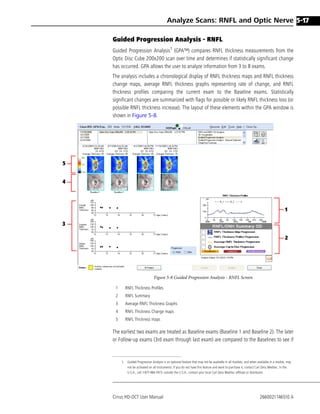
  • 1. Analyze Scans: RNFL and Optic Nerve 5-17 Guided Progression Analysis - RNFL Guided Progression Analysis1 (GPA™) compares RNFL thickness measurements from the Optic Disc Cube 200x200 scan over time and determines if statistically significant change has occurred. GPA allows the user to analyze information from 3 to 8 exams. The analysis includes a chronological display of RNFL thickness maps and RNFL thickness change maps, average RNFL thickness graphs representing rate of change, and RNFL thickness profiles comparing the current exam to the Baseline exams. Statistically significant changes are summarized with flags for possible or likely RNFL thickness loss (or possible RNFL thickness increase). The layout of these elements within the GPA window is shown in Figure 5-8. 5 4 1 3 2 Figure 5-8 Guided Progression Analysis - RNFL Screen 1 RNFL Thickness Profiles 2 RNFL Summary 3 Average RNFL Thickness Graphs 4 RNFL Thickness Change maps 5 RNFL Thickness maps The earliest two exams are treated as Baseline exams (Baseline 1 and Baseline 2). The later or Follow-up exams (3rd exam through last exam) are compared to the Baselines to see if 1. Guided Progression Analysis is an optional feature that may not be available in all markets, and when available in a market, may not be activated on all instruments. If you do not have this feature and want to purchase it, contact Carl Zeiss Meditec. In the U.S.A., call 1-877-486-7473; outside the U.S.A., contact your local Carl Zeiss Meditec affiliate or distributor. Cirrus HD-OCT User Manual 2660021146510 A
  • 2. 5-18 Analyze Scans: RNFL and Optic Nerve they have changed. All scans, including the 2nd Baseline, are registered to the first Baseline in order to ensure accurate correspondence from the first scan to the last scan. The average RNFL thickness value is displayed for each exam above its corresponding thickness map. There is an indication above each displayed exam to describe the registration performed. Prior to comparing scans, Cirrus registers them to the first Baseline scan using one of two methods. First, it attempts to use method R2, which is based on the blood vessels identified in the en face images of both scans. Method R2 uses translation and rotation to align the follow up scan to the baseline scan. If there is motion in either the baseline or the follow-up scans, the R2 method may not be possible because the blood vessels will not line up well enough. In this case, the center of the optic disc from the follow-up scan translated to the center of the optic disc of the first scan prior to making comparisons for the purposes of identifying change. This method is called R1. It does not include rotation. If the R1 method is used, you may observe additional variability at the superpixel level. This may affect detection of change in the RNFL Map. Note: Cirrus does not evaluate “progression of glaucoma,” which can only be assessed through evaluating changes in several clinical factors, including optic nerve head appearance and visual fields. GPA only refers to change in the nerve fiber layer thickness assessed by statistical analysis of certain Cirrus parameters. Such change of RNFL thickness may or may not be related to clinically relevant changes. GPA is not meant to diagnose. Diagnosis is the responsibility of the practitioner, who should base diagnosis on many parameters, including those not assessed by Cirrus. Guided Progression Analysis - Optic Nerve Head Guided Progression Analysis also includes features to follow changes to the optic nerve head. This includes the following: • A graphical plot of the Average Cup-to-Disc Ratio as a function of patient age using the same layout as the graphical plots of RNFL average thickness measurements versus patient age. This graphical plot is available on a second page of the analysis screen. You may access this page by selecting the ONH toggle button. • The GPA summary box has been expanded to include a colored checkmark whenever Possible Loss, Likely Loss, or Possible Increase has been detected using the Average Cup-to-Disc Ratio. Note that ACDR increases as the thickness of RNFL decreases. Therefore, ‘Possible Loss’ of RNFL is indicated by an increase in ACDR, and thus ‘Possible Loss’ is checked when an there is an increase in ACDR observed (that exceeds the expected variability of ACDR). • The RNFL thickness maps that are displayed as a function of time include a mask to indicate the location of the cup and disc boundaries. This display is similar to what is seen on the ONH & RNFL OU Analysis. Cirrus HD-OCT User Manual 2660021146510 A
  • 3. Analyze Scans: RNFL and Optic Nerve 5-19 Figure 5-9 Guided Progression Analysis - ONH In addition, there is a second page of the GPA report (not shown on the screen) that includes a table of the exam date and time, serial number of the instrument the exam was acquired with, signal strength, RNFL average thickness, RNFL inferior thickness, RNFL superior thickness, rim area, average cup-to-disc ratio, vertical cup-to-disc ratio and cup volume. Each cell for these values is colored to indicate when statistically significant change from baseline has occurred at the 1% and 5% level. You can configure the print of the GPA report to include the RNFL or ONH page only instead of the default, which is to print both pages. To do this, select Tools > Options, and then select the tab associated with GPA printouts. GPA Scan Selection • GPA automatically selects the appropriate scans from the most recent 8 visits. The automatic selection algorithm looks for scans with the highest signal strength from each previous visit. Scans with signal strength of 5 or lower will not be loaded automatically, although you may load them using the manual tool if necessary. The software automatically establishes the first two qualifying exams as the Baselines. You may override the GPA selections by choosing Guided Progression Analysis–Manual Selection. The report indicates when manual selection has been used to select the Cirrus HD-OCT User Manual 2660021146510 A
  • 4. 5-20 Analyze Scans: RNFL and Optic Nerve exams for the GPA analysis. A list of eligible scans will be displayed so that you may choose alternative scans, as shown in Figure 5-10. Figure 5-10 GPA Manual Selection of Scans The first Baseline scan is indicated by the letter B. All the rest of the scans to be included in the analysis are indicated by green check marks ( ). Scans that are not selected for the current analysis do not have any mark next to the scan. You may change an unchecked scan to be included by clicking on the scan. The green check mark toggles with each click. Changing the Baseline Image The Baseline image will always be the oldest image in the GPA sequence. Any images older than the Baseline image will not be included in the GPA. 1. Select Guided Progression Analysis–Manual Selection. 2. Select the desired scan for the Baseline. 3. Click on Set as Baseline. The letter B will indicate the Baseline exam. The exam you selected will be the first Baseline and the next qualified exam will be the second Baseline. The second Baseline exam is not indicated by a letter B. It will only be indicated by a green check mark. GPA will recalculate all follow up exam comparisons based on the new Baseline. Note: Baselines can be from the same day, but should be separated by at least a day. However, if the Baselines are separated by too great of a time period, change may have occurred between Baselines, which would make it more difficult to detect loss. Cirrus HD-OCT User Manual 2660021146510 A
  • 5. Analyze Scans: RNFL and Optic Nerve 5-21 Including Scans 1. Select Guided Progression Analysis–Manual Selection. 2. Click on the scan to include. A green check mark will appear next to the scan. 3. Repeat for any additional scans to be included. You may not permanently exclude scans from Guided Progression Analysis. If you find a scan unacceptable for inclusion in GPA, you should either delete the scan or de-select it from within the Guided Progression Analysis - Manual Selection dialog box. When exam selection is complete, click on Next to exit the selection screen and continue to the GPA analysis. The GPA exam selections made during this process are set as the new default exams for the patient. Subsequent use of GPA using the automatic exam selection option will use these exams and will automatically select any new exams completed after the last manually selected exam. Should you have more than 8 eligible exam dates, the first Follow-up (exam 3) will be removed from the list and replaced with the most recent exam. Note: If you use GPA Manual Selection for a standalone Cirrus, the scans you select for inclusion are used by default the next time you run Cirrus GPA for the current scan. If you use GPA Manual selection for a Cirrus that is connected to the FORUM Archive, then in order to recreate a GPA report with manually selected scans, you must choose GPA Manual selection and select the appropriate scans. They will not be selected by default. The two Baselines are used in GPA in two ways: 1. The two Baseline exams are included in the linear regression that determines the rate of change, confidence limits on that rate, and statistical significance of the trend for the summary parameters (Average RNFL Thickness Graphs, page 5-24). For this part of the analysis, no distinction is made between the two baseline points and later points. 2. The two Baseline exams are used to determine if Possible or Likely change has occurred. Two baselines are required to allow confirmation of change over multiple visits (Using Confirmation to Improve Specificity, page 5-29). RNFL Thickness and Change Maps The top of the GPA screen (Figure 5-11) displays from 3 to 8 RNFL Thickness maps chronologically from left to right. These allow you to visualize the change in RNFL thickness over time. The maps are labeled with the date and time of acquisition, serial number of the instrument on which the data was acquired, the signal strength of the scan, and information on the method of registration and Average RNFL thickness. The system automatically registers the enface OCT fundus images from the selected exams to the first Baseline exam. You can see a good example of registration in Figure 5-11. The images of the second Baseline scan and the two Follow up visits have been rotated to align with the first Baseline scan. This gives precise registration of the red Calculation Circle. Below each thickness map is the OCT fundus image from that exam. For the Follow-up scans (3rd through last), regions where RNFL thickness has exceeded the test-retest Cirrus HD-OCT User Manual 2660021146510 A
  • 6. 5-22 Analyze Scans: RNFL and Optic Nerve variability are highlighted. These maps are referred to as the RNFL Thickness Change Maps, and the highlighted areas are areas of statistically significant change. RNFL Thickness Change Maps help you: 1. look for local thinning of the RNFL by comparing observed change to the test-retest variability, and 2. confirm the instances of apparent change by tracking the changes over multiple visits. When no regions are flagged, no change has exceeded the test-retest variability. When a region is flagged yellow, it has changed relative to the two Baselines, but an additional scan is required to confirm that the change is likely. This is called “Possible Loss.” When a region is flagged red, then it has changed relative to the two Baselines, and furthermore, the same region on the previous exam had also changed by more than the expected test-retest variability. This is called “Likely Loss.” A region that is flagged lavender indicates an increase in thickness relative to the two Baselines. This may occur due to statistical fluctuations or poor data quality. For “Likely Loss,” “Possible Loss,” or “Possible Increase,” to be reported, at least 20 adjacent superpixels must show significant change. Figure 5-11 Comparison of RNFL Loss Over Time In Figure 5-11, the first change map under Exam 3, which is the first Follow-up exam, is generated by comparing Exam 3 to the Baseline images. The areas of significant change when first detected are displayed in yellow for “Possible Loss.” The next change map is generated by comparing Exam 4 (the current exam) to the Baseline images, and significant change is found in some of the same areas as the previous exam. Since this significant change has been seen two consecutive times, the areas of change are displayed in red for “Likely Loss.” Cirrus HD-OCT User Manual 2660021146510 A
  • 7. Analyze Scans: RNFL and Optic Nerve 5-23 RNFL Thickness Profiles The RNFL Thickness Profiles (Figure 5-12) plots RNFL thickness values around the Cirrus RNFL Calculation Circle. All of the OCT fundus images are overlaid with the red circle that shows where the thickness profile measurements are evaluated. The location of the red circle on the first Baseline exam is determined by the automatic algorithm that finds the center of the optic disc. Because the remaining scans are registered to the first Baseline scan, the same center and circle are used for all other scans. There are three curves: two for the current Baseline exams shown in gray (labeled B1 and B2), and one for the most recent examination shown in blue (labeled C for current). The profile analysis identifies moderate focal thinning in the RNFL thickness by comparing observed change in the RNFL Thickness Profiles to test-retest variability, and then looking for instances where the apparent change is confirmed over multiple visits. For “Likely Loss,” “Possible Loss,” or “Possible Increase,” to be reported, at least 14 adjacent A-scans must show significant change. This value was chosen to allow the TSNIT profile to be sensitive to defects of 20-degrees or more. Areas between the Baseline pair and the current exam that report significant change are displayed with “Possible Loss” shown in yellow, “Likely Loss” shown in red, and “Possible Increase” shown in lavender. Figure 5-12 RNFL Thickness Profiles Cirrus HD-OCT User Manual 2660021146510 A
  • 8. 5-24 Analyze Scans: RNFL and Optic Nerve Average RNFL Thickness Graphs The Average RNFL Thickness Graphs (Figure 5-13) identify global thinning in the retinal nerve fiber layer by calculating a trend over time. The trend must be confirmed over multiple visits. Statistically significant loss, based on comparisons to test-retest variability, is also required. The Average RNFL Thickness Graphs are calculated by averaging large portions of the profile — this is why they detect only global loss. Each chart displays parameter data from 3 to 8 exams plotted in chronological order. The vertical axis represents RNFL thickness values ranging from 0–175 micrometers, and the horizontal axis represents patient age, spanning five years. Figure 5-13 Average RNFL Thickness and ONH Cup-to-Disc Ratio Graphs Four graphs are presented (Figure 5-13): 1. A graph of the overall average thickness trend that shows the overall average thickness from the Cirrus RNFL Calculation Circle for each exam. 2. A graph of Average Cup-to-Disc Ratio. Note that “Possible Loss” (orange color coding) and “Likely Loss” (red color coding) are associated with a positive slope or increase in the measurement. 3. A graph of the average thickness trend for the superior quadrant of the RNFL Calculation Circle for each exam. 4. A graph of the average thickness trend for the inferior quadrant of the RNFL Calculation Circle for each exam. The individual points are highlighted to indicate when the value plotted has changed from Baseline by an amount more than the test-retest variability. Possible loss occurs when the rate of loss is statistically significant for only a single visit and is indicated by a yellow symbol. Likely loss occurs when the rate of loss is statistically significant for two visits in a row and is indicated by a red symbol. Possible increase occurs when the rate of gain is statistically significant and is indicated by a lavender symbol. Possible increase should only occur due to random fluctuations or due to problems with scan quality. These plots are fit using linear regression in order to calculate the rate of loss. The linear regression line is plotted on each graph whenever there is both “Likely Loss” and a significant linear trend (p < 5%). Confidence bands for the regression line are also shown. They are determined based on comparing the variability in the data to the rate of change. The slope (rate of change) is displayed in micrometers/year with 95% confidence interval values. For example, with a slope of –3.9 ±1.1, there is 95% confidence based on Cirrus HD-OCT User Manual 2660021146510 A
  • 9. Analyze Scans: RNFL and Optic Nerve 5-25 statistical analysis that the slope is between –2.8 and –5.0 μm/year. This is shown graphically in the shaded gray area. The graphical plots will show a rate of change and 95% confidence limits around that rate of change whenever at least 4 exams that span at least 2 years are loaded. If there are fewer than 4 scans loaded, or if there is less than two years between the first baseline and the current scan, no rate of change analysis will be provided. Note: Linear regression fits the data to a linear model, assuming that the measurements are independent, normally distributed, and that variability does not depend on the size of the measurement. If the observed measurements do not change linearly, the rate of change may still provide information about how the patient has changed during the period of examination, but it should not be used to predict future change. Linear regression is a statistical analysis, and should not replace clinical evaluation of the patient’s status and progress. RNFL/ONH Summary The RNFL Summary displays a color-coded summary box that alerts you if significant change has been detected. GPA has three different indicators for detecting RNFL change and one indicator for detecting ONH change, each with a check box in the summary: • RNFL Thickness Map Progression (best for focal change) • RNFL Thickness Profiles Progression (best for broader focal change) • Average RNFL Thickness Progression (best for diffuse change) • Average Cup-to-Disc Progression Cirrus HD-OCT User Manual 2660021146510 A
  • 10. 5-26 Analyze Scans: RNFL and Optic Nerve The summary box reports progressive change as one of “Possible Loss” (yellow), “Likely Loss” (red), or “Possible Increase” (lavender). “Possible Loss” means progressive loss has been detected once. “Likely Loss” means it has been confirmed by consecutive follow-up examinations. Shown below are examples of summary box displays. The yellow check marks in the RNFL Thickness Map Progression and RNFL Thickness Profiles Progression summary boxes above show Possible Loss. The red check mark in the RNFL Thickness Map Progression summary boxes above shows Likely Loss. The lavender check mark in the RNFL Thickness Map Progression summary box above shows Possible Increase. Cirrus HD-OCT User Manual 2660021146510 A
  • 11. Analyze Scans: RNFL and Optic Nerve 5-27 How to Read the GPA Report 1. Verify data quality Verify the images. Discard or retake images with poor registration and/or poor signal strength (SS < 6) whenever possible, or interpret with caution. On the Report, SS = Signal Strength. Verify image registration. How similar are the Baselines? Examine the RNFL Thickness profiles, Average RNFL Thickness graphs, and RNFL thickness maps. If the Baselines are not consistent, GPA will be less able to flag RNFL loss. 2. Examine GPA printout Review the color-code RNFL/ONH Summary box. A yellow “Possible Loss” summary box indicates additional follow-up visits are recommended to confirm change. A red “Likely Loss” summary box indicates statistically significant change is detected in the measurements. A lavender “Possible Increase” summary box could indicate high measurement variability. 3. Apply GPA results in context of the patient GPA reports statistically significant change for one eye, which may or may not be clinically significant. Rate of loss, locations of the detected loss, age of the patient, stage of the disease, and other clinical factors should be evaluated for clinical decisions. To confirm that RNFL loss is clinically significant, correlate your results with other clinical tests such as perimetry and IOP. 4. Consider Resetting the Baseline Scans It is prudent to occasionally review the current Baseline scans and consider changing to a more recent Baseline pair if there has been a significant change in the course of the patient’s care. A stable period of RNFL thickness may follow a period of RNFL thinning due to a change in therapy. This leveling off would be a good time to update the Baseline images. This will allow GPA to flag change from this new point in time instead of having the summary flags continuously checked off due to thinning that occurred at an earlier, less stable time. Cirrus HD-OCT User Manual 2660021146510 A
  • 12. Analyze Scans: RNFL and Optic Nerve 5-28 Statistical Significance Guided Progression Analysis compares an observed change with its expected test-retest variability, as illustrated in Figure 5-14. Cutoff Point for Flagging Possible Increase (i.e., /2 = 97.5%) Cutoff Point for Flagging Possible or Likely Loss (i.e., /2 = 2.5%) Measured RNFL Change Change considered within normal test-retest variability (2.5% to 97.5%) Figure 5-14 Distribution of Test-Retest Variability Statistically Significant Change from Baseline Guided Progression Analysis compares an observed change with its population test-retest variability. The test-retest variability was determined by performing an in-house repeatability and reproducibility study (results reported at ARVO 2008 in a poster, "Inter-Visit and Inter-Instrument Variability for Cirrus HD-OCT Peripapillary Retinal Nerve Fiber Layer Thickness Measurements" – M.R. Horne, T. Callan, M. Durbin, T. Abunto; Poster 4624, ARVO 2008). The difference between a current exam and the Baseline is assumed to have a normal distribution with a standard deviation determined from clinical measurements on subjects over a short period of time. Only 5% of paired measurements are expected to have an absolute difference more than 1.96 times the standard deviation of differences observed in an in-house reproducibility study of normals, which is the test-retest variability. This is also equal to 2.77 times the reproducibility standard deviation observed. Figure 5-14 illustrates a normal distribution of differences, centered at a mean difference of zero. The yellow line shows the cutoff for declaring ‘Possible Loss’ or 'Likely Loss' and the lavender line shows the cutoff for declaring ‘Possible Increase’. For any individual comparison of a measurement to Baseline, only 2.5% of measurements are expected to show change to the left of the yellow line when real loss has not occurred, and only 2.5% of measurements are expected to show change to the right of the lavender line. Because thickness maps and profiles have multiple points available for testing, the observed rate of false positives would be higher than 5% if the cutoff is set based on the 95% confidence limit depicted in Figure 5-11. To achieve a reasonable false positive rate of Cirrus HD-OCT User Manual 2660021146510 A
  • 13. Analyze Scans: RNFL and Optic Nerve 5-29 no more than 5% for any given visit, the limits are set at 99% for the TSNIT profile and 99.5% for the change map. Using Confirmation to Improve Specificity In order to increase the specificity of the measurement over multiple visits, Cirrus also requires that statistically significant change from Baseline be observed for at least two pairs of measurements when only three measurements are available, and for at least three pairs of measurements when four or more measurements are available. In this case, Cirrus will report ‘Possible Loss’ for a parameter. For example, a superpixel on the change map will be colored yellow, or the RNFL Profile will show a yellow region between the Baseline and current scans, or the Average Thickness plot will show a yellow symbol for that visit. If, on the following visit, these same conditions are met for the same parameter, Cirrus will report ‘Likely Loss’, because now the change has been flagged for more than one visit. These confirmation strategies help improve the specificity, and reduce the effects of individual outlier measurements. Note: RNFL thickness is expected to decrease slowly as a function of normal aging. The RNFL data collected for the normative database (RNFL and ONH Normative Databases on page 5-10) showed a rate of loss for overall thickness of -0.2 micrometers per year, with a 95% confidence interval of -0.25 to 0.13 micrometers per year. For superior thickness, the rate was -0.25 micrometers per year (-0.35, -0.15), and for inferior thickness, it was -0.3 micrometers per year (-0.42, -0.21). This slow rate of change is consistent with observations of RNFL thickness loss measured on Stratus OCT. All of these results are based on cross-sectional data, and an individual patient’s normal aging rate may vary. Because the exact rate of change for any individual is unknown, Cirrus reports the 95% confidence limits on the slope. In the usual statistical understanding, a rate of change would be considered statistically significant if the range of rates covered by the 95% confidence limits exclude zero. It may be more useful to note that if the 95% confidence bands include a rate consistent with normal aging, the observed change may be due to normal aging process rather than glaucomatous loss. 1. 2. 3. 4. 5. 6. 7. R. Gurses-Ozden, M. Durbin, T. Callan, M. Horne, K. Soules, Cirrus Normative Database Study Group, "Distribution of Retinal Nerve Fiber Layer Thickness Using Cirrus™ HD-OCT Spectral Domain Technology" Poster 4632, ARVO 2008. Ramakrishnan R, Mittal S, Sonal A, et al. Retinal nerve fibre layer thickness measurements in normal Indian population by optical coherence tomography. Indian J Ophthalmol. 2006;54:11-15. Sony P, Sihota R, Tewari Hem K, et al. Quantification of the retinal nerve fibre layer thickness in normal Indian Eyes with optical coherence tomography. Indian J Ophthalmol. 2004;52:303-309. Hougaard JL, Ostenfeld C, Heijl A, et al. Modeling the normal retinal nerve fiber layer thickness as measured by Stratus optical coherence tomography. Graefes Arch Clin Exp Ophthalmol. 2006. Budenz DL, Anderson DR, Varma R, et al. Determinants of normal retinal nerve fiber layer thickness by Stratus OCT. Ophthalmology. 2007;114:1046-1052. Parikh RS, Parikh SR, Sekhar GC, et al. Normal age-related decay of retinal nerve fiber layer thickness. Ophthalmology. 2007;114:921-926. Ronald S. Harwerth "Age-Related Losses of Retinal Ganglion Cells and Axons," Investigative Ophthalmology & Visual Science, October 2008, Vol. 49, No. 10. Cirrus HD-OCT User Manual 2660021146510 A
  • 14. 5-30 Analyze Scans: RNFL and Optic Nerve Advanced Visualization Analysis The Advanced Visualization Analysis (Figure 5-15) is available to view any Optic Disc Cube 200x200 scan. This analysis screen functions the same as described in Advanced Visualization on page 4-19. A similar printout is available for this analysis. For horizontal scans, left of scan equals left of scan display and right of scan equals right of scan display. For vertical scans, bottom of scan equals left of scan display and top of scan equals right of scan display. Figure 5-15 Advanced Visualization Analysis Screen Cirrus HD-OCT User Manual 2660021146510 A
  • 15. Analyze Scans: RNFL and Optic Nerve 5-31 Printouts See Reports and Printing on page 4-37 for more information. Stock Print Stock printout examples for for RNFL and Optic Nerve scans include: • ONH and RNFL Thickness Analysis Stock Printout, page 5-32 • Patient Education Page, page 5-33 • RNFL Thickness Analysis Printout, page 5-34 • Guided Progression Analysis Printout - Page 1, page 5-35 • Guided Progression Analysis (GPA) Printout - Page 2, page 5-36 Cirrus HD-OCT User Manual 2660021146510 A
  • 16. 5-32 Analyze Scans: RNFL and Optic Nerve ONH and RNFL Thickness Analysis Stock Printout The stock printout for ONH and RNFL Thickness Analysis includes all the information on screen when you click Print. There is also a second page for this printout: the Patient Education Page, An example is shown in Figure 5-17. To change the print default from one page to two, see Setting Print Configuration Defaults on page 4-39. Figure 5-16 ONH and RNFL Thickness Analysis Printout Cirrus HD-OCT User Manual 2660021146510 A
  • 17. Analyze Scans: RNFL and Optic Nerve 5-33 Patient Education Page Page 2 of the ONH and RNFL Thickness Analysis Stock Printout, the Patient Education Page, is shown below. Figure 5-17 Patient Education Page Cirrus HD-OCT User Manual 2660021146510 A
  • 18. 5-34 Analyze Scans: RNFL and Optic Nerve RNFL Thickness Analysis Stock Printout The stock printout for RNFL Thickness Analysis includes all the information on screen when you click Print. Figure 5-18 RNFL Thickness Analysis Printout Cirrus HD-OCT User Manual 2660021146510 A
  • 19. Analyze Scans: RNFL and Optic Nerve 5-35 Guided Progression Analysis (GPA) Printout - Page 1 The stock printout for Guided Progression Analysis includes all the information on screen when you click Print. Figure 5-19 Guided Progression Analysis Printout - Page 1 Cirrus HD-OCT User Manual 2660021146510 A
  • 20. 5-36 Analyze Scans: RNFL and Optic Nerve Guided Progression Analysis (GPA) Printout - Page 2 1DPH DVH *3$ ([DPSOH %DVH/LQH XUUHQW ,' ([DP 'DWH '2% ([DP 7LPH 0DOH 6HULDO 1XPEHU $0 30 *HQGHU 'RFWRU 6LJQDO 6WUHQJWK 0DUNLUUXV *XLGHG 3URJUHVVLRQ $QDOVLV *3$Œ
  • 21. %DVHOLQH %DVHOLQH ([DP ([DP 2' ([DP ([DP 26 ([DP ([DP 51)/ DQG 21+ 6XPPDU 3DUDPHWHUV ([DP 'DWH7LPH $0 %DVHOLQH $0 30 XUUHQW 30 %DVHOLQH 6HULDO 5HJLVWUDWLRQ 1XPEHU 0HWKRG 66 $YJ ,QI 6XS 5LP $YHUDJH 9HUWLFDO XS 51)/ 4XDGUDQW 4XDGUDQW $UHD XSWR XSWR 9ROXPH 7KLFNQHVV 51)/ 51)/ PPð
  • 23. —P
  • 24. —P
  • 25. —P
  • 26. 5DWLR 5DWLR 5 5 5 5HJLVWUDWLRQ 0HWKRGV 5 5HJLVWUDWLRQ EDVHG RQ WUDQVODWLRQ DQG URWDWLRQ RI 27 IXQGXV 5 5HJLVWUDWLRQ EDVHG RQO RQ WUDQVODWLRQ RI GLVF FHQWHU /LNHO /RVV 3RVVLEOH /RVV 3RVVLEOH ,QFUHDVH RPSDUHG WR EDVHOLQH VWDWLVWLFDOO VLJQLILFDQW ORVV RI WLVVXH GHWHFWHG )RU $YHUDJH 51)/ 6XSHULRU 51)/ ,QIHULRU 51)/ 5LP $UHD WKH YDOXHV KDYH GHFUHDVHG )RU XSWR'LVF 5DWLRV DQG XS 9ROXPH YDOXHV KDYH LQFUHDVHG RPSDUHG WR EDVHOLQH VWDWLVWLFDOO VLJQLILFDQW LQFUHDVH GHWHFWHG )RU $YHUDJH 51)/ 6XSHULRU 51)/ ,QIHULRU 51)/ 5LP $UHD YDOXHV KDYH LQFUHDVHG )RU XSWR'LVF 5DWLRV DQG XS 9ROXPH YDOXHV KDYH GHFUHDVHG 'RFWRU V 6LJQDWXUH RPPHQWV $QDOVLV (GLWHG 30 0DUF 6: 9HU RSULJKW DUO =HLVV 0HGLWHF ,QF $OO 5LJKWV 5HVHUYHG 3DJH RI Figure 5-20 Guided Progression Analysis Printout - Page 2 Cirrus HD-OCT User Manual 2660021146510 A
  • 27. Analyze Scans: RNFL and Optic Nerve 5-37 Performance of Cirrus HD-OCT RNFL Analysis Repeatability and Reproducibility CZM performed an in-house study on normal subjects to determine the inter-visit and inter-instrument repeatability of Cirrus RNFL thickness measurements. The repeatability and reproducibility (including effects of multiple visits and multiple instruments), along with the coefficient of variability, are shown in Table 5-1 on page 5-38. Similar results were also found in an independent study, which reported a coefficient of variability of 1.5% in normal subjects and 1.6% in patient eyes1. Comparison to Stratus OCT A study2 of normal subjects and subjects with glaucoma (N = 130) found that although there were differences between Stratus and Cirrus, the Pearson correlation coefficient for the average RNFL thickness was 0.953, indicating good correlation. However, they also found a systematic difference between Cirrus and Stratus RNFL measurements. Cirrus measures thicker than Stratus at thinner RNFL values and measures thinner at thicker (more normal) RNFL values. Measurements from the two systems should not be used interchangeably. 1. Vizzeri, G, Weinreb, RN, Gonzalez-Garcia, AO, Bowd, C, Medeiros, F, Sample, PA, Zangwill, LM: Agreement between spectral-domain and time-domain OCT for measuring RNFL thickness, Br J Ophthalmol, March 2009. 2. Knight OJ, Chang RT, Feuer WJ, Budenz DL. “Comparison of retinal nerve fiber layer measurements using time domain and spectral domain optical coherent tomography.” Ophthalmology. 2009 Jul;116(7):1271-7. Cirrus HD-OCT User Manual 2660021146510 A
  • 28. Analyze Scans: RNFL and Optic Nerve 5-38 Table 5-1 Repeatability and Reproducibility of Cirrus RNFL measurements for seventeen sectors, including the overall average thickness, four quadrants (temporal, superior, nasal, and inferior), and twelve sectors, labeled by clock hour, with the 9 o'clock hour most temporal, measured on 32 normal subjects. Mean Thickness (μm) Repeatability SD (μm) Reproducibility SD (μm) Repeatability Limita (μm) Reproducibility Limitb (μm) Average 93.1 1.33 1.35 3.72 3.78 Temporal 64.6 2.03 2.05 5.68 5.74 Superior 118.8 3.42 3.45 9.58 9.66 Nasal 68.6 2.19 2.24 6.13 6.27 Inferior 123.6 3.01 3.14 8.43 8.79 Clock hour 1 113.6 4.84 5.05 13.55 14.14 Clock hour 2 84.3 4.7 4.74 13.16 13.27 Clock hour 3 56.4 2.43 2.56 6.80 7.17 Clock hour 4 63.0 3.25 3.37 9.10 9.44 Clock hour 5 102.5 4.35 4.37 12.18 12.24 Clock hour 6 133.5 4.93 5.21 13.80 14.59 Clock hour 7 134.7 5 5.01 14.00 14.03 Clock hour 8 66.1 3 3 8.40 8.40 Clock hour 9 53.0 1.71 1.78 4.79 4.98 Clock hour 10 76.3 3.53 3.53 9.88 9.88 Clock hour 11 125.2 4.75 4.77 13.30 13.36 Clock hour 12 121.6 6.43 6.51 18.00 18.23 a. Repeatability Limit is the upper 95% limit for the difference between repeated results. Per ISO 5725-1 and ISO 5725-6, Repeatability Limit = 2.8 x Repeatability SD. b. Reproducibility Limit is the upper 95% limit calculated for the difference between results repeated with different operators on different instruments. Each subject was imaged three times each during three visits on a single instrument (Phase 1) or twice during a single visit on five instruments (Phase 2). Per the ISO quoted in the main text, Reproducibility limit = 2.8 x Reproducibility SD. Cirrus HD-OCT User Manual 2660021146510 A
  • 29. Anterior Segment Scan Acquisition and Analysis 6-1 ESF=^åíÉêáçê=pÉÖãÉåí=pÅ~å=^Åèìáëáíáçå= ~åÇ=^å~äóëáë This chapter explains how to use the Anterior Segment Scan Acquisition and Analysis features. Topics covered in this chapter include: • Acquiring Anterior Segment Scans, page 6-1 • Anterior Segment Scan Analysis, page 6-10 • The High Definition Image Analysis, page 6-11 • Anterior Segment Imaging, page 6-11 The Cirrus™ HD-OCT is primarily used for imaging and measuring structures in the posterior eye. By changing the focus of the OCT beam, it can also be used to image and measure structures in the anterior segment such as the cornea. This chapter provides instructions and information about imaging and measuring the anterior segment with the Cirrus HD-OCT. Acquiring Anterior Segment Scans These instructions address two scan acquisition options, and subsequent analyses, for the Anterior Segment. The acquire options are: • Anterior Segment Cube 512x128 • Anterior Segment 5 Line Raster The HD-OCT imaging specifications for anterior segment scanning are the same as described in the Specifications chapter of the Cirrus HD-OCT User Manual, within the central 0.5 mm depth and central 2 mm width of the displayed tomograms. The best imaging performance occurs in the center of the imaging region. Upon choosing an anterior segment scan, • The LSO illumination of the retina is turned off (Model 4000). • The internal fixation target is centered. • The iris illumination is dimmed by default. This is to avoid causing pupillary constriction. • You will hear a click as the internal lens is brought into position. Some controls and displays used for posterior eye scanning are not present for anterior segment image acquisition. These are: • The Center control (Z-offset) for the OCT scan display is not present. The OCT display can be centered vertically in the live OCT window by using the Chinrest control buttons or the mouse scroll wheel. • Even though there is no fundus image, the Focus control buttons are still available for adjusting the focus of the fixation target. The scan pattern is now displayed over the iris image. The scan pattern cannot be moved, and the size of the scan is fixed. The 5-line raster scans can be rotated. Cirrus HD-OCT User Manual 2660021146510 A
  • 30. 6-2 Anterior Segment Scan Acquisition and Analysis Anterior Segment Cube 512x128 This scan mode generates a volume of data through a 4 millimeter square grid by acquiring a series of 128 horizontal scan lines each composed of 512 A-scans. It also acquires a pair of high definition scans through the center of the cube in the vertical and horizontal directions that are composed of 1024 A-scans each. The Anterior Segment Cube 512x128 has the same scan characteristics as the Macular Cube 512x128. This scan can be used for measuring the central corneal thickness and create a 3-D image of the data. Choosing this option produces the Anterior Segment 512x128 Cube Acquire screen, Figure 6-1. Alignment Bars Figure 6-1 Acquire Screen, Anterior Segment Cube 512x128 Cirrus HD-OCT User Manual 2660021146510 A
  • 31. Anterior Segment Scan Acquisition and Analysis 6-3 Anterior Segment 5 Line Raster This mode scans through 5 parallel lines of equal length. This scan can be used to view high resolution images of the anterior chamber angle and cornea. The line length is fixed at 3 mm, but the rotation and spacing are adjustable. Each line is composed of 4096 A-scans. By default, the lines are horizontal and separated by 250 μm (0.25 mm), so that the 5 lines together cover 1 mm width. See Figure 3. Choosing this option produces the Anterior Segment 5 Line Raster Acquire Screen, Figure 2. Alignment Bars Figure 6-2 Acquire Screen, Anterior Segment 5 Line Raster Cirrus HD-OCT User Manual 2660021146510 A
  • 32. 6-4 Anterior Segment Scan Acquisition and Analysis Menu selections on the Acquire Screen Under the iris viewport, select this button to bring up the Custom Scan Pattern menu shown on the left. This allows you to adjust the rotation and spacing of the 5 Line Raster scan. All adjustments apply to all 5 lines jointly. • For Rotation (default 0 degrees is horizontal), click the up arrow (for counterclockwise rotation) or down arrow (for clockwise rotation) or type in a value to adjust the angle in the ranges of 0 to 90 or 270 to 359 degrees. Values typed in from 91 to 269 are automatically changed to the corresponding value 180 degrees opposite. • For line Spacing, you can select among the following options, in millimeters: 0 (five lines in same location), 0.01, 0.025, 0.05, 0.075, 0.125, 0.2, 0.25. Options and Reset buttons Each area has an Options button , which opens additional controls to adjust the image settings for that viewport. These controls include brightness, contrast and/or illumination. An example appears at left, for the iris image. Each area also has a Reset button , to return the settings to their default or initial positions. Alignment for Scanning the Central Cornea These instructions are applicable to both Anterior Segment 512x128 Cube Scan and the Anterior Segment 5 Line Raster. 1. From the ID Patient screen, click Acquire. 2. Before the patient puts his or her chin on the chinrest, click to select the desired scan type for either eye. You might hear a click sound as the auxiliary lens is moved into position. You can have the patient look at the internal fixation, which will always be straight ahead, or the external fixation device. You may optionally adjust the focus of the internal fixation for the patient using the manual Focus adjustment. 3. Adjust the region of the iris visible in the iris viewport. Coarse adjustments are made by using the X-Y controls to move the chinrest, as needed, until the pupil is visible. Clicking on a chinrest control arrow moves the eye in the direction indicated by the arrow. See Figure 6-3. X-Y Controls Align Z Controls Focus Click pupil center to align Figure 6-3 Iris viewport Cirrus HD-OCT User Manual 2660021146510 A
  • 33. Anterior Segment Scan Acquisition and Analysis 6-5 4. Center the pupil in the iris viewport by clicking the center of the pupil. Clicking anywhere in the iris viewport centers the field of view of the camera over the click point. 5. Adjust the distance to the patient using the chinrest control until you see the cornea in the OCT scan display. The mouse scroll wheel may be used to make fine adjustments. The best OCT image is obtained when the cornea is placed between the gray bars alongside the scan display. See Figure 6-4. Figure 6-4 OCT Placement 6. Click the Enhance button to improve the quality of the OCT image. Note: The Optimize button does not position the scan when taking Anterior Segment scans. It only performs the Enhance function. Note: If the patient’s cornea is perfectly centered, a strong reflection from the anterior cornea can produce bright artifacts in the OCT scan display (Figure 6-5). Cirrus HD-OCT User Manual 2660021146510 A
  • 34. 6-6 Anterior Segment Scan Acquisition and Analysis The scan alignment should be slightly offset from the center by adjusting the chinrest to avoid the corneal reflection. Figure 6-5 Corneal Reflection 7. When satisfied with the scan adjustments you have made, click on the Capture button. Figure 5 shows the Review Screen of the acquired data. 8. Click Save to save the image and return to the Acquire screen. If you do not want to save the image, click Try Again. Note: The instrument focuses the OCT beam onto the anterior segment. The OCT beam scans in an arc to allow the curved cornea to better fit into the 2 mm scan depth. This will cause the cornea to appear flat in the display during alignment and acquisition. This effect is partially corrected for after acquisition, so the cornea will appear with the expected curvature during review and analysis. Alignment for Scanning the Anterior Chamber Angle The Anterior Segment 5 line raster scan is the preferred scan type for imaging the anterior chamber angle because it can be rotated to image a cross section perpendicular to the limbus at any location. The following instructions apply when using any of the scans for anterior chamber angle imaging: 1. When scanning the anterior chamber, you will need to use the external fixation target to direct your patient’s gaze beyond the ocular lens housing. This moves the eye position to expose the limbus optimally, allowing scanning to be done without interference from the eyelids. In scanning the superior angle, the iris illumination light can be used as a fixation target. When imaging the temporal angle, it is helpful to cover the fellow eye, to allow the patient to fixate with the scanned eye. Cirrus HD-OCT User Manual 2660021146510 A
  • 35. Anterior Segment Scan Acquisition and Analysis 6-7 2. Adjust the area of the eye visible in the iris viewport until you are able to view the corneoscleral junction. Coarse adjustments are made by using the X-Y controls to move the chinrest, as needed, until the pupil is visible. Clicking on a chinrest control arrow moves the eye in the direction indicated by the arrow. The angle recess often appears shadowed by the sclera. Moving the scan slightly to another location along the limbus can sometimes avoid local shadowing. 3. Center the scan on the corneal limbus. The live OCT image should show the top of the cornea and should be almost horizontally aligned; a slight tilt is acceptable and can improve visualization of angle structures. Figure 6 shows a well-aligned scan and live OCT image. Note that the iris may not be well focused when scanning the angle. Figure 6-6 Anterior Chamber Angle Scan 4. Proceed with Enhance and Capture, then review the scan as described in the section on corneal scanning. Cirrus HD-OCT User Manual 2660021146510 A
  • 36. 6-10 Anterior Segment Scan Acquisition and Analysis Anterior Segment Scan Analysis To analyze or print either an Anterior Segment 5 Line Raster or an Anterior Segment Cube 512x128 scan, click Analyze from the ID Patient screen. Select the desired Anterior Segment scan from the scan list on the left then click on the appropriate analysis in the right-hand column. The Anterior Segment Analysis is the only analysis protocol available for the Anterior Segment Cube 512x128 scan. Figure 6-9 Anterior Segment Cube Analysis Screen The Anterior Segment Analysis screen (Figure 6-9) for the Anterior Segment Cube 512x128 scan displays the Iris Viewport with the scan area and scan navigators superimposed. The X slice (fast - B scan) is shown in the upper OCT image and the Y slice (slow - B scan) is shown below it. You may click on either OCT window and use the scroll wheel on the mouse to scroll through the slices or move the slice navigators in the Iris Viewport. Cirrus HD-OCT User Manual 2660021146510 A
  • 37. 6-12 Anterior Segment Scan Acquisition and Analysis The Central Cornea The corneal epithelium, Bowman's membrane and stroma are generally visible in the tomograms. (Figure 6-11). Measurement of the Central Corneal Thickness (CCT) can be done and is described in this manual. Epithelium Bowman’s Membrane Stroma Figure 6-11 Corneal Image Cirrus HD-OCT User Manual 2660021146510 A
  • 38. Anterior Segment Scan Acquisition and Analysis 6-13 The Anterior Chamber Angle The termination of the Descemet's membrane called Schwalbe's line, Schlemm's canal and anterior iris can often be seen and identified by trained clinicians. (Figure 6-12) The angle recess and scleral spur may be difficult to visualize at times. The shorter wavelength (840 nm) used by the Cirrus is more strongly scattered by the sclera and iris. Scattering by the sclera causes the angle recess to be often obscured in shadow. Schlemm’s canal Schwalbe’s line Iris Scleral spur Figure 6-12 Angle Scan Central Corneal Thickness (CCT) Measurement The operator is advised to evaluate the scanned image prior to making CCT measurements. The corneal image should have well-defined posterior and anterior surfaces, should not have excessive motion artifacts and corneal reflections on the central cornea, especially within the area where the measurement caliper is to be placed. The following conditions may affect the ability to obtain a good corneal image for CCT measurements: 1. Inability of the patient to maintain fixation, including patients with poor visual acuity. 2. Excessive corneal reflection resulting from certain intraocular lenses, corneal abrasions and corneal opacities. 3. Presence of contact lenses. The junction of some contact lenses and the corneal surface may not be easy to visualize. Patients should remove contact lenses prior to scanning for a CCT measurement. Cirrus HD-OCT User Manual 2660021146510 A
  • 39. 6-14 Anterior Segment Scan Acquisition and Analysis Central corneal measurements should be made at the apex of the cornea. To determine the apical area: 1. Estimate where the center of the pupil is on the image and move the scan navigators so that they intersect at that point. 2. Click on the ruler button, and align the ruler vertically against the mauve slice navigator on the horizontal scan. 3. The center of the cornea can be identified by moving the scan navigators throughout the entire scan volume and noting how the scans appear to move up and down within the box. The apical area, being closest to the instrument lens, will have the highest scans. By using the ruler as a reference point while moving the slice navigators, find the highest horizontal and vertical scans. 4. The CCT measurement should be made at the intersection of the highest horizontal and vertical scans, using the ruler on the horizontal scan. The intersection of the scans is identified by the position of the mauve slice navigator. Adjust the position of the ruler and place the white horizontal lines of the ruler ends on the anterior and posterior surfaces of the cornea. The measurement is in micrometers. See Figure 6-13 for the correct position of the ruler and the proper placement of the calipers. Figure 6-13 Positioning the Ruler Note: Vertical distances on the tomogram reliably show tissue thickness and tissue refractive index. Horizontal distances cannot be measured quantitatively on these tomograms. When applied to Anterior Segment Scans, the Ruler measures only vertical distances, with the scale factor set appropriately for measurements within the cornea. Note: The Ruler is calibrated for measuring corneal tissue only, based on the refractive index of the cornea. It is not calibrated for other tissue types. Note: The Anterior Scan Cube 512x128 will initially be presented in the High-definition mode. Click on the Show/Hide High-Resolution Images button to allow scrolling through the cube images or move a slice navigator to a different slice. Cirrus HD-OCT User Manual 2660021146510 A
  • 40. Anterior Segment Scan Acquisition and Analysis 6-15 Note: For the Anterior Segment 5 Line Raster scan, only the ruler buttons are available. Anterior Segment Function Buttons Many of the function buttons found on the Advanced Visualization screen for macula scans are found on the Anterior Segment Analysis screen for the Anterior Segment Cube 512x128 scan. You may toggle back and forth between the high-resolution images or add one or more rulers to the image to create measurements. Measurement ruler Delete all selected measurement lines Snap scan navigator lines to center Show/hide high resolution images Printing out any Anterior Segment analysis is done in the same way as Macular scans (see User Manual, Chapter 4, Reports and Printing). Typical printout styles appear below. Cirrus HD-OCT User Manual 2660021146510 A
  • 41. 6-16 Anterior Segment Scan Acquisition and Analysis Anterior Segment Cube 512x128 Printout The standard printout for the Anterior Segment Cube 512x128 analysis includes all the information on screen (Figure 6-14) when you click Print: Figure 6-14 Anterior Segment Analysis Printout, Anterior Segment Cube 512x128 Cirrus HD-OCT User Manual 2660021146510 A
  • 42. Anterior Segment Scan Acquisition and Analysis 6-17 Anterior Segment 5 Line Raster Printout The standard printout for the Anterior Segment 5 Line Raster analysis includes all the information on screen (Figure 6-15) when you click Print: Figure 6-15 High Definition Images Printout, Anterior Segment 5 Line Raster Cirrus HD-OCT User Manual 2660021146510 A
  • 43. 6-18 Anterior Segment Scan Acquisition and Analysis Cirrus HD-OCT User Manual 2660021146510 A
  • 44. Analyze Scans: 3D Visualization 7-1 ETF=^å~äóòÉ=pÅ~åëW=Pa=sáëì~äáò~íáçå You can perform a 3D Visualization analysis on any Cube exam. 1. Click the Analyze button to access the ANALYSIS screen. 2. From the list of patient exams, select any Cube exam. 3. Select 3D Visualization from the list of available analyses. The following 3D VISUALIZATION screen appears. Figure 7-1 3D Visualization Screen The image above depicts the default view. The cube boundaries are shown with white lines. Labels indicate the Nasal (N), Superior (S), Temporal (T), and Inferior (I) sides of the cube. The red, green, and blue spheres can be dragged along the matching colored lines to define slice planes. The default setting for the mouse is to rotate the image. You can zoom in or out using the mouse scroll button. The 3D Menu appears on the left side of the screen. An enlarged image of the menu is shown at left. The following functions are available in the menu. 3D Menu Cirrus HD-OCT User Manual 2660021146510 A
  • 45. 7-2 Analyze Scans: 3D Visualization View Settings Clicking on the View Settings button displays the dialog shown at left. The View Settings dialog allows you to make the following adjustments and options: • Sliders for Brightness, Contrast, Threshold, and Opacity (%) to adjust the tissue image appearance. The settings you apply are a matter of preference, though the default settings may serve as a useful starting point for both color and black and white images. Click Apply Defaults to return all display parameters to default settings. The Threshold slider allows the user to remove darker tissue in the image. For example, setting the threshold to 50 displays only the tissue that has an intensity value of more than 50. This enables the user to filter out parts of the image that are not of interest. • Use Same Transparency for all Pixels: The default setting is unchecked. This setting uses high transparency for darker pixels and low transparency for brighter pixels. These settings enables the user to see through darker tissue. The slider reduces or increases the transparency for all pixels by the same percentage. For example: setting the slider at 50% sets all pixels to 50% of their original value. When Use Same Transparency for all Pixels is checked, all pixels will share the same transparency value regardless of grayscale value. At slider position 0%, all pixels are completely opaque. At slider position 100%, all pixels are completely transparent. • Apply Intensity Filter: Check this box to view a specific tissue intensity and range. When this box is checked and Grayscale Intensity Range is set to 20, only tissues with intensity values from 80 to 120 are displayed. • Lighting: Check this box to change the lighting of the image. By default, the light source for the volume data is internal. Each pixel emits its own light like a light bulb. When the Lighting box is checked, the external light source can be changed so each pixel emits less light and more light comes from an outside light source. This action yields a more solid appearance. The External Light slider increased the external light source and decreases the internal light of the volume. At any time you can select one of the buttons at the bottom of the dialog: • Save As Global: Saves your changes and remembers them for all subsequent exams. It does not save the exam, just the settings. • Recall Global: Restores previously saved Global settings. • Apply Defaults: Restores the Default settings. Note: The Save As Global function in this dialog does not save the exam. You must use the Save Exam icon at the top of the screen to save the settings for the exam. Cirrus HD-OCT User Manual 2660021146510 A
  • 46. Analyze Scans: 3D Visualization 7-3 Show Settings Click on Show... in the Menu to display the Show Settings dialog below. Figure 7-2 ShowSettings Dialog Use the check boxes to show and hide surfaces and the volumes between or below surfaces. You can show or hide the cube boundary lines, and show or hide the view from the top or bottom of the box. The default settings are shown in the figure above. Clip Selector The Clip Selector allows you to select the whole cube or one of the four niches of the cube. Once you select a niche, move the colored spheres to cut into the corner to the desired depth. See the figure below for an example of a niche cut. Figure 7-3 Niche Cut Cirrus HD-OCT User Manual 2660021146510 A
  • 47. 7-8 Analyze Scans: 3D Visualization Straighten Volume Data reset buttons Figure 7-7 Volume Straighten Dialog This function allows you to adjust the surface of the scan to be horizontal in those cases where the retina is highly tilted. Click on Auto Straighten to automatically correct the image. The slider controls, number field, and up/down arrows are used to manually correct the image by adjusting the X and Z axes. Click on Reset to Zero to undo your corrections. The reset buttons (see figure above) located above each field allow you to reset X and Z axes separately. See the before and after figures below for an example. The left figure shows a tilted image, and the right figure shows the straightened image. Figure 7-8 Volume Straighten, Before (left) and After (right) Cirrus HD-OCT User Manual 2660021146510 A
  • 48. Analyze Scans: 3D Visualization 7-9 Transparent Surfaces Checking the Transparent Surfaces box allows you to view ILM, RNFL, or RPE as transparent surfaces. Use the sliders to adjust the transparency level. Note: When you use Transparent Surfaces, the image will have lower resolution. Reset Click Reset to return the image to its default settings. Print a Report Click on the Print icon to print a report. An example is shown below. Figure 7-9 Sample 3D Visualization Report Click on Save Exam to save the 3D View Settings for this exam. Cirrus HD-OCT User Manual 2660021146510 A