SlideShare ist ein Scribd-Unternehmen logo
1 von 18
Downloaden Sie, um offline zu lesen
Research Inventy: International Journal Of Engineering And Science
Vol.3, Issue 5 (July 2013), PP 01-18
Issn(e): 2278-4721, Issn(p):2319-6483, Www.Researchinventy.Com
1
Network Based Signal Recovery in Wireless Networks.
1
Mr. Mustak Pasha, 2
Prof. Asma Parveen
1
(Computer Science and Engineering, KBNCE/VTU Belgaum, India)
ABSTRACT : One of the severe problems in wireless interaction is the interference. Interference is caused
due to collision. In wireless network, the signal sent by a node will reach all its neighboring nodes. The signal
will collide, if a neighbor apart from the target node is receiving data from more than one node at the same
moment then the required signal will get cracked, which result in communication crash. In conventional
wireless networks, this crash of signals may cause communication failure if no division procedure is accepted.
This will corrupt the system performance, which include packet loss rate and energy effectiveness. In traditional
transmission when a terminal is receiving messages, its neighbors cannot transmit until receiving is finished,
such a mechanism is not efficient and a lot of bandwidth is wasted. The inefficiency of traditional wireless
transmission is mainly due to regulating the signal collision. In dispersed network such as ad hoc and some
sensor networks, the organize hub will not present in the network. This will increase the clash and interference.
In wireless networks, when signal crash, electromagnetic waves will overlap on each other. This strategy is
much more practical and easier to realize. Neither strict synchronization nor power control is needed among
the different terminals
KEYWORDS -Block fading, network coding, scheduling, time variant and wireless network.
I. INTRODUCTION
The BROADCAST nature of wireless medium is one of the principal features of wireless networks.
Although this feature may somewhat facilitate the broadcast communication, it usually causes interference and
collision in other scenarios. In a wireless network, signals sent by a terminal can reach all its neighbors, whereas
a terminal may simultaneously receive the signals from all its nearby nodes. In traditional wireless networks,
this collision of signals may cause transmission failure if no division technique is adopted. This will degrade the
system performance, such as the packet loss rate and energy efficiency. Moreover, in distributed networks such
as ad hoc and some sensor networks, the absence of control center will increase the opportunity of collision and
interference, which further reduces the transmission rate and brings about the inevitable hidden- and exposed-
node problems. Previous solutions to this problem mainly focused on how to avoid signal collision through
some well-developed protocols on the medium access control or network layer.
For example, shown in Fig. 1, the hidden node problem occurs in a point to multi-point network and is
defined as being one in which three (or more nodes) are present. Node A, Node B and Node C. It is possible that
in this case Node B can hear Node A (and vice versa) and Node B can hear Node C (and vice versa) BUT Node
C cannot hear Node A. In a CSMA/CA environment Nodes A and C would both properly transmit (they cannot
hear each other on the 'listen' phase so could both simultaneously and properly transmit a packet) but Node B
would get corrupted data. Nodes A and C are said to be 'hidden' from each other.
Fig. 1. The hidden nodes problem
Network Based Signal Recovery in Wireless …
2
The hidden nodes problem in wireless multi-hop sensor networks was mainly addressed with two
techniques: RTS/CTS and Carrier Sense Tuning .RTS/CTS was basically designed to reduce the number of
collisions due to hidden nodes by reserving the channel around both the sender and the receiver to protect frame
transmission from being corrupted by hidden nodes. However, this method presents several problems when used
in wireless multi-hop sensor networks:
• The energy consumption related to a RTS/CTS exchange is significant, data frames are usually small, the
collision probability is the same for data frames as for RTS/CTS, so it does not make any difference if the
technique is used or not
• It does not avoid collisions in multi-hop networks
• It may lower the network capacity due to the exposed node problem,
• It cannot be used for broadcast frames.
Several MAC protocols have proposed to use Carrier Sense Tuning to cope with the hidden node
problem .The key idea comes from the observation that hidden nodes cause Collisions, because their radio
carrier sense range is not large enough to sense ongoing transmissions they may collide with. Hence, a node
should tune its radio carrier sense range to make sure that when it transmits, there is no another transmission.
Although this method allows a node to detect ongoing transmissions, it is not suitable for all situations. For
example, it assumes a homogeneous radio channel for all nodes, which is not always possible because of
obstacles, different antenna height, etc. Even if the channel is homogeneous, it is not possible to increase the
carrier sense range of radio transceivers indefinitely due to physical limitations.
1.1 Use of RTS and CTS
Hidden Nodes are solved by the use of a RTS (request to send)/CTS (clear to send) protocol prior to
packet transmission. In our three node network above Node A sends a small RTS packet which is heard by Node
B which send a small CTS packet which is heard by both Nodes A and Node C. Node C will not transmit in this
case.
1.2 Node Identification
Each node in a 802.11 network is identified by its MAC address (exactly the same as Ethernet a 6 byte
- 48 bit value). Receiving nodes recognize their MAC address. A node wishing to send data initiates the process
by sending a Request to Send frame (RTS). The destination node replies with a Clear To Send frame (CTS).
Any other node receiving the RTS or CTS frame should refrain from sending data for a given time (solving the
hidden node problem). The amount of time the node should wait before trying to get access to the medium is
included in both the RTS and the CTS frame. This protocol was designed under the assumption that all nodes
have the same transmission ranges. RTS/CTS are an additional method to implement virtual carrier sensing in
Carrier sense multiple access with collision avoidance (CSMA/CA). By default, 802.11 rely on physical carrier
sensing only which is known to suffer from the hidden node problem. RTS/CTS packet size threshold is 0–2347
octets. Typically, sending RTS/CTS frames does not occur unless the packet size exceeds this threshold. If the
packet size that the node wants to transmit is larger than the threshold, the RTS/CTS handshake gets triggered.
Otherwise, the data frame gets sent immediately. IEEE 802.11 RTS/CTS mechanism could help solve exposed
node problem as well, only if the nodes are synchronized and packet sizes and data rates are the same for both
the transmitting nodes. When a node hears an RTS from a neighbouring node, but not the corresponding CTS,
that node can deduce that it is an exposed node and is permitted to transmit to other neighbouring nodes. If the
Fig. 2. Use of RTS/CTS protocol prior to packet Transmission
Network Based Signal Recovery in Wireless …
3
nodes are not synchronized (or if the packet sizes are different or the data rates are different) the problem may
occur that the sender will not hear the CTS or the ACK during the transmission of data of the second sender.
In this paper, we shall put forward some efficient signal recovery algorithms without the request of
synchronization and power control among multiple data streams. Thus, the strategy is much more practical and
easier to realize. With our proposed algorithms, since certain types of signal collision are allowed, the
throughput and efficiency of wireless networks can greatly be increased. In different types of wireless channels,
the waveforms of the received signals are different, thus requiring different algorithms to recover the useful
signals. In this paper, we shall put forward several algorithms for three types of wireless channels.
For additive white Gaussian noise (AWGN) and block-fading channels, where the attenuation is
constant during the transmission of one frame, the recovering algorithms for BPSK and π/4-QPSK modulated
signals will be developed, respectively, without loss of generality. For the time-variant channel, we must know
the amplitude of the interference signal at each sampling time because the attenuation varies during the
transmission of one frame. Two algorithms on signal recovery will be proposed for large and small coherent
times, respectively. Simulation results will show that the bit error rate (BER) of the recovered signal using our
developed schemes is almost the same as the transmission without interference, which proves the effectiveness
of our strategy based on network coding. The rest of this paper is organized as follows: The network model and
the scheduling strategy based on physical-layer network coding are discussed in Section II. In Section III, we
will present the signal-recovery algorithms for AWGN and block-fading channels. In Section IV, two
algorithms of signal recovery for time-variant channels will be put forward. The performance of the proposed
strategy and some other practical issues are discussed in Section V. Section VI illustrates the simulation results,
which demonstrate the effectiveness of our approach. Finally, we conclude this paper in Section VII.
II. NETWORK MODEL AND THE SCHEDULING STRATEGY
Our model of wireless networks is shown in Fig. 3, where the source terminals S1 and S2 intend to
transmit two frames of messages x

= {x1, . . . , xL} and y

= {y1, . . . , yL} to the receivers R1 and R2, respectively.
L is called the “frame length” here. The link between each pair of adjacent terminals is assumed to be half-
duplex, which means that each terminal can both transmit and receive messages from its neighbors, but cannot
simultaneously do them. Since R1 and R2 are both inside the transmission region of S1, x

can be received by the
two receivers at the same time. If S1 and S2 simultaneously transmit, the signal of y

will collide with that of x

at R2, which may result in the transmission failure in traditional systems. However, if R2 knows the content of x

,
it can eliminate the interference of x

and recover y

from the mixed signal. Each multi hop transmission
session in wireless networks can well be described by this linear network model. In fact, the model shown in
Fig. 3 is a special case. There may be multiple interference signals at R2. It will be shown that, as long as the
receiver knows the information on all the interference signals, it can recover its desired signal through our
algorithms with a very large probability.
Fig. 3. Model of wireless networks with signal collision.
Network Based Signal Recovery in Wireless …
4
For convenience, we only consider the scenario with just one interference signal when we develop the
algorithms in the following sections. However, all these algorithms can easily be generalized to the multi-
interference case. As mentioned in the previous section, the scheme on signal recovery depends on the channel
property. In AWGN and block-fading channels, the attenuation is taken to be constant during the transmission
of one frame. Thus, one only needs to estimate the delay and amplitude of the frame of interference signal, and
then the interference signal can be “subtracted” from the mixed signal to recover the useful signal. The single-
side power spectral density of the additive white noise is assumed to be N0/2. For the block-fading channel, the
attenuation is assumed to be a Raleigh variable with a mean square value of 1, and different frames are assumed
to suffer different and independent attenuations. However, in a general fading channel, if the attenuation varies
during the transmission of one frame, we have to estimate the sampling value of each symbol in the frame of the
interference signal. To develop an effective signal-recovery algorithm for time-variant channels, an appropriate
channel model that can characterize different coherent times is needed. ARMA (p, q) process is a simple
stochastic process model with the aforementioned property. It has been shown that for each random process, one
can find an autoregressive moving average (ARMA) process such that its mean square error from the given
process is as small as possible if p and q are large enough. The generating equation of an ARMA (p, q) process
is
qnqnnpnpnn vvAuAuA    ...... 1111 (1)
where iA is the attenuation at the sampling time it , and i is a pure Gaussian random process with mean
 and variance  2
. Without loss of generality, we assume that  = 0. Thus, iA is also a Gaussian random
variable. Given pnn AA  ,...,1 and qnn   ,...,1 , the conditional normal distribution function of nA is
),...,,,...,|( 11 qnnpnnn AAzAp  


















   

2
1 1
2
2
1
exp
2
1
p
i
q
j
jniini
εε
εvAuz
σπσ
=  







2
2
2
1
exp
2
1
nAz
 
(2)
where     
p
i
q
j jninin vAuA
1 11  is the conditional expectation value of nA . Since a Raleigh random
variable is the sum of the squares of two Gaussian variables with mean 0 and the same variances, both the in-
phase and quadrature attenuations of a Raleigh fading channel can be modeled by the ARMA processes. The
coefficients  iu and  iv in (1) can be figured out through the channel estimation, and the values of p and q are
chosen according to the tradeoff between the accuracy and complexity. If q = 0 in (1), the ARMA process is
reduced to an autoregressive (AR) process
....12 npnpnn AuAuA   (3)
The AR process is Markovian, which means that each An is only related to the former p attenuation
values. Since the AR process is easier in form, we will only present the signal recovery algorithms for the
channel modeled by the AR process in the latter part of this paper. For the general ARMA process, the
algorithms and corresponding deductions are similar. Next, we will briefly discuss the scheduling strategy based
on the signal-recovery algorithms. First, each terminal stores the frames it has recently received. Then, we add
the identifier of the frame to be sent in the next time slot to the RTS message. Each frame has a unique
identifier, which can be defined by the source address and the index of the frame. Thus, the terminal that
receives the RTS messages from its neighbors can decide whether they can simultaneously transmit according to
the identifier. If among all the frames to be sent there is only one unstored frame, the terminal will broadcast a
CTS message; otherwise, the terminal will reply a non-CTS message with the identifiers of the frames that may
cause unsolvable interference. Take, for example, in contrast to the traditional scheduling strategy, A is allowed
Network Based Signal Recovery in Wireless …
5
to transmit b in time slot 3. Then, B will receive a mixed signal of a and b. Since B has received a before time
slot 3, B can recover the data of b from the mixed signal through our algorithms developed later. In the next
time slot, B can forward the recovered b to the next relay C. Node C will then receive the mixed signal of a and
b in time slot 4 and recover b using the same method as before. In time slot 5, node A will transmit another
frame of data, namely, c, and so on. It can be seen that if the data stream is incessant, it will take an average of
two time slots to transmit one frame. Compared to with the one third frames per time slot in traditional
scheduling, the throughput is significantly increased.
2.1 Network Block Codes
Consider for a moment a simple unicast scenario shown in Fig.4 assume that the source is connected to
the destination through h edge-disjoint paths each consisting of unit-capacity edges, and that any t of these edges
can introduce errors. Note that an error can propagate only through the path on which it is introduced. Therefore,
the receiver will observe at most t corrupted symbols, and the source can send information at rate k to the
receiver by the means of an (h, k, 2t + 1) channel block code that maps k information symbols to h coded
symbols, and can correct any t random errors. The coded symbols will be sent simultaneously on the h edges,
thus using the “space” as the resource to accommodate for the redundancy introduced by the code, rather than
time as in classical channel coding where coded symbols are sent sequentially and errors occur at different time
slots. Consider now a multicast scenario where a source is connected to multiple receivers through an arbitrary
network with the min-cut between the source and each receiver equal to h. Note that if different sets of h edge
disjoint paths between the source and different receivers do not overlap, network coding is not necessary, and
the problem reduces to that of Fig. 4 for each receiver separately, and thus to classical channel coding.
Otherwise, we want to design the network code to protect the source message for each receiver.
Fig. 4. Simple unicast scenario
Definition. A network code is t-error correcting if it enables each receiver to correctly receive source
information as long as the number of edges that introduce errors is smaller than t. Unlike classical channel
codes, network error correction codes use coding operations not only at the source, but also at intermediate
nodes of the network. Therefore, an error introduced at a single edge may propagate throughout the network.
For simplicity we will assume that both the source and the channel (network) alphabet are Fq. Therefore, Fig. 4
at the source node, k information symbols are encoded into h coded symbols, which are then simultaneously
transmitted to the destination. The source produces qk
messages. If the network code is such that each receiver
can correctly decode if errors are introduced in up to t edges, then, for each receiver, the set of qk
h-dimensional
vectors at any h-cut corresponding to the qk
different source messages will be an (h, k) classical code that can
correct at least t errors. Therefore, the appropriate channel coding bounds connecting parameters q, h, k, and t
hold.
2.2 Bit Error Rate (BER):
Bit error Rate, sometimes bit error ratio (BER) is the most fundamental measure of system
performance. That is, it is a measure of how well bits are transferred end-to-end. While this performance is
affected by factors such as signal-to-noise and distortion, ultimately it is the ability to receive information error-
free that defines the quality of the link Bit error ratio (BER) is the number of bits received in error, divided by
the total number of bits received. It is the percentage of bits that have errors relative to the total number of bits
received in a transmission, usually expressed as ten to a negative power. For example, a transmission might
have a BER of 10-5
, meaning that on average, 1 out of every of 100,000 bits transmitted exhibits an error. The
BER is an indication of how often a packet or other data unit has to be retransmitted because of an error. If the
BER is higher than typically expected for the system, it may indicate that a slower data rate would actually
Network Based Signal Recovery in Wireless …
6
improve overall transmission time for a given amount of transmitted data since the BER might be reduced,
lowering the number of packets that had to be resent. The formulae to calculate the BER are used here as
follows:
Case-I: In this case, AWGN is generated by using „randn‟ function and multiplied by noise power data
sequence is generated by using „randsrc‟ function. Received data is obtained by adding AWGN and data bit
generated earlier. „sign‟ function is used to demodulate and recover data in noisy condition. „abs‟ function is
used to find absolute value and complex magnitude.
Case-II: In this case, AWGN is generated by using „randn‟ function and multiplied by signal power data
sequence is generated by using „randsrc‟ function and multiplied by signal power. Received data is obtained by
adding AWGN and data bit generated earlier. „sign‟ function is used to demodulate and recover data in noisy
condition and then multiplied by signal power. „abs‟ function is used to find absolute value and complex
magnitude.
To calculate the Bit Error Rate (BER):
Err-symbol=abs(recover_data-TX_data)
Total_err=length(find(Err_sysnbol))
BER=Total_err/N
III. SIGNAL-RECOVERY ALGORITHM FOR AWGN AND BLOCK-FADING CHANNELS
Additive white Gaussian noise (AWGN) is a channel model in which the only impairment to
communication is a linear addition of wideband or white noise with a constant spectral density (expressed as
watts per hertz of bandwidth) and a Gaussian distribution of amplitude. The model does not account for fading,
frequency selectivity, interference, nonlinearity or dispersion. However, it produces simple and tractable
mathematical models which are useful for gaining insight into the underlying behavior of a system before these
other phenomena are considered.
3.1 Channel capacity
The AWGN channel is represented by a series of outputs Yi at discrete time event index i. Yi is the sum
of the input Xi and noise, Zi, where Zi is independent and identically distributed and drawn from a zero-mean
normal distribution with variance n(the noise). The Zi are further assumed to not be correlated with the Xi.
Zi ~ N(0,n)
Yi = Xi + Zi ~ N(Xi, n)
The capacity of the channel is infinite unless the noise n is nonzero, and the Xi is sufficiently
constrained. The most common constraint on the input is the so-called "power" constraint, requiring that for a
codeword (x1, x2, ……, xk) transmitted through the channel, we have:


k
i
i Px
n 1
21
where P represents the maximum channel power. Therefore, the channel capacity for the power-constrained
channel is given by:
);(max)(..)( 2
YXIC
PXEtsxf 

Where f(x) is the distribution of X. Expand I(X;Y), writing it in terms of the differential entropy:
I(X;Y) = h(Y) – h(Y|X) = h(Y) – h(X+Z|X) = h(Y) – h(Z|X)
But X and Z are independent, therefore:
I(X;Y) = h(Y) – h(Z)
Evaluating the differential entropy of a Gaussian gives:
Network Based Signal Recovery in Wireless …
7
)2log(
2
1
)( enZh 
Because X and Z are independent and their sum gives Y:
nPZEZEXEXEZXEYE  )()()(2)()()( 2222
From this bound, we infer from a property of the differential entropy that
))(2log(
2
1
)( nPeYh  
Therefore the channel capacity is given by the highest achievable bound on the mutual information:
)2log(
2
1
))(2log(
2
1
);( ennPeYXI  
Where I(X;Y) is maximized when:
),0(~ PNX
Thus the channel capacity C for the AWGN channel is given by:







n
P
C 1log
2
1
3.2 Channel capacity and sphere packing
Suppose that we are sending messages through the channel with index ranging from 1 to M, the
number of distinct possible messages. If we encode the M messages to bits, then we define the rate R as:
n
M
R
log

A rate is said to be achievable if there is a sequence of codes so that the maximum probability of error
tends to zero as n approaches infinity. The capacity C is the highest achievable rate. Consider a codeword of
length n sent through the AWGN channel with noise level N. When received, the codeword vector variance is
now N, and its mean is the codeword sent. The vector is very likely to be contained in a sphere of
radius  Nn around the codeword sent. If we decode by mapping every message received onto the
codeword at the center of this sphere, then an error occurs only when the received vector is outside of this
sphere, which is very unlikely.
Each codeword vector has an associated sphere of received codeword vectors which are decoded to it
and each such sphere must map uniquely onto a codeword. Because these spheres therefore must not intersect,
we are faced with the problem of sphere packing. How many distinct code words can we pack into our n-bit
codeword vector? The received vectors have a maximum energy of n(P+N) and therefore must occupy a sphere
of radius  NPn  . Each codeword sphere has radius nN . The volume of an n-dimensional sphere is
directly proportional to rn
, so the maximum number of uniquely decodable spheres that can be packed into our
sphere with transmission power P is:
  
 
 NP
n
n
n
nN
NPn /1log
2
2
2
2



By this argument, the rate R can be no more than  NP /1log
2
1
 .
In the following section, we shall develop the signal-recovery algorithm in AWGN and block-fading
channels. In the following discussion, we assume that each frame has L symbols and that the delay D of relative
to y

is an integer and uniformly distributed on [−L, L]. In the following two parts, we will present the algorithms
on recovering y

from the mixed signal yx

 for BPSK and π/4 for QPSK modulations, respectively. For other
types of linear modulation, the principle of the recovery algorithm is similar.
Network Based Signal Recovery in Wireless …
8
3.3. Signal Recovery for BPSK Modulation
For BPSK modulation, the signals of x

and y

can mathematically be written as Ax(t − D) cos(ωt + γ)
and By(t) cos(ωt), respectively, where x(t), y(t) {1,−1}, and  is the phase shift of the carrier of x

from that of
y

. A and B are the signal amplitudes of x

and y

, respectively. Thus, the mixed signal of x

and y

at node R2
can be represented by
After demodulation and filtering, the sampled signal value of each symbol is
where k is the sampling index, and nk is the additive Gaussian noise with variance σ2
n = N0/2. For simplicity, let
yk = xk = 0 for k  [−L + 1, 0)  [L, 2L). We also assume that the carrier phase of y

and the local oscillator are
ideally synchronized, and the impact of carrier-phase errors will be discussed later in Section V. Since the
terminal R2 has received x

before, it can regenerate the sampling signal xk for 0 ≤ k < L. Then, one can compute
the correlation between {sk} and the delayed signal {xk−d}, where d(−L,L) is an integer, to estimate A and D.
That is
where A’ = A cos γ. Through effective source coding and channel coding, xk and yk will take the value of {−1, 1}
with equal probability and are independent of each other. Thus, we are satisfied that
According to the law of large numbers, if the frame length L is sufficiently large, 



12
/
L
Lk kk Ldxy and




12
/
L
Lk kk Ldxn will converge to 0 with very high probabilities. Moreover
is valid with a probability close to 1. Therefore, if one computes  dxsR ,,

for each d (−L,L) and find out the
maximum value, a reasonable estimation of A and D can be obtained by
(8)
where Dˆ = arg max−L<d<L  dxsR ,,

. By subtracting the estimated signal of x

from s

, y

can be recovered by
(9)
Network Based Signal Recovery in Wireless …
9
Note that if there are h frames of interference signals denoted by h
xxx

,...,, 21
instead of only one x

, all the
interferences can be eliminated by repeating the aforementioned process for h times. Here is a simplified
description of this algorithm.
Algorithm 1: Signal-Recovery Algorithm for BPSK in AWGN and Block-Fading Channels.
3.4 Recovering Algorithm for π/4-QPSK Modulation
π/4-QPSK modulation is widely used in wireless communications. For π/4-QPSK modulation, the input
bit stream is partitioned by a serial-to-parallel converter into two parallel data streams mI,k and mQ,k, each with a
symbol rate equal to half that of the incoming bit rate. Thus, we assume that the frame length is 2L symbols for
convenience. Then, the signal of π/4-QPSK is given by
(10)
where kkk   1 , and  4/3,4/3,4/,4/  k is related to mI,k and mQ,k according to a certain
mapping rule. Hence, the mixed signal at node B is
where γ is the phase difference between the carriers of x

and y

. D is the delay of x

relative to y

, whereas B
and A are the attenuations. Suppose that the phase shift of the local carrier from the carrier of y

is α. Then, after
demodulation, the sampled in-phase and quadrature signals are
respectively. nI,k and nQ,k are the Gaussian noises with mean 0. Similarly to BPSK, the sampled signal values of
x

and y

are set to be 0 if k < 0 or k ≥ L. The principle of signal recovery is similar to that for BPSK, and we
make use of the correlation between s(t) and x

. First, node R2 maps x

to   1
0


L
Kxk according to the same rule at
the transmitter. Then, let
Network Based Signal Recovery in Wireless …
10
In (12a),   LnnB
L
Lk
L
Lk dxkkQdxk
L
Lk kIdxkyk /sincoscos
12 12
,
12
, 




  



 

  converges to 0 as
L with a probability of 1. Moreover
is valid with a probability of 1. Then, the estimated value of A cos(γ − α) is given by
Similarly, one can estimate A sin(γ − α) from (12b) by
In the preceding equations
Hence, the interference of x

can be eliminated from the mixed signal s(t) as follows:
Network Based Signal Recovery in Wireless …
11
Finally, one can decode ykIˆ , ykQˆ and recover the original data of y

through base band differential
detection. Since this technique only computes 1 ykyk  for each k and the constant phase error α has no effect
on the decoding result, phase synchronization is not required here. In the aforementioned two algorithms, the
searching range of d is set to be (−L, L). In fact, it is not necessary to check all the values between −L and L.
The start and end times of a frame can be found out through its head and tailing bits, respectively. Then, the
length of the frame can be figured out. Although accurate duration of the mixed signal is difficult to detect, one
can still get an approximate estimation. In addition, whether D >0 or D <0 can be decided by checking the
identifier in the frame head. Thus, the searching range of d can greatly be shortened. For example, if we have
detected D >0 and the duration of the mixed signal is quite probably between N − l/2 and N + l/2 symbols.
Thus, the start time of x

is just L symbols before the termination time of the mixed signal, so D is probably
between N − l/2 − L and N + l/2 − L. Therefore, one can only consider d [N − l/2 − L, N + l/2 − L], where l is
a predefined parameter. The larger l is, the larger the probability of D [N − l/2 − L, N + l/2 − L] is. This way,
the estimation of D will be more accurate, and the complexity can largely be reduced.
IV. SIGNAL-RECOVERY ALGORITHM FOR TIME-VARIANT CHANNELS
In time-variant channels, the attenuation is not constant during one frame; thus, we need to estimate the
signal amplitude of each symbol of x

. However, if the channel slowly varies, the signal amplitude can still be
estimated by calculating the correlation. An easy and reasonable way is to calculate the glide correlation
between x

and s

. Suppose that the coherent time of the channel is the duration of M symbols. The signal
amplitude Ai of xi can be worked out by calculating the local correlation value as
For 2/2/ MLiM  . Then, let MRA ii /ˆ  be the estimated signal amplitude of xi. Here is the
algorithm for BPSK. (For QPSK4/ and other types of modulations, the ideas are the same).
Algorithm 2: Glide Correlation Algorithm on Signal Recovery for BPSK in Time Variant Channels.
If the coherent time M is relatively small, Ai may not be accurately estimated through the correlation,
and considerable interference may be induced. To deal with this problem, we will propose another signal-
Network Based Signal Recovery in Wireless …
12
recovery algorithm based on maximum likelihood. Without loss of generality, we shall take BPSK as an
example. The received mixed signal of x

and y

can be represented by
(18)
where B’k and yk are the amplitude and phase gains of the channel from S2 to R2 at the sampling time k,
respectively. Similarly, Av’ and xk are the channel gains from S1 to R2. θyk and θxk are the binary phase shifts
related to the information bits in x

and y

, respectively. Since θyk and θxk only have two possible values,
namely, 0 and π, we have
(19)
In (19), the attenuations ykkB cos' and xkkA cos' are Gaussian random variables modeled by the AR
processes. For simplicity, let Bk = ykkB cos' and Ak = xkkA cos' . Since Ak, Bk, and nk are independent of each
other, the joint distribution of the three variables is
where kB and kA are the expectations defined as (2), whereas x and y correspond to the variance  in
(2). Note that maximizing the joint probability equates to minimizing the power part in (20). Hence, one only
needs to solve the following optimization problem M:
Let us normalize the variables in the objective function by setting
  ,/
~
xDkDkDk AAA     ,/
~
ykkk BBB  and nkk nn /~  . Then, yk
H can be regarded as the square of
the Euclidean distance from  kkDk nBA ~,
~
,
~
 to the origin. Let ;coscos' DkDxkkykkk ABss   thus, the
solution to the problem M is as follows:
After solving (21), one can compute 1kB and DkA 1 as in (2). Then, the amplitude of the signals of
x

and y

, as well as the Gaussian noise, can recursively be figured out. Note that in (22), θyk is an unknown
variable. Fortunately, θyk has only finite values. One can first calculate yk
H for θyk = 0 and π, respectively, and
then select θyk = arg min yk
H as the decoding result of yk.
Note that one needs to know the delay D before performing the recursive calculation. This can be
achieved by the correlation method mentioned in Section III. Another problem is how to calculate the initial
values of kAˆ and kBˆ for k ≤ p [p is the order of the AR process defined in (3)]. If D > 0, which means x

is
sent later than y

, then the foreside of y

is not disturbed by x

. Since only the destroyed part of y

needs signal
Network Based Signal Recovery in Wireless …
13
recovery, one can set the initial values ykkk sB cos/ˆ  for k ≤ p, whereas the initial values of kAˆ can be set to
be 0. For D <0, the strategy is similar. In conclusion, the algorithm can be summarized as follows.
Algorithm 3: Signal-Recovery Algorithm by Maximizing the Posterior Probability for BPSK in Time-Variant
Channels.
Considering the errors in the aforementioned estimation of the initial values of Ak and Bk, we will adopt
the following method to improve the recovery result: First, Algorithm 3 is performed. Then, the obtained  kBˆ
and  DkA 
ˆ are regarded as the initial values of the attenuations. Take D > p, for example, and let the initial
values xkkk sA cos/'  and 1
ˆ
 Lk BB for L ≤ k < L+ p. Then, we calculate the attenuation values in reverse
order from the sampling time min {L, L + D} to max {0, D} according to Algorithm 3. After that, we combine
the two results and choose the one maximizing the likelihood. This method can make full use of the information
in the signal and, thus, can enhance the performance of the algorithm with a relatively high complexity. Since
the channel model in (1) is a forward generating equation, the inverted generating function needs to be derived
for the reverse computation. Note that the function in (1) is essentially a conditional distribution of a Markovian
process, and the joint distribution of multiple Gaussian random variables is still a Gaussian distribution
characterized by the covariance matrix and the means of the variables. The inverted generating function can be
obtained by calculating the co-variances between the attenuations at different sampling times. For the AR
process, however, the problem can be simplified by the following proposition.
Proposition 4.1: Given an AR process with mean 0 as in (3), the inverted generating function is
where ζn is a purely random Gaussian process with mean 0 and variance 2
 .
Network Based Signal Recovery in Wireless …
14
V. PERFORMANCE ANALYSIS
5.1 Performance Analysis
In the following section, we will analyze the performance of the recovery algorithms in the previous
sections. Due to the complexity of time-variant channels, we will only derive the analytical results for AWGN
and block-fading channels. The performance in time-variant channels will be shown by simulation results in the
next section. We shall consider the BER performance and the effect of phase errors, as well as the inter symbol
interference (ISI).
5.2.1 BER Performances
First, we consider BPSK modulation. From the correlation algorithm of signal recovery in Section III-
A, it can be seen that the resulting error bits in the recovered frame y

are mainly due to two factors, namely,
the Gaussian noise and estimation errors of A and D. If Dˆ = D, then from (9)
Thus, the total noise  

  
1
./'
LD
Dj kDjjDjjDkk nLxnxByxn Note that


 
1
/
LD
Dj DjjDk Lxnx is a Gaussian random variable with mean 0 and variance ./2
Ln According to the
central limit theorem, 

 
1
/
LD
Dj DjjDk Lxyx can be approximated by a Gaussian variable with mean 0 and
variance   ./1/ 2
LLDL  Thus, the variance of kn' is smaller than .// 222
'
2
LBLnnn   Thus the
conditional BER satisfies.
If L is large enough and the signal-to-noise ratio (SNR) of the channel is relatively small, the noise
induced by the correlation operation has a little effect on the total SNR and the BER performance. Consider the
probability  DDP ˆ subsequently. Suppose d [D − l/2, D + l/2], then
Where ./)22( 2222
LBA nz   According to (25) and (26), given A, B, and ,2
n the upper bound of the
BER is
Network Based Signal Recovery in Wireless …
15
From (27), it can be seen that the larger L is, the better the BER performance is. If L is large enough,
the noise induced by calculating the correlation can be neglected. For the block-fading channel, where A and B
are random variables, the upper bound of the BER is given by
where pA(A) and pB(B) are the Rayleigh distribution functions of A and B, respectively. The BER analysis of π/4-
QPSK in AWGN and block-fading channels is similar to that of BPSK. It must also be noted that there may be
error bits in x

itself, and this will impact  DDP ˆ and increase the BER of y

. Hence, it is necessary to adopt
a reliable channel coding scheme to avoid the propagation of error bits.
5.2.2 Impact of the Synchronization Error
Since the baseband differential detection technique only detects the phase difference between the
previous and current samples, the constant phase shift α will not affect the demodulation result of π/4-QPSK.
However, for BPSK, the phase error of the local carrier will reduce the power of the received signal and result in
BER performance degradation. Assume that in (4), the phase difference between y

and the local carrier is y ,
and that between x

and the local carrier is x . After coherent demodulation, the sampled signal is
After eliminating x

from the mixed signal s

, the power loss of y

is cos2
y . Suppose that y is uniformly
distributed on [−π, π], then the average power loss is
However, if differential PSK is adopted, the BER degradation due to the phase error is less than 1 dB for large
SNRs.
5.2 Effects in time domain (time variant)
In serial data communications, the AWGN mathematical model is used to model the timing error caused by
random jitter (RJ). The graph to the right shows an example of timing errors associated with AWGN. The
variable Δt represents the uncertainty in the zero crossing. As the amplitude of the AWGN is increased, the
signal-to-noise ratio decreases. This results in increased uncertainty Δt. When affected by AWGN, The average
number of either positive going or negative going zero-crossings per second at the output of a narrow band pass
filter when the input is a sine wave is:
Network Based Signal Recovery in Wireless …
16
Where
 f0 = the center frequency of the filter
 B = the filter bandwidth
 SNR = the signal-to-noise power ratio in linear terms
5.2 Effects in phasor domain
In modern communication systems, band limited AWGN cannot be ignored. When modeling band
limited AWGN in the phasor domain, statistical analysis reveals that the amplitudes of the real and imaginary
contributions are independent variables which follow the Gaussian distribution model. When combined, the
resultant phasor's magnitude is a Rayleigh distributed random variable while the phase is uniformly distributed
from 0 to 2π.
The graph to the right shows an example of how band limited AWGN can affect a coherent carrier signal.
The instantaneous response of the Noise Vector cannot be precisely predicted; however its time-averaged
response can be statistically predicted. As shown in the graph, we confidently predict that the noise phasor will
reside inside the 1σ circle about 38% of the time; the noise phasor will reside inside the 2σ circle about 86% of
the time; and the noise phasor will reside inside the 3σ circle about 98% of the time.
VI. SIMULATION RESULTS
In this section, we will present the sample simulation results to further investigate the performance of
the proposed signal recovery algorithms. In the simulation, we adopt the network model shown in Fig. 3, where
y

is the desired information, and x

acts as the interference. The delay of x

relative to y

is uniformly
distributed in [−L, L]. In block-fading channels, the amplitudes of y

and x

are set to be independent Rayleigh
random variables with variance 1. In AWGN channels, the amplitude of y

is set to be constant 1 and that of x

is set to be a random variable uniformly distributed in [−1, 1]. Fig. 4 shows the matching probability  DDP ˆ
versus different frame lengths for both BPSK and π/4-QPSK modulations in the AWGN channel. In this figure,
we set d [−L, L]. It can be seen that  DDP ˆ increases as L becomes larger, which is consistent with the
theoretical analysis. For the frame length L = 5000,  DDP ˆ is more than 95% for BPSK and 90% for π/4-
QPSK. This matching probability is acceptable since most wireless frames are not very short. The mismatching
cases mainly result from the fact that the amplitude of x

is too small. In these cases, x

brings about little
interference to y

and, thus, can be treated as common noise. Note the matching probability for BPSK is larger
than that for π/4-QPSK, and this is mainly because for BPSK, ykxk−D has only two possible values, namely, 1
and −1. Whereas for π/4-QPSK, cos(θyk−θxk−d−α) and sin(θyk−θxk−d−α) have eight possible values, respectively.
Thus, the variance of R( s

, x

, d) (d  D) in (5) is much smaller than that in (12). Fig. 5 shows the probability
 DDP ˆ under different SNRs. It can be seen that the power of noise has little impact on
Fig. 9. Zero-Crossings of a Noisy Cosine
Network Based Signal Recovery in Wireless …
17
 DDP ˆ under large frame lengths and moderate SNRs. The uppermost curve is the result of the method
mentioned in the last paragraph in Section III with l = 3, and the match probability is much larger than that with
d [−L,L]. Figs. 6 and 7 illustrate the BER performance of the recovery algorithms under different SNRs for
AWGN and block-fading channels, respectively. For BPSK modulation, SNR = ,/ 22
nB  where B is the
amplitude of y

, and σ2n is the power of the additive white noise. For π/4-QPSK, we define SNR = ,/ 22
nB 
where n
2
 is the variance of both nI,k and nQ,k in (11). Note that this definition is different from the standard
definition of SNR for π/4-QPSK; thus, there is a constant shift from the curves of π/4-QPSK to that of BPSK. In
Fig. 6, the BER of the algorithm with small L is larger than that with big L under high SNRs. Moreover, the
transmission without interference and that with interference but adopting our recovery algorithm have almost
the same BER under low SNRs, even if L is as small as 100. Fig. 7 shows the similar result in Rayleigh block-
fading channels. Thus, the two figures indicate that the algorithm will bring about little additional noise to the
desired signal if L is not too small. Therefore, with a proper frame length, the transmission capacity can be
approached by our strategy.
Network Based Signal Recovery in Wireless …
18
Fig. 8 shows the BER performance of the two algorithms in Section IV in a time-variant channel. The star curve
is for the scenario with no interference. The BER curves with circles and triangles are obtained through
Algorithms 2 and 3, respectively. Here, we use an AR process An − 0.99An−1 = εn as the channel model. We set
 nAVar = 10, and thus, σε = 1.41. Again, the delay  LLD , . Comparing the value of σε with  nAVar ,
one can see that the attenuation of the channel varies rather rapidly. From our simulation, the attenuation value
changes from positive to negative within an average duration of about 20 symbols. From the simulation result it
is show that our algorithms are able to remove almost all the interference.
VII. CONCLUSION
In this paper, we have proposed a signal-recovery scheme based on the physical-layer network coding,
which can eliminate the interference signal and recover the useful information from the mixed signal. By this
scheme, a new scheduling strategy, which allows a certain kind of signal collision without division techniques,
can be realized, and the throughput in wireless networks can greatly be increased. We have developed the
signal-recovery algorithms for AWGN, block-fading, and time-variant channels, respectively. For AWGN and
block fading channels, we made use of the correlation between the known information and the received signals
at the relay nodes to separate the desired signal from the mixed signal. For time variant channels, if the coherent
time is large enough, a glide correlation operation can eliminate the interference signal. A key feature of the
proposed physical layer network coding strategy is that neither synchronization nor power control among the
different transmitters is needed, thus making it well suited for distributed networks. By making of Theoretical
analysis and simulation results have shown that the signal-recovery algorithms can largely eliminate the
interference from the mixed signal.
REFERENCES
[1] A. Bachir, D. Barthel, M. Heusse, and A. Duda, “Hidden nodes avoidance in wireless sensor networks,” in Proc. Int. Conf.
Wireless Netw., Commun. Mobile Comput., Jun. 13–16, 2005, pp. 612–617
[2] Kaveh Pahlavan, “Wireless information networks examines sensor and mobile ad-hoc networks”, International journal of
wireless information, ISSN: 1068-9605, 2010, J.No. 10776
[3] T. C. Keong, presented at the Ad hoc mobile wireless networks: Protocols Syst. Conf., 2002.
[4] S. A. Aly and A. E. Kamal. Network protection codes against link failures using network coding. In Proc. Of IEEE 2008 Global
Telecommunications Conference, Dec. 2008.
[5] Morgan Kaufmann, “Wireless Communications and Networking”, Jul 28, 2010
[6] Jochen H. Schiller. “Mobile Communications”, Addison-Wesley, 2003
[7] Theodore S. Rappaport, “Wireless Communications – Principles and Practice”, Dorling Kindersley, 2009
[8] IETF “Mobile ad-hoc Networks (manet), http://www.ietf.org/html.charters/manet-charter.html
[9] Wireless Networking and Mobile IP”, http://www.cse.wustl.edu/~jain/refs/wir_book.html
[10] Wireless Networking – online references”, “Mobile multimedia and communication”, http://www.mobile3q.com/,
http://www.wirelessadvisor.com.
[11] Rober Spalding, “Storage Networks: The Complete Reference”, ISBN: 0072224762, McGraw-Hill/Osborne © 2003.

Weitere ähnliche Inhalte

Was ist angesagt?

WT - Circuit & Packet switching
WT - Circuit & Packet switchingWT - Circuit & Packet switching
WT - Circuit & Packet switchingvinay arora
 
A THROUGHPUT ANALYSIS OF TCP IN ADHOC NETWORKS
A THROUGHPUT ANALYSIS OF TCP IN ADHOC NETWORKSA THROUGHPUT ANALYSIS OF TCP IN ADHOC NETWORKS
A THROUGHPUT ANALYSIS OF TCP IN ADHOC NETWORKScsandit
 
VTU 8TH SEM CSE ADHOC NETWORKS SOLVED PAPERS OF JUNE-2014 DEC-14 & JUNE-2015
VTU 8TH SEM CSE ADHOC NETWORKS SOLVED PAPERS OF JUNE-2014 DEC-14 & JUNE-2015VTU 8TH SEM CSE ADHOC NETWORKS SOLVED PAPERS OF JUNE-2014 DEC-14 & JUNE-2015
VTU 8TH SEM CSE ADHOC NETWORKS SOLVED PAPERS OF JUNE-2014 DEC-14 & JUNE-2015vtunotesbysree
 
Network Layer,Computer Networks
Network Layer,Computer NetworksNetwork Layer,Computer Networks
Network Layer,Computer Networksguesta81d4b
 
Dcn data link_layer
Dcn data link_layerDcn data link_layer
Dcn data link_layermangal das
 
Enhancement of Improved Balanced LEACH for Heterogeneous Wireless Sensor Netw...
Enhancement of Improved Balanced LEACH for Heterogeneous Wireless Sensor Netw...Enhancement of Improved Balanced LEACH for Heterogeneous Wireless Sensor Netw...
Enhancement of Improved Balanced LEACH for Heterogeneous Wireless Sensor Netw...acijjournal
 
11.signal strength based congestion control in manet
11.signal strength based congestion control in manet11.signal strength based congestion control in manet
11.signal strength based congestion control in manetAlexander Decker
 
4..[26 36]signal strength based congestion control in manet
4..[26 36]signal strength based congestion control in manet4..[26 36]signal strength based congestion control in manet
4..[26 36]signal strength based congestion control in manetAlexander Decker
 
Performance analysis of CSMA/CA and TDMA MAC protocols in Wireless Mesh Netw...
Performance analysis of CSMA/CA and TDMA  MAC protocols in Wireless Mesh Netw...Performance analysis of CSMA/CA and TDMA  MAC protocols in Wireless Mesh Netw...
Performance analysis of CSMA/CA and TDMA MAC protocols in Wireless Mesh Netw...Pranjal Das
 
Circuit and packet_switching
Circuit and packet_switchingCircuit and packet_switching
Circuit and packet_switchinghoanv
 
Wireless Sensor Networks LEACH & EDEEC
Wireless Sensor Networks LEACH & EDEECWireless Sensor Networks LEACH & EDEEC
Wireless Sensor Networks LEACH & EDEECYogesh Fulara
 
Circuit switching packet switching
Circuit switching  packet  switchingCircuit switching  packet  switching
Circuit switching packet switchingSneha Dalvi
 
Performance Evaluation of a Layered WSN Using AODV and MCF Protocols in NS-2
Performance Evaluation of a Layered WSN Using AODV and MCF Protocols in NS-2Performance Evaluation of a Layered WSN Using AODV and MCF Protocols in NS-2
Performance Evaluation of a Layered WSN Using AODV and MCF Protocols in NS-2csandit
 

Was ist angesagt? (19)

WT - Circuit & Packet switching
WT - Circuit & Packet switchingWT - Circuit & Packet switching
WT - Circuit & Packet switching
 
A THROUGHPUT ANALYSIS OF TCP IN ADHOC NETWORKS
A THROUGHPUT ANALYSIS OF TCP IN ADHOC NETWORKSA THROUGHPUT ANALYSIS OF TCP IN ADHOC NETWORKS
A THROUGHPUT ANALYSIS OF TCP IN ADHOC NETWORKS
 
Seamless and Secured wide Fidelity enhancement in moving vehicles Using Eeack...
Seamless and Secured wide Fidelity enhancement in moving vehicles Using Eeack...Seamless and Secured wide Fidelity enhancement in moving vehicles Using Eeack...
Seamless and Secured wide Fidelity enhancement in moving vehicles Using Eeack...
 
Packet switching
Packet switchingPacket switching
Packet switching
 
VTU 8TH SEM CSE ADHOC NETWORKS SOLVED PAPERS OF JUNE-2014 DEC-14 & JUNE-2015
VTU 8TH SEM CSE ADHOC NETWORKS SOLVED PAPERS OF JUNE-2014 DEC-14 & JUNE-2015VTU 8TH SEM CSE ADHOC NETWORKS SOLVED PAPERS OF JUNE-2014 DEC-14 & JUNE-2015
VTU 8TH SEM CSE ADHOC NETWORKS SOLVED PAPERS OF JUNE-2014 DEC-14 & JUNE-2015
 
Network Layer,Computer Networks
Network Layer,Computer NetworksNetwork Layer,Computer Networks
Network Layer,Computer Networks
 
Dcn data link_layer
Dcn data link_layerDcn data link_layer
Dcn data link_layer
 
Enhancement of Improved Balanced LEACH for Heterogeneous Wireless Sensor Netw...
Enhancement of Improved Balanced LEACH for Heterogeneous Wireless Sensor Netw...Enhancement of Improved Balanced LEACH for Heterogeneous Wireless Sensor Netw...
Enhancement of Improved Balanced LEACH for Heterogeneous Wireless Sensor Netw...
 
Leach protocol
Leach protocolLeach protocol
Leach protocol
 
11.signal strength based congestion control in manet
11.signal strength based congestion control in manet11.signal strength based congestion control in manet
11.signal strength based congestion control in manet
 
4..[26 36]signal strength based congestion control in manet
4..[26 36]signal strength based congestion control in manet4..[26 36]signal strength based congestion control in manet
4..[26 36]signal strength based congestion control in manet
 
8 Packet Switching
8 Packet Switching8 Packet Switching
8 Packet Switching
 
Performance analysis of CSMA/CA and TDMA MAC protocols in Wireless Mesh Netw...
Performance analysis of CSMA/CA and TDMA  MAC protocols in Wireless Mesh Netw...Performance analysis of CSMA/CA and TDMA  MAC protocols in Wireless Mesh Netw...
Performance analysis of CSMA/CA and TDMA MAC protocols in Wireless Mesh Netw...
 
Circuit and packet_switching
Circuit and packet_switchingCircuit and packet_switching
Circuit and packet_switching
 
Wireless Sensor Networks LEACH & EDEEC
Wireless Sensor Networks LEACH & EDEECWireless Sensor Networks LEACH & EDEEC
Wireless Sensor Networks LEACH & EDEEC
 
Circuit switching packet switching
Circuit switching  packet  switchingCircuit switching  packet  switching
Circuit switching packet switching
 
VLAN on packet Tracer
VLAN on packet TracerVLAN on packet Tracer
VLAN on packet Tracer
 
Performance Evaluation of a Layered WSN Using AODV and MCF Protocols in NS-2
Performance Evaluation of a Layered WSN Using AODV and MCF Protocols in NS-2Performance Evaluation of a Layered WSN Using AODV and MCF Protocols in NS-2
Performance Evaluation of a Layered WSN Using AODV and MCF Protocols in NS-2
 
Thesis-Final-slide
Thesis-Final-slideThesis-Final-slide
Thesis-Final-slide
 

Andere mochten auch

Research Inventy : International Journal of Engineering and Science
Research Inventy : International Journal of Engineering and ScienceResearch Inventy : International Journal of Engineering and Science
Research Inventy : International Journal of Engineering and Scienceinventy
 
Research Inventy : International Journal of Engineering and Science
Research Inventy : International Journal of Engineering and ScienceResearch Inventy : International Journal of Engineering and Science
Research Inventy : International Journal of Engineering and Scienceinventy
 
Research Inventy : International Journal of Engineering and Science
Research Inventy : International Journal of Engineering and ScienceResearch Inventy : International Journal of Engineering and Science
Research Inventy : International Journal of Engineering and Scienceinventy
 
D042021027
D042021027D042021027
D042021027inventy
 
A03120105
A03120105A03120105
A03120105inventy
 
B04102026
B04102026B04102026
B04102026inventy
 
Research Inventy : International Journal of Engineering and Science
Research Inventy : International Journal of Engineering and ScienceResearch Inventy : International Journal of Engineering and Science
Research Inventy : International Journal of Engineering and Scienceinventy
 
B044010019
B044010019B044010019
B044010019inventy
 
A0320107
A0320107A0320107
A0320107inventy
 
A043001006
A043001006A043001006
A043001006inventy
 
Research Inventy : International Journal of Engineering and Science
Research Inventy : International Journal of Engineering and ScienceResearch Inventy : International Journal of Engineering and Science
Research Inventy : International Journal of Engineering and Scienceinventy
 
Research Inventy : International Journal of Engineering and Science
Research Inventy : International Journal of Engineering and ScienceResearch Inventy : International Journal of Engineering and Science
Research Inventy : International Journal of Engineering and Scienceinventy
 
B04206015
B04206015B04206015
B04206015inventy
 
Research Inventy : International Journal of Engineering and Science
Research Inventy : International Journal of Engineering and ScienceResearch Inventy : International Journal of Engineering and Science
Research Inventy : International Journal of Engineering and Scienceinventy
 
Analysis of Near-Far Problem using Power Control Technique for GNSS based App...
Analysis of Near-Far Problem using Power Control Technique for GNSS based App...Analysis of Near-Far Problem using Power Control Technique for GNSS based App...
Analysis of Near-Far Problem using Power Control Technique for GNSS based App...inventy
 
C032017020
C032017020C032017020
C032017020inventy
 
Research Inventy : International Journal of Engineering and Science
Research Inventy : International Journal of Engineering and ScienceResearch Inventy : International Journal of Engineering and Science
Research Inventy : International Journal of Engineering and Scienceinventy
 
C0312010014
C0312010014C0312010014
C0312010014inventy
 
H042036039
H042036039H042036039
H042036039inventy
 

Andere mochten auch (19)

Research Inventy : International Journal of Engineering and Science
Research Inventy : International Journal of Engineering and ScienceResearch Inventy : International Journal of Engineering and Science
Research Inventy : International Journal of Engineering and Science
 
Research Inventy : International Journal of Engineering and Science
Research Inventy : International Journal of Engineering and ScienceResearch Inventy : International Journal of Engineering and Science
Research Inventy : International Journal of Engineering and Science
 
Research Inventy : International Journal of Engineering and Science
Research Inventy : International Journal of Engineering and ScienceResearch Inventy : International Journal of Engineering and Science
Research Inventy : International Journal of Engineering and Science
 
D042021027
D042021027D042021027
D042021027
 
A03120105
A03120105A03120105
A03120105
 
B04102026
B04102026B04102026
B04102026
 
Research Inventy : International Journal of Engineering and Science
Research Inventy : International Journal of Engineering and ScienceResearch Inventy : International Journal of Engineering and Science
Research Inventy : International Journal of Engineering and Science
 
B044010019
B044010019B044010019
B044010019
 
A0320107
A0320107A0320107
A0320107
 
A043001006
A043001006A043001006
A043001006
 
Research Inventy : International Journal of Engineering and Science
Research Inventy : International Journal of Engineering and ScienceResearch Inventy : International Journal of Engineering and Science
Research Inventy : International Journal of Engineering and Science
 
Research Inventy : International Journal of Engineering and Science
Research Inventy : International Journal of Engineering and ScienceResearch Inventy : International Journal of Engineering and Science
Research Inventy : International Journal of Engineering and Science
 
B04206015
B04206015B04206015
B04206015
 
Research Inventy : International Journal of Engineering and Science
Research Inventy : International Journal of Engineering and ScienceResearch Inventy : International Journal of Engineering and Science
Research Inventy : International Journal of Engineering and Science
 
Analysis of Near-Far Problem using Power Control Technique for GNSS based App...
Analysis of Near-Far Problem using Power Control Technique for GNSS based App...Analysis of Near-Far Problem using Power Control Technique for GNSS based App...
Analysis of Near-Far Problem using Power Control Technique for GNSS based App...
 
C032017020
C032017020C032017020
C032017020
 
Research Inventy : International Journal of Engineering and Science
Research Inventy : International Journal of Engineering and ScienceResearch Inventy : International Journal of Engineering and Science
Research Inventy : International Journal of Engineering and Science
 
C0312010014
C0312010014C0312010014
C0312010014
 
H042036039
H042036039H042036039
H042036039
 

Ähnlich wie Research Inventy : International Journal of Engineering and Science

Evaluation of Energy Consumption using Receiver–Centric MAC Protocol in Wirel...
Evaluation of Energy Consumption using Receiver–Centric MAC Protocol in Wirel...Evaluation of Energy Consumption using Receiver–Centric MAC Protocol in Wirel...
Evaluation of Energy Consumption using Receiver–Centric MAC Protocol in Wirel...IJECEIAES
 
Modified rts cts exchange mechanism for manet
Modified rts cts exchange mechanism for manetModified rts cts exchange mechanism for manet
Modified rts cts exchange mechanism for manetIAEME Publication
 
A_Fair_Multiple-Slot_Assignment_Protocol_for_Sched
A_Fair_Multiple-Slot_Assignment_Protocol_for_SchedA_Fair_Multiple-Slot_Assignment_Protocol_for_Sched
A_Fair_Multiple-Slot_Assignment_Protocol_for_SchedDebesh Sadhukhan
 
An investigation-on-efficient-spreading-codes-for-transmitter-based-technique...
An investigation-on-efficient-spreading-codes-for-transmitter-based-technique...An investigation-on-efficient-spreading-codes-for-transmitter-based-technique...
An investigation-on-efficient-spreading-codes-for-transmitter-based-technique...Cemal Ardil
 
Mac protocol for wmn
Mac protocol for wmnMac protocol for wmn
Mac protocol for wmnmmjalbiaty
 
A throughput analysis of tcp in adhoc networks
A throughput analysis of tcp in adhoc networksA throughput analysis of tcp in adhoc networks
A throughput analysis of tcp in adhoc networkscsandit
 
Cyclic Sensing MAC Protocol for Multicast Routing in Mobile
Cyclic Sensing MAC Protocol for Multicast Routing in MobileCyclic Sensing MAC Protocol for Multicast Routing in Mobile
Cyclic Sensing MAC Protocol for Multicast Routing in Mobilessrgjournals
 
IJCTET2015123106
IJCTET2015123106IJCTET2015123106
IJCTET2015123106ijctet
 
Performance Analysis of MAC Layer Protocols for WSN with Considering the Effe...
Performance Analysis of MAC Layer Protocols for WSN with Considering the Effe...Performance Analysis of MAC Layer Protocols for WSN with Considering the Effe...
Performance Analysis of MAC Layer Protocols for WSN with Considering the Effe...BRNSSPublicationHubI
 
A QoS Based MAC Protocol For Wireless Ad-hoc Network
A QoS Based MAC Protocol For Wireless Ad-hoc NetworkA QoS Based MAC Protocol For Wireless Ad-hoc Network
A QoS Based MAC Protocol For Wireless Ad-hoc NetworkIJNSA Journal
 
Comparison of Csma Based MAC Protocols of Wireless Sensor Networks
Comparison of Csma Based MAC Protocols of Wireless Sensor NetworksComparison of Csma Based MAC Protocols of Wireless Sensor Networks
Comparison of Csma Based MAC Protocols of Wireless Sensor Networkspijans
 
Routing Protocols for Adhoc wireless Network Dated 07-05-2023.pptx
Routing Protocols for Adhoc wireless Network Dated 07-05-2023.pptxRouting Protocols for Adhoc wireless Network Dated 07-05-2023.pptx
Routing Protocols for Adhoc wireless Network Dated 07-05-2023.pptxVanshikaAgarwal499417
 

Ähnlich wie Research Inventy : International Journal of Engineering and Science (20)

B010611015
B010611015B010611015
B010611015
 
Evaluation of Energy Consumption using Receiver–Centric MAC Protocol in Wirel...
Evaluation of Energy Consumption using Receiver–Centric MAC Protocol in Wirel...Evaluation of Energy Consumption using Receiver–Centric MAC Protocol in Wirel...
Evaluation of Energy Consumption using Receiver–Centric MAC Protocol in Wirel...
 
Modified rts cts exchange mechanism for manet
Modified rts cts exchange mechanism for manetModified rts cts exchange mechanism for manet
Modified rts cts exchange mechanism for manet
 
B010340611
B010340611B010340611
B010340611
 
A_Fair_Multiple-Slot_Assignment_Protocol_for_Sched
A_Fair_Multiple-Slot_Assignment_Protocol_for_SchedA_Fair_Multiple-Slot_Assignment_Protocol_for_Sched
A_Fair_Multiple-Slot_Assignment_Protocol_for_Sched
 
ShortPaper
ShortPaperShortPaper
ShortPaper
 
An investigation-on-efficient-spreading-codes-for-transmitter-based-technique...
An investigation-on-efficient-spreading-codes-for-transmitter-based-technique...An investigation-on-efficient-spreading-codes-for-transmitter-based-technique...
An investigation-on-efficient-spreading-codes-for-transmitter-based-technique...
 
mn paper
mn papermn paper
mn paper
 
Mac protocol for wmn
Mac protocol for wmnMac protocol for wmn
Mac protocol for wmn
 
A throughput analysis of tcp in adhoc networks
A throughput analysis of tcp in adhoc networksA throughput analysis of tcp in adhoc networks
A throughput analysis of tcp in adhoc networks
 
TCP for Wireless Environments
TCP for Wireless EnvironmentsTCP for Wireless Environments
TCP for Wireless Environments
 
Cyclic Sensing MAC Protocol for Multicast Routing in Mobile
Cyclic Sensing MAC Protocol for Multicast Routing in MobileCyclic Sensing MAC Protocol for Multicast Routing in Mobile
Cyclic Sensing MAC Protocol for Multicast Routing in Mobile
 
IJCTET2015123106
IJCTET2015123106IJCTET2015123106
IJCTET2015123106
 
Performance Analysis of MAC Layer Protocols for WSN with Considering the Effe...
Performance Analysis of MAC Layer Protocols for WSN with Considering the Effe...Performance Analysis of MAC Layer Protocols for WSN with Considering the Effe...
Performance Analysis of MAC Layer Protocols for WSN with Considering the Effe...
 
Chapter 4ver2
Chapter 4ver2Chapter 4ver2
Chapter 4ver2
 
A QoS Based MAC Protocol For Wireless Ad-hoc Network
A QoS Based MAC Protocol For Wireless Ad-hoc NetworkA QoS Based MAC Protocol For Wireless Ad-hoc Network
A QoS Based MAC Protocol For Wireless Ad-hoc Network
 
Ijebea14 238
Ijebea14 238Ijebea14 238
Ijebea14 238
 
Comparison of Csma Based MAC Protocols of Wireless Sensor Networks
Comparison of Csma Based MAC Protocols of Wireless Sensor NetworksComparison of Csma Based MAC Protocols of Wireless Sensor Networks
Comparison of Csma Based MAC Protocols of Wireless Sensor Networks
 
Routing Protocols for Adhoc wireless Network Dated 07-05-2023.pptx
Routing Protocols for Adhoc wireless Network Dated 07-05-2023.pptxRouting Protocols for Adhoc wireless Network Dated 07-05-2023.pptx
Routing Protocols for Adhoc wireless Network Dated 07-05-2023.pptx
 
Ba25315321
Ba25315321Ba25315321
Ba25315321
 

Mehr von inventy

Experimental Investigation of a Household Refrigerator Using Evaporative-Cool...
Experimental Investigation of a Household Refrigerator Using Evaporative-Cool...Experimental Investigation of a Household Refrigerator Using Evaporative-Cool...
Experimental Investigation of a Household Refrigerator Using Evaporative-Cool...inventy
 
Copper Strip Corrossion Test in Various Aviation Fuels
Copper Strip Corrossion Test in Various Aviation FuelsCopper Strip Corrossion Test in Various Aviation Fuels
Copper Strip Corrossion Test in Various Aviation Fuelsinventy
 
Additional Conservation Laws for Two-Velocity Hydrodynamics Equations with th...
Additional Conservation Laws for Two-Velocity Hydrodynamics Equations with th...Additional Conservation Laws for Two-Velocity Hydrodynamics Equations with th...
Additional Conservation Laws for Two-Velocity Hydrodynamics Equations with th...inventy
 
Comparative Study of the Quality of Life, Quality of Work Life and Organisati...
Comparative Study of the Quality of Life, Quality of Work Life and Organisati...Comparative Study of the Quality of Life, Quality of Work Life and Organisati...
Comparative Study of the Quality of Life, Quality of Work Life and Organisati...inventy
 
A Study of Automated Decision Making Systems
A Study of Automated Decision Making SystemsA Study of Automated Decision Making Systems
A Study of Automated Decision Making Systemsinventy
 
Crystallization of L-Glutamic Acid: Mechanism of Heterogeneous β -Form Nuclea...
Crystallization of L-Glutamic Acid: Mechanism of Heterogeneous β -Form Nuclea...Crystallization of L-Glutamic Acid: Mechanism of Heterogeneous β -Form Nuclea...
Crystallization of L-Glutamic Acid: Mechanism of Heterogeneous β -Form Nuclea...inventy
 
Evaluation of Damage by the Reliability of the Traction Test on Polymer Test ...
Evaluation of Damage by the Reliability of the Traction Test on Polymer Test ...Evaluation of Damage by the Reliability of the Traction Test on Polymer Test ...
Evaluation of Damage by the Reliability of the Traction Test on Polymer Test ...inventy
 
Application of Kennelly’model of Running Performances to Elite Endurance Runn...
Application of Kennelly’model of Running Performances to Elite Endurance Runn...Application of Kennelly’model of Running Performances to Elite Endurance Runn...
Application of Kennelly’model of Running Performances to Elite Endurance Runn...inventy
 
Development and Application of a Failure Monitoring System by Using the Vibra...
Development and Application of a Failure Monitoring System by Using the Vibra...Development and Application of a Failure Monitoring System by Using the Vibra...
Development and Application of a Failure Monitoring System by Using the Vibra...inventy
 
The Management of Protected Areas in Serengeti Ecosystem: A Case Study of Iko...
The Management of Protected Areas in Serengeti Ecosystem: A Case Study of Iko...The Management of Protected Areas in Serengeti Ecosystem: A Case Study of Iko...
The Management of Protected Areas in Serengeti Ecosystem: A Case Study of Iko...inventy
 
Size distribution and biometric relationships of little tunny Euthynnus allet...
Size distribution and biometric relationships of little tunny Euthynnus allet...Size distribution and biometric relationships of little tunny Euthynnus allet...
Size distribution and biometric relationships of little tunny Euthynnus allet...inventy
 
Removal of Chromium (VI) From Aqueous Solutions Using Discarded Solanum Tuber...
Removal of Chromium (VI) From Aqueous Solutions Using Discarded Solanum Tuber...Removal of Chromium (VI) From Aqueous Solutions Using Discarded Solanum Tuber...
Removal of Chromium (VI) From Aqueous Solutions Using Discarded Solanum Tuber...inventy
 
Effect of Various External and Internal Factors on the Carrier Mobility in n-...
Effect of Various External and Internal Factors on the Carrier Mobility in n-...Effect of Various External and Internal Factors on the Carrier Mobility in n-...
Effect of Various External and Internal Factors on the Carrier Mobility in n-...inventy
 
Transient flow analysis for horizontal axial upper-wind turbine
Transient flow analysis for horizontal axial upper-wind turbineTransient flow analysis for horizontal axial upper-wind turbine
Transient flow analysis for horizontal axial upper-wind turbineinventy
 
Choice of Numerical Integration Method for Wind Time History Analysis of Tall...
Choice of Numerical Integration Method for Wind Time History Analysis of Tall...Choice of Numerical Integration Method for Wind Time History Analysis of Tall...
Choice of Numerical Integration Method for Wind Time History Analysis of Tall...inventy
 
Impacts of Demand Side Management on System Reliability Evaluation
Impacts of Demand Side Management on System Reliability EvaluationImpacts of Demand Side Management on System Reliability Evaluation
Impacts of Demand Side Management on System Reliability Evaluationinventy
 
Reliability Evaluation of Riyadh System Incorporating Renewable Generation
Reliability Evaluation of Riyadh System Incorporating Renewable GenerationReliability Evaluation of Riyadh System Incorporating Renewable Generation
Reliability Evaluation of Riyadh System Incorporating Renewable Generationinventy
 
The effect of reduced pressure acetylene plasma treatment on physical charact...
The effect of reduced pressure acetylene plasma treatment on physical charact...The effect of reduced pressure acetylene plasma treatment on physical charact...
The effect of reduced pressure acetylene plasma treatment on physical charact...inventy
 
Experimental Investigation of Mini Cooler cum Freezer
Experimental Investigation of Mini Cooler cum FreezerExperimental Investigation of Mini Cooler cum Freezer
Experimental Investigation of Mini Cooler cum Freezerinventy
 
Growth and Magnetic properties of MnGeP2 thin films
Growth and Magnetic properties of MnGeP2 thin filmsGrowth and Magnetic properties of MnGeP2 thin films
Growth and Magnetic properties of MnGeP2 thin filmsinventy
 

Mehr von inventy (20)

Experimental Investigation of a Household Refrigerator Using Evaporative-Cool...
Experimental Investigation of a Household Refrigerator Using Evaporative-Cool...Experimental Investigation of a Household Refrigerator Using Evaporative-Cool...
Experimental Investigation of a Household Refrigerator Using Evaporative-Cool...
 
Copper Strip Corrossion Test in Various Aviation Fuels
Copper Strip Corrossion Test in Various Aviation FuelsCopper Strip Corrossion Test in Various Aviation Fuels
Copper Strip Corrossion Test in Various Aviation Fuels
 
Additional Conservation Laws for Two-Velocity Hydrodynamics Equations with th...
Additional Conservation Laws for Two-Velocity Hydrodynamics Equations with th...Additional Conservation Laws for Two-Velocity Hydrodynamics Equations with th...
Additional Conservation Laws for Two-Velocity Hydrodynamics Equations with th...
 
Comparative Study of the Quality of Life, Quality of Work Life and Organisati...
Comparative Study of the Quality of Life, Quality of Work Life and Organisati...Comparative Study of the Quality of Life, Quality of Work Life and Organisati...
Comparative Study of the Quality of Life, Quality of Work Life and Organisati...
 
A Study of Automated Decision Making Systems
A Study of Automated Decision Making SystemsA Study of Automated Decision Making Systems
A Study of Automated Decision Making Systems
 
Crystallization of L-Glutamic Acid: Mechanism of Heterogeneous β -Form Nuclea...
Crystallization of L-Glutamic Acid: Mechanism of Heterogeneous β -Form Nuclea...Crystallization of L-Glutamic Acid: Mechanism of Heterogeneous β -Form Nuclea...
Crystallization of L-Glutamic Acid: Mechanism of Heterogeneous β -Form Nuclea...
 
Evaluation of Damage by the Reliability of the Traction Test on Polymer Test ...
Evaluation of Damage by the Reliability of the Traction Test on Polymer Test ...Evaluation of Damage by the Reliability of the Traction Test on Polymer Test ...
Evaluation of Damage by the Reliability of the Traction Test on Polymer Test ...
 
Application of Kennelly’model of Running Performances to Elite Endurance Runn...
Application of Kennelly’model of Running Performances to Elite Endurance Runn...Application of Kennelly’model of Running Performances to Elite Endurance Runn...
Application of Kennelly’model of Running Performances to Elite Endurance Runn...
 
Development and Application of a Failure Monitoring System by Using the Vibra...
Development and Application of a Failure Monitoring System by Using the Vibra...Development and Application of a Failure Monitoring System by Using the Vibra...
Development and Application of a Failure Monitoring System by Using the Vibra...
 
The Management of Protected Areas in Serengeti Ecosystem: A Case Study of Iko...
The Management of Protected Areas in Serengeti Ecosystem: A Case Study of Iko...The Management of Protected Areas in Serengeti Ecosystem: A Case Study of Iko...
The Management of Protected Areas in Serengeti Ecosystem: A Case Study of Iko...
 
Size distribution and biometric relationships of little tunny Euthynnus allet...
Size distribution and biometric relationships of little tunny Euthynnus allet...Size distribution and biometric relationships of little tunny Euthynnus allet...
Size distribution and biometric relationships of little tunny Euthynnus allet...
 
Removal of Chromium (VI) From Aqueous Solutions Using Discarded Solanum Tuber...
Removal of Chromium (VI) From Aqueous Solutions Using Discarded Solanum Tuber...Removal of Chromium (VI) From Aqueous Solutions Using Discarded Solanum Tuber...
Removal of Chromium (VI) From Aqueous Solutions Using Discarded Solanum Tuber...
 
Effect of Various External and Internal Factors on the Carrier Mobility in n-...
Effect of Various External and Internal Factors on the Carrier Mobility in n-...Effect of Various External and Internal Factors on the Carrier Mobility in n-...
Effect of Various External and Internal Factors on the Carrier Mobility in n-...
 
Transient flow analysis for horizontal axial upper-wind turbine
Transient flow analysis for horizontal axial upper-wind turbineTransient flow analysis for horizontal axial upper-wind turbine
Transient flow analysis for horizontal axial upper-wind turbine
 
Choice of Numerical Integration Method for Wind Time History Analysis of Tall...
Choice of Numerical Integration Method for Wind Time History Analysis of Tall...Choice of Numerical Integration Method for Wind Time History Analysis of Tall...
Choice of Numerical Integration Method for Wind Time History Analysis of Tall...
 
Impacts of Demand Side Management on System Reliability Evaluation
Impacts of Demand Side Management on System Reliability EvaluationImpacts of Demand Side Management on System Reliability Evaluation
Impacts of Demand Side Management on System Reliability Evaluation
 
Reliability Evaluation of Riyadh System Incorporating Renewable Generation
Reliability Evaluation of Riyadh System Incorporating Renewable GenerationReliability Evaluation of Riyadh System Incorporating Renewable Generation
Reliability Evaluation of Riyadh System Incorporating Renewable Generation
 
The effect of reduced pressure acetylene plasma treatment on physical charact...
The effect of reduced pressure acetylene plasma treatment on physical charact...The effect of reduced pressure acetylene plasma treatment on physical charact...
The effect of reduced pressure acetylene plasma treatment on physical charact...
 
Experimental Investigation of Mini Cooler cum Freezer
Experimental Investigation of Mini Cooler cum FreezerExperimental Investigation of Mini Cooler cum Freezer
Experimental Investigation of Mini Cooler cum Freezer
 
Growth and Magnetic properties of MnGeP2 thin films
Growth and Magnetic properties of MnGeP2 thin filmsGrowth and Magnetic properties of MnGeP2 thin films
Growth and Magnetic properties of MnGeP2 thin films
 

Kürzlich hochgeladen

2024: Domino Containers - The Next Step. News from the Domino Container commu...
2024: Domino Containers - The Next Step. News from the Domino Container commu...2024: Domino Containers - The Next Step. News from the Domino Container commu...
2024: Domino Containers - The Next Step. News from the Domino Container commu...Martijn de Jong
 
Developing An App To Navigate The Roads of Brazil
Developing An App To Navigate The Roads of BrazilDeveloping An App To Navigate The Roads of Brazil
Developing An App To Navigate The Roads of BrazilV3cube
 
08448380779 Call Girls In Civil Lines Women Seeking Men
08448380779 Call Girls In Civil Lines Women Seeking Men08448380779 Call Girls In Civil Lines Women Seeking Men
08448380779 Call Girls In Civil Lines Women Seeking MenDelhi Call girls
 
04-2024-HHUG-Sales-and-Marketing-Alignment.pptx
04-2024-HHUG-Sales-and-Marketing-Alignment.pptx04-2024-HHUG-Sales-and-Marketing-Alignment.pptx
04-2024-HHUG-Sales-and-Marketing-Alignment.pptxHampshireHUG
 
EIS-Webinar-Prompt-Knowledge-Eng-2024-04-08.pptx
EIS-Webinar-Prompt-Knowledge-Eng-2024-04-08.pptxEIS-Webinar-Prompt-Knowledge-Eng-2024-04-08.pptx
EIS-Webinar-Prompt-Knowledge-Eng-2024-04-08.pptxEarley Information Science
 
Breaking the Kubernetes Kill Chain: Host Path Mount
Breaking the Kubernetes Kill Chain: Host Path MountBreaking the Kubernetes Kill Chain: Host Path Mount
Breaking the Kubernetes Kill Chain: Host Path MountPuma Security, LLC
 
Histor y of HAM Radio presentation slide
Histor y of HAM Radio presentation slideHistor y of HAM Radio presentation slide
Histor y of HAM Radio presentation slidevu2urc
 
CNv6 Instructor Chapter 6 Quality of Service
CNv6 Instructor Chapter 6 Quality of ServiceCNv6 Instructor Chapter 6 Quality of Service
CNv6 Instructor Chapter 6 Quality of Servicegiselly40
 
A Call to Action for Generative AI in 2024
A Call to Action for Generative AI in 2024A Call to Action for Generative AI in 2024
A Call to Action for Generative AI in 2024Results
 
Driving Behavioral Change for Information Management through Data-Driven Gree...
Driving Behavioral Change for Information Management through Data-Driven Gree...Driving Behavioral Change for Information Management through Data-Driven Gree...
Driving Behavioral Change for Information Management through Data-Driven Gree...Enterprise Knowledge
 
The Codex of Business Writing Software for Real-World Solutions 2.pptx
The Codex of Business Writing Software for Real-World Solutions 2.pptxThe Codex of Business Writing Software for Real-World Solutions 2.pptx
The Codex of Business Writing Software for Real-World Solutions 2.pptxMalak Abu Hammad
 
Mastering MySQL Database Architecture: Deep Dive into MySQL Shell and MySQL R...
Mastering MySQL Database Architecture: Deep Dive into MySQL Shell and MySQL R...Mastering MySQL Database Architecture: Deep Dive into MySQL Shell and MySQL R...
Mastering MySQL Database Architecture: Deep Dive into MySQL Shell and MySQL R...Miguel Araújo
 
IAC 2024 - IA Fast Track to Search Focused AI Solutions
IAC 2024 - IA Fast Track to Search Focused AI SolutionsIAC 2024 - IA Fast Track to Search Focused AI Solutions
IAC 2024 - IA Fast Track to Search Focused AI SolutionsEnterprise Knowledge
 
Handwritten Text Recognition for manuscripts and early printed texts
Handwritten Text Recognition for manuscripts and early printed textsHandwritten Text Recognition for manuscripts and early printed texts
Handwritten Text Recognition for manuscripts and early printed textsMaria Levchenko
 
Top 5 Benefits OF Using Muvi Live Paywall For Live Streams
Top 5 Benefits OF Using Muvi Live Paywall For Live StreamsTop 5 Benefits OF Using Muvi Live Paywall For Live Streams
Top 5 Benefits OF Using Muvi Live Paywall For Live StreamsRoshan Dwivedi
 
Slack Application Development 101 Slides
Slack Application Development 101 SlidesSlack Application Development 101 Slides
Slack Application Development 101 Slidespraypatel2
 
Injustice - Developers Among Us (SciFiDevCon 2024)
Injustice - Developers Among Us (SciFiDevCon 2024)Injustice - Developers Among Us (SciFiDevCon 2024)
Injustice - Developers Among Us (SciFiDevCon 2024)Allon Mureinik
 
08448380779 Call Girls In Friends Colony Women Seeking Men
08448380779 Call Girls In Friends Colony Women Seeking Men08448380779 Call Girls In Friends Colony Women Seeking Men
08448380779 Call Girls In Friends Colony Women Seeking MenDelhi Call girls
 
Kalyanpur ) Call Girls in Lucknow Finest Escorts Service 🍸 8923113531 🎰 Avail...
Kalyanpur ) Call Girls in Lucknow Finest Escorts Service 🍸 8923113531 🎰 Avail...Kalyanpur ) Call Girls in Lucknow Finest Escorts Service 🍸 8923113531 🎰 Avail...
Kalyanpur ) Call Girls in Lucknow Finest Escorts Service 🍸 8923113531 🎰 Avail...gurkirankumar98700
 
Finology Group – Insurtech Innovation Award 2024
Finology Group – Insurtech Innovation Award 2024Finology Group – Insurtech Innovation Award 2024
Finology Group – Insurtech Innovation Award 2024The Digital Insurer
 

Kürzlich hochgeladen (20)

2024: Domino Containers - The Next Step. News from the Domino Container commu...
2024: Domino Containers - The Next Step. News from the Domino Container commu...2024: Domino Containers - The Next Step. News from the Domino Container commu...
2024: Domino Containers - The Next Step. News from the Domino Container commu...
 
Developing An App To Navigate The Roads of Brazil
Developing An App To Navigate The Roads of BrazilDeveloping An App To Navigate The Roads of Brazil
Developing An App To Navigate The Roads of Brazil
 
08448380779 Call Girls In Civil Lines Women Seeking Men
08448380779 Call Girls In Civil Lines Women Seeking Men08448380779 Call Girls In Civil Lines Women Seeking Men
08448380779 Call Girls In Civil Lines Women Seeking Men
 
04-2024-HHUG-Sales-and-Marketing-Alignment.pptx
04-2024-HHUG-Sales-and-Marketing-Alignment.pptx04-2024-HHUG-Sales-and-Marketing-Alignment.pptx
04-2024-HHUG-Sales-and-Marketing-Alignment.pptx
 
EIS-Webinar-Prompt-Knowledge-Eng-2024-04-08.pptx
EIS-Webinar-Prompt-Knowledge-Eng-2024-04-08.pptxEIS-Webinar-Prompt-Knowledge-Eng-2024-04-08.pptx
EIS-Webinar-Prompt-Knowledge-Eng-2024-04-08.pptx
 
Breaking the Kubernetes Kill Chain: Host Path Mount
Breaking the Kubernetes Kill Chain: Host Path MountBreaking the Kubernetes Kill Chain: Host Path Mount
Breaking the Kubernetes Kill Chain: Host Path Mount
 
Histor y of HAM Radio presentation slide
Histor y of HAM Radio presentation slideHistor y of HAM Radio presentation slide
Histor y of HAM Radio presentation slide
 
CNv6 Instructor Chapter 6 Quality of Service
CNv6 Instructor Chapter 6 Quality of ServiceCNv6 Instructor Chapter 6 Quality of Service
CNv6 Instructor Chapter 6 Quality of Service
 
A Call to Action for Generative AI in 2024
A Call to Action for Generative AI in 2024A Call to Action for Generative AI in 2024
A Call to Action for Generative AI in 2024
 
Driving Behavioral Change for Information Management through Data-Driven Gree...
Driving Behavioral Change for Information Management through Data-Driven Gree...Driving Behavioral Change for Information Management through Data-Driven Gree...
Driving Behavioral Change for Information Management through Data-Driven Gree...
 
The Codex of Business Writing Software for Real-World Solutions 2.pptx
The Codex of Business Writing Software for Real-World Solutions 2.pptxThe Codex of Business Writing Software for Real-World Solutions 2.pptx
The Codex of Business Writing Software for Real-World Solutions 2.pptx
 
Mastering MySQL Database Architecture: Deep Dive into MySQL Shell and MySQL R...
Mastering MySQL Database Architecture: Deep Dive into MySQL Shell and MySQL R...Mastering MySQL Database Architecture: Deep Dive into MySQL Shell and MySQL R...
Mastering MySQL Database Architecture: Deep Dive into MySQL Shell and MySQL R...
 
IAC 2024 - IA Fast Track to Search Focused AI Solutions
IAC 2024 - IA Fast Track to Search Focused AI SolutionsIAC 2024 - IA Fast Track to Search Focused AI Solutions
IAC 2024 - IA Fast Track to Search Focused AI Solutions
 
Handwritten Text Recognition for manuscripts and early printed texts
Handwritten Text Recognition for manuscripts and early printed textsHandwritten Text Recognition for manuscripts and early printed texts
Handwritten Text Recognition for manuscripts and early printed texts
 
Top 5 Benefits OF Using Muvi Live Paywall For Live Streams
Top 5 Benefits OF Using Muvi Live Paywall For Live StreamsTop 5 Benefits OF Using Muvi Live Paywall For Live Streams
Top 5 Benefits OF Using Muvi Live Paywall For Live Streams
 
Slack Application Development 101 Slides
Slack Application Development 101 SlidesSlack Application Development 101 Slides
Slack Application Development 101 Slides
 
Injustice - Developers Among Us (SciFiDevCon 2024)
Injustice - Developers Among Us (SciFiDevCon 2024)Injustice - Developers Among Us (SciFiDevCon 2024)
Injustice - Developers Among Us (SciFiDevCon 2024)
 
08448380779 Call Girls In Friends Colony Women Seeking Men
08448380779 Call Girls In Friends Colony Women Seeking Men08448380779 Call Girls In Friends Colony Women Seeking Men
08448380779 Call Girls In Friends Colony Women Seeking Men
 
Kalyanpur ) Call Girls in Lucknow Finest Escorts Service 🍸 8923113531 🎰 Avail...
Kalyanpur ) Call Girls in Lucknow Finest Escorts Service 🍸 8923113531 🎰 Avail...Kalyanpur ) Call Girls in Lucknow Finest Escorts Service 🍸 8923113531 🎰 Avail...
Kalyanpur ) Call Girls in Lucknow Finest Escorts Service 🍸 8923113531 🎰 Avail...
 
Finology Group – Insurtech Innovation Award 2024
Finology Group – Insurtech Innovation Award 2024Finology Group – Insurtech Innovation Award 2024
Finology Group – Insurtech Innovation Award 2024
 

Research Inventy : International Journal of Engineering and Science

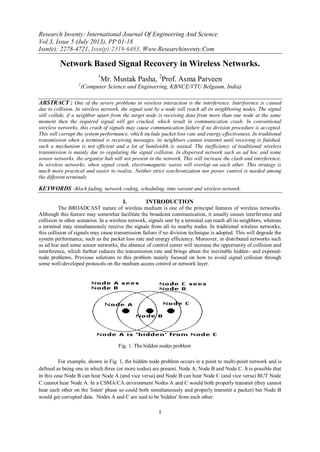
  • 1. Research Inventy: International Journal Of Engineering And Science Vol.3, Issue 5 (July 2013), PP 01-18 Issn(e): 2278-4721, Issn(p):2319-6483, Www.Researchinventy.Com 1 Network Based Signal Recovery in Wireless Networks. 1 Mr. Mustak Pasha, 2 Prof. Asma Parveen 1 (Computer Science and Engineering, KBNCE/VTU Belgaum, India) ABSTRACT : One of the severe problems in wireless interaction is the interference. Interference is caused due to collision. In wireless network, the signal sent by a node will reach all its neighboring nodes. The signal will collide, if a neighbor apart from the target node is receiving data from more than one node at the same moment then the required signal will get cracked, which result in communication crash. In conventional wireless networks, this crash of signals may cause communication failure if no division procedure is accepted. This will corrupt the system performance, which include packet loss rate and energy effectiveness. In traditional transmission when a terminal is receiving messages, its neighbors cannot transmit until receiving is finished, such a mechanism is not efficient and a lot of bandwidth is wasted. The inefficiency of traditional wireless transmission is mainly due to regulating the signal collision. In dispersed network such as ad hoc and some sensor networks, the organize hub will not present in the network. This will increase the clash and interference. In wireless networks, when signal crash, electromagnetic waves will overlap on each other. This strategy is much more practical and easier to realize. Neither strict synchronization nor power control is needed among the different terminals KEYWORDS -Block fading, network coding, scheduling, time variant and wireless network. I. INTRODUCTION The BROADCAST nature of wireless medium is one of the principal features of wireless networks. Although this feature may somewhat facilitate the broadcast communication, it usually causes interference and collision in other scenarios. In a wireless network, signals sent by a terminal can reach all its neighbors, whereas a terminal may simultaneously receive the signals from all its nearby nodes. In traditional wireless networks, this collision of signals may cause transmission failure if no division technique is adopted. This will degrade the system performance, such as the packet loss rate and energy efficiency. Moreover, in distributed networks such as ad hoc and some sensor networks, the absence of control center will increase the opportunity of collision and interference, which further reduces the transmission rate and brings about the inevitable hidden- and exposed- node problems. Previous solutions to this problem mainly focused on how to avoid signal collision through some well-developed protocols on the medium access control or network layer. For example, shown in Fig. 1, the hidden node problem occurs in a point to multi-point network and is defined as being one in which three (or more nodes) are present. Node A, Node B and Node C. It is possible that in this case Node B can hear Node A (and vice versa) and Node B can hear Node C (and vice versa) BUT Node C cannot hear Node A. In a CSMA/CA environment Nodes A and C would both properly transmit (they cannot hear each other on the 'listen' phase so could both simultaneously and properly transmit a packet) but Node B would get corrupted data. Nodes A and C are said to be 'hidden' from each other. Fig. 1. The hidden nodes problem
  • 2. Network Based Signal Recovery in Wireless … 2 The hidden nodes problem in wireless multi-hop sensor networks was mainly addressed with two techniques: RTS/CTS and Carrier Sense Tuning .RTS/CTS was basically designed to reduce the number of collisions due to hidden nodes by reserving the channel around both the sender and the receiver to protect frame transmission from being corrupted by hidden nodes. However, this method presents several problems when used in wireless multi-hop sensor networks: • The energy consumption related to a RTS/CTS exchange is significant, data frames are usually small, the collision probability is the same for data frames as for RTS/CTS, so it does not make any difference if the technique is used or not • It does not avoid collisions in multi-hop networks • It may lower the network capacity due to the exposed node problem, • It cannot be used for broadcast frames. Several MAC protocols have proposed to use Carrier Sense Tuning to cope with the hidden node problem .The key idea comes from the observation that hidden nodes cause Collisions, because their radio carrier sense range is not large enough to sense ongoing transmissions they may collide with. Hence, a node should tune its radio carrier sense range to make sure that when it transmits, there is no another transmission. Although this method allows a node to detect ongoing transmissions, it is not suitable for all situations. For example, it assumes a homogeneous radio channel for all nodes, which is not always possible because of obstacles, different antenna height, etc. Even if the channel is homogeneous, it is not possible to increase the carrier sense range of radio transceivers indefinitely due to physical limitations. 1.1 Use of RTS and CTS Hidden Nodes are solved by the use of a RTS (request to send)/CTS (clear to send) protocol prior to packet transmission. In our three node network above Node A sends a small RTS packet which is heard by Node B which send a small CTS packet which is heard by both Nodes A and Node C. Node C will not transmit in this case. 1.2 Node Identification Each node in a 802.11 network is identified by its MAC address (exactly the same as Ethernet a 6 byte - 48 bit value). Receiving nodes recognize their MAC address. A node wishing to send data initiates the process by sending a Request to Send frame (RTS). The destination node replies with a Clear To Send frame (CTS). Any other node receiving the RTS or CTS frame should refrain from sending data for a given time (solving the hidden node problem). The amount of time the node should wait before trying to get access to the medium is included in both the RTS and the CTS frame. This protocol was designed under the assumption that all nodes have the same transmission ranges. RTS/CTS are an additional method to implement virtual carrier sensing in Carrier sense multiple access with collision avoidance (CSMA/CA). By default, 802.11 rely on physical carrier sensing only which is known to suffer from the hidden node problem. RTS/CTS packet size threshold is 0–2347 octets. Typically, sending RTS/CTS frames does not occur unless the packet size exceeds this threshold. If the packet size that the node wants to transmit is larger than the threshold, the RTS/CTS handshake gets triggered. Otherwise, the data frame gets sent immediately. IEEE 802.11 RTS/CTS mechanism could help solve exposed node problem as well, only if the nodes are synchronized and packet sizes and data rates are the same for both the transmitting nodes. When a node hears an RTS from a neighbouring node, but not the corresponding CTS, that node can deduce that it is an exposed node and is permitted to transmit to other neighbouring nodes. If the Fig. 2. Use of RTS/CTS protocol prior to packet Transmission
  • 3. Network Based Signal Recovery in Wireless … 3 nodes are not synchronized (or if the packet sizes are different or the data rates are different) the problem may occur that the sender will not hear the CTS or the ACK during the transmission of data of the second sender. In this paper, we shall put forward some efficient signal recovery algorithms without the request of synchronization and power control among multiple data streams. Thus, the strategy is much more practical and easier to realize. With our proposed algorithms, since certain types of signal collision are allowed, the throughput and efficiency of wireless networks can greatly be increased. In different types of wireless channels, the waveforms of the received signals are different, thus requiring different algorithms to recover the useful signals. In this paper, we shall put forward several algorithms for three types of wireless channels. For additive white Gaussian noise (AWGN) and block-fading channels, where the attenuation is constant during the transmission of one frame, the recovering algorithms for BPSK and π/4-QPSK modulated signals will be developed, respectively, without loss of generality. For the time-variant channel, we must know the amplitude of the interference signal at each sampling time because the attenuation varies during the transmission of one frame. Two algorithms on signal recovery will be proposed for large and small coherent times, respectively. Simulation results will show that the bit error rate (BER) of the recovered signal using our developed schemes is almost the same as the transmission without interference, which proves the effectiveness of our strategy based on network coding. The rest of this paper is organized as follows: The network model and the scheduling strategy based on physical-layer network coding are discussed in Section II. In Section III, we will present the signal-recovery algorithms for AWGN and block-fading channels. In Section IV, two algorithms of signal recovery for time-variant channels will be put forward. The performance of the proposed strategy and some other practical issues are discussed in Section V. Section VI illustrates the simulation results, which demonstrate the effectiveness of our approach. Finally, we conclude this paper in Section VII. II. NETWORK MODEL AND THE SCHEDULING STRATEGY Our model of wireless networks is shown in Fig. 3, where the source terminals S1 and S2 intend to transmit two frames of messages x  = {x1, . . . , xL} and y  = {y1, . . . , yL} to the receivers R1 and R2, respectively. L is called the “frame length” here. The link between each pair of adjacent terminals is assumed to be half- duplex, which means that each terminal can both transmit and receive messages from its neighbors, but cannot simultaneously do them. Since R1 and R2 are both inside the transmission region of S1, x  can be received by the two receivers at the same time. If S1 and S2 simultaneously transmit, the signal of y  will collide with that of x  at R2, which may result in the transmission failure in traditional systems. However, if R2 knows the content of x  , it can eliminate the interference of x  and recover y  from the mixed signal. Each multi hop transmission session in wireless networks can well be described by this linear network model. In fact, the model shown in Fig. 3 is a special case. There may be multiple interference signals at R2. It will be shown that, as long as the receiver knows the information on all the interference signals, it can recover its desired signal through our algorithms with a very large probability. Fig. 3. Model of wireless networks with signal collision.
  • 4. Network Based Signal Recovery in Wireless … 4 For convenience, we only consider the scenario with just one interference signal when we develop the algorithms in the following sections. However, all these algorithms can easily be generalized to the multi- interference case. As mentioned in the previous section, the scheme on signal recovery depends on the channel property. In AWGN and block-fading channels, the attenuation is taken to be constant during the transmission of one frame. Thus, one only needs to estimate the delay and amplitude of the frame of interference signal, and then the interference signal can be “subtracted” from the mixed signal to recover the useful signal. The single- side power spectral density of the additive white noise is assumed to be N0/2. For the block-fading channel, the attenuation is assumed to be a Raleigh variable with a mean square value of 1, and different frames are assumed to suffer different and independent attenuations. However, in a general fading channel, if the attenuation varies during the transmission of one frame, we have to estimate the sampling value of each symbol in the frame of the interference signal. To develop an effective signal-recovery algorithm for time-variant channels, an appropriate channel model that can characterize different coherent times is needed. ARMA (p, q) process is a simple stochastic process model with the aforementioned property. It has been shown that for each random process, one can find an autoregressive moving average (ARMA) process such that its mean square error from the given process is as small as possible if p and q are large enough. The generating equation of an ARMA (p, q) process is qnqnnpnpnn vvAuAuA    ...... 1111 (1) where iA is the attenuation at the sampling time it , and i is a pure Gaussian random process with mean  and variance  2 . Without loss of generality, we assume that  = 0. Thus, iA is also a Gaussian random variable. Given pnn AA  ,...,1 and qnn   ,...,1 , the conditional normal distribution function of nA is ),...,,,...,|( 11 qnnpnnn AAzAp                          2 1 1 2 2 1 exp 2 1 p i q j jniini εε εvAuz σπσ =          2 2 2 1 exp 2 1 nAz   (2) where      p i q j jninin vAuA 1 11  is the conditional expectation value of nA . Since a Raleigh random variable is the sum of the squares of two Gaussian variables with mean 0 and the same variances, both the in- phase and quadrature attenuations of a Raleigh fading channel can be modeled by the ARMA processes. The coefficients  iu and  iv in (1) can be figured out through the channel estimation, and the values of p and q are chosen according to the tradeoff between the accuracy and complexity. If q = 0 in (1), the ARMA process is reduced to an autoregressive (AR) process ....12 npnpnn AuAuA   (3) The AR process is Markovian, which means that each An is only related to the former p attenuation values. Since the AR process is easier in form, we will only present the signal recovery algorithms for the channel modeled by the AR process in the latter part of this paper. For the general ARMA process, the algorithms and corresponding deductions are similar. Next, we will briefly discuss the scheduling strategy based on the signal-recovery algorithms. First, each terminal stores the frames it has recently received. Then, we add the identifier of the frame to be sent in the next time slot to the RTS message. Each frame has a unique identifier, which can be defined by the source address and the index of the frame. Thus, the terminal that receives the RTS messages from its neighbors can decide whether they can simultaneously transmit according to the identifier. If among all the frames to be sent there is only one unstored frame, the terminal will broadcast a CTS message; otherwise, the terminal will reply a non-CTS message with the identifiers of the frames that may cause unsolvable interference. Take, for example, in contrast to the traditional scheduling strategy, A is allowed
  • 5. Network Based Signal Recovery in Wireless … 5 to transmit b in time slot 3. Then, B will receive a mixed signal of a and b. Since B has received a before time slot 3, B can recover the data of b from the mixed signal through our algorithms developed later. In the next time slot, B can forward the recovered b to the next relay C. Node C will then receive the mixed signal of a and b in time slot 4 and recover b using the same method as before. In time slot 5, node A will transmit another frame of data, namely, c, and so on. It can be seen that if the data stream is incessant, it will take an average of two time slots to transmit one frame. Compared to with the one third frames per time slot in traditional scheduling, the throughput is significantly increased. 2.1 Network Block Codes Consider for a moment a simple unicast scenario shown in Fig.4 assume that the source is connected to the destination through h edge-disjoint paths each consisting of unit-capacity edges, and that any t of these edges can introduce errors. Note that an error can propagate only through the path on which it is introduced. Therefore, the receiver will observe at most t corrupted symbols, and the source can send information at rate k to the receiver by the means of an (h, k, 2t + 1) channel block code that maps k information symbols to h coded symbols, and can correct any t random errors. The coded symbols will be sent simultaneously on the h edges, thus using the “space” as the resource to accommodate for the redundancy introduced by the code, rather than time as in classical channel coding where coded symbols are sent sequentially and errors occur at different time slots. Consider now a multicast scenario where a source is connected to multiple receivers through an arbitrary network with the min-cut between the source and each receiver equal to h. Note that if different sets of h edge disjoint paths between the source and different receivers do not overlap, network coding is not necessary, and the problem reduces to that of Fig. 4 for each receiver separately, and thus to classical channel coding. Otherwise, we want to design the network code to protect the source message for each receiver. Fig. 4. Simple unicast scenario Definition. A network code is t-error correcting if it enables each receiver to correctly receive source information as long as the number of edges that introduce errors is smaller than t. Unlike classical channel codes, network error correction codes use coding operations not only at the source, but also at intermediate nodes of the network. Therefore, an error introduced at a single edge may propagate throughout the network. For simplicity we will assume that both the source and the channel (network) alphabet are Fq. Therefore, Fig. 4 at the source node, k information symbols are encoded into h coded symbols, which are then simultaneously transmitted to the destination. The source produces qk messages. If the network code is such that each receiver can correctly decode if errors are introduced in up to t edges, then, for each receiver, the set of qk h-dimensional vectors at any h-cut corresponding to the qk different source messages will be an (h, k) classical code that can correct at least t errors. Therefore, the appropriate channel coding bounds connecting parameters q, h, k, and t hold. 2.2 Bit Error Rate (BER): Bit error Rate, sometimes bit error ratio (BER) is the most fundamental measure of system performance. That is, it is a measure of how well bits are transferred end-to-end. While this performance is affected by factors such as signal-to-noise and distortion, ultimately it is the ability to receive information error- free that defines the quality of the link Bit error ratio (BER) is the number of bits received in error, divided by the total number of bits received. It is the percentage of bits that have errors relative to the total number of bits received in a transmission, usually expressed as ten to a negative power. For example, a transmission might have a BER of 10-5 , meaning that on average, 1 out of every of 100,000 bits transmitted exhibits an error. The BER is an indication of how often a packet or other data unit has to be retransmitted because of an error. If the BER is higher than typically expected for the system, it may indicate that a slower data rate would actually
  • 6. Network Based Signal Recovery in Wireless … 6 improve overall transmission time for a given amount of transmitted data since the BER might be reduced, lowering the number of packets that had to be resent. The formulae to calculate the BER are used here as follows: Case-I: In this case, AWGN is generated by using „randn‟ function and multiplied by noise power data sequence is generated by using „randsrc‟ function. Received data is obtained by adding AWGN and data bit generated earlier. „sign‟ function is used to demodulate and recover data in noisy condition. „abs‟ function is used to find absolute value and complex magnitude. Case-II: In this case, AWGN is generated by using „randn‟ function and multiplied by signal power data sequence is generated by using „randsrc‟ function and multiplied by signal power. Received data is obtained by adding AWGN and data bit generated earlier. „sign‟ function is used to demodulate and recover data in noisy condition and then multiplied by signal power. „abs‟ function is used to find absolute value and complex magnitude. To calculate the Bit Error Rate (BER): Err-symbol=abs(recover_data-TX_data) Total_err=length(find(Err_sysnbol)) BER=Total_err/N III. SIGNAL-RECOVERY ALGORITHM FOR AWGN AND BLOCK-FADING CHANNELS Additive white Gaussian noise (AWGN) is a channel model in which the only impairment to communication is a linear addition of wideband or white noise with a constant spectral density (expressed as watts per hertz of bandwidth) and a Gaussian distribution of amplitude. The model does not account for fading, frequency selectivity, interference, nonlinearity or dispersion. However, it produces simple and tractable mathematical models which are useful for gaining insight into the underlying behavior of a system before these other phenomena are considered. 3.1 Channel capacity The AWGN channel is represented by a series of outputs Yi at discrete time event index i. Yi is the sum of the input Xi and noise, Zi, where Zi is independent and identically distributed and drawn from a zero-mean normal distribution with variance n(the noise). The Zi are further assumed to not be correlated with the Xi. Zi ~ N(0,n) Yi = Xi + Zi ~ N(Xi, n) The capacity of the channel is infinite unless the noise n is nonzero, and the Xi is sufficiently constrained. The most common constraint on the input is the so-called "power" constraint, requiring that for a codeword (x1, x2, ……, xk) transmitted through the channel, we have:   k i i Px n 1 21 where P represents the maximum channel power. Therefore, the channel capacity for the power-constrained channel is given by: );(max)(..)( 2 YXIC PXEtsxf   Where f(x) is the distribution of X. Expand I(X;Y), writing it in terms of the differential entropy: I(X;Y) = h(Y) – h(Y|X) = h(Y) – h(X+Z|X) = h(Y) – h(Z|X) But X and Z are independent, therefore: I(X;Y) = h(Y) – h(Z) Evaluating the differential entropy of a Gaussian gives:
  • 7. Network Based Signal Recovery in Wireless … 7 )2log( 2 1 )( enZh  Because X and Z are independent and their sum gives Y: nPZEZEXEXEZXEYE  )()()(2)()()( 2222 From this bound, we infer from a property of the differential entropy that ))(2log( 2 1 )( nPeYh   Therefore the channel capacity is given by the highest achievable bound on the mutual information: )2log( 2 1 ))(2log( 2 1 );( ennPeYXI   Where I(X;Y) is maximized when: ),0(~ PNX Thus the channel capacity C for the AWGN channel is given by:        n P C 1log 2 1 3.2 Channel capacity and sphere packing Suppose that we are sending messages through the channel with index ranging from 1 to M, the number of distinct possible messages. If we encode the M messages to bits, then we define the rate R as: n M R log  A rate is said to be achievable if there is a sequence of codes so that the maximum probability of error tends to zero as n approaches infinity. The capacity C is the highest achievable rate. Consider a codeword of length n sent through the AWGN channel with noise level N. When received, the codeword vector variance is now N, and its mean is the codeword sent. The vector is very likely to be contained in a sphere of radius  Nn around the codeword sent. If we decode by mapping every message received onto the codeword at the center of this sphere, then an error occurs only when the received vector is outside of this sphere, which is very unlikely. Each codeword vector has an associated sphere of received codeword vectors which are decoded to it and each such sphere must map uniquely onto a codeword. Because these spheres therefore must not intersect, we are faced with the problem of sphere packing. How many distinct code words can we pack into our n-bit codeword vector? The received vectors have a maximum energy of n(P+N) and therefore must occupy a sphere of radius  NPn  . Each codeword sphere has radius nN . The volume of an n-dimensional sphere is directly proportional to rn , so the maximum number of uniquely decodable spheres that can be packed into our sphere with transmission power P is:       NP n n n nN NPn /1log 2 2 2 2    By this argument, the rate R can be no more than  NP /1log 2 1  . In the following section, we shall develop the signal-recovery algorithm in AWGN and block-fading channels. In the following discussion, we assume that each frame has L symbols and that the delay D of relative to y  is an integer and uniformly distributed on [−L, L]. In the following two parts, we will present the algorithms on recovering y  from the mixed signal yx   for BPSK and π/4 for QPSK modulations, respectively. For other types of linear modulation, the principle of the recovery algorithm is similar.
  • 8. Network Based Signal Recovery in Wireless … 8 3.3. Signal Recovery for BPSK Modulation For BPSK modulation, the signals of x  and y  can mathematically be written as Ax(t − D) cos(ωt + γ) and By(t) cos(ωt), respectively, where x(t), y(t) {1,−1}, and  is the phase shift of the carrier of x  from that of y  . A and B are the signal amplitudes of x  and y  , respectively. Thus, the mixed signal of x  and y  at node R2 can be represented by After demodulation and filtering, the sampled signal value of each symbol is where k is the sampling index, and nk is the additive Gaussian noise with variance σ2 n = N0/2. For simplicity, let yk = xk = 0 for k  [−L + 1, 0)  [L, 2L). We also assume that the carrier phase of y  and the local oscillator are ideally synchronized, and the impact of carrier-phase errors will be discussed later in Section V. Since the terminal R2 has received x  before, it can regenerate the sampling signal xk for 0 ≤ k < L. Then, one can compute the correlation between {sk} and the delayed signal {xk−d}, where d(−L,L) is an integer, to estimate A and D. That is where A’ = A cos γ. Through effective source coding and channel coding, xk and yk will take the value of {−1, 1} with equal probability and are independent of each other. Thus, we are satisfied that According to the law of large numbers, if the frame length L is sufficiently large,     12 / L Lk kk Ldxy and     12 / L Lk kk Ldxn will converge to 0 with very high probabilities. Moreover is valid with a probability close to 1. Therefore, if one computes  dxsR ,,  for each d (−L,L) and find out the maximum value, a reasonable estimation of A and D can be obtained by (8) where Dˆ = arg max−L<d<L  dxsR ,,  . By subtracting the estimated signal of x  from s  , y  can be recovered by (9)
  • 9. Network Based Signal Recovery in Wireless … 9 Note that if there are h frames of interference signals denoted by h xxx  ,...,, 21 instead of only one x  , all the interferences can be eliminated by repeating the aforementioned process for h times. Here is a simplified description of this algorithm. Algorithm 1: Signal-Recovery Algorithm for BPSK in AWGN and Block-Fading Channels. 3.4 Recovering Algorithm for π/4-QPSK Modulation π/4-QPSK modulation is widely used in wireless communications. For π/4-QPSK modulation, the input bit stream is partitioned by a serial-to-parallel converter into two parallel data streams mI,k and mQ,k, each with a symbol rate equal to half that of the incoming bit rate. Thus, we assume that the frame length is 2L symbols for convenience. Then, the signal of π/4-QPSK is given by (10) where kkk   1 , and  4/3,4/3,4/,4/  k is related to mI,k and mQ,k according to a certain mapping rule. Hence, the mixed signal at node B is where γ is the phase difference between the carriers of x  and y  . D is the delay of x  relative to y  , whereas B and A are the attenuations. Suppose that the phase shift of the local carrier from the carrier of y  is α. Then, after demodulation, the sampled in-phase and quadrature signals are respectively. nI,k and nQ,k are the Gaussian noises with mean 0. Similarly to BPSK, the sampled signal values of x  and y  are set to be 0 if k < 0 or k ≥ L. The principle of signal recovery is similar to that for BPSK, and we make use of the correlation between s(t) and x  . First, node R2 maps x  to   1 0   L Kxk according to the same rule at the transmitter. Then, let
  • 10. Network Based Signal Recovery in Wireless … 10 In (12a),   LnnB L Lk L Lk dxkkQdxk L Lk kIdxkyk /sincoscos 12 12 , 12 ,                 converges to 0 as L with a probability of 1. Moreover is valid with a probability of 1. Then, the estimated value of A cos(γ − α) is given by Similarly, one can estimate A sin(γ − α) from (12b) by In the preceding equations Hence, the interference of x  can be eliminated from the mixed signal s(t) as follows:
  • 11. Network Based Signal Recovery in Wireless … 11 Finally, one can decode ykIˆ , ykQˆ and recover the original data of y  through base band differential detection. Since this technique only computes 1 ykyk  for each k and the constant phase error α has no effect on the decoding result, phase synchronization is not required here. In the aforementioned two algorithms, the searching range of d is set to be (−L, L). In fact, it is not necessary to check all the values between −L and L. The start and end times of a frame can be found out through its head and tailing bits, respectively. Then, the length of the frame can be figured out. Although accurate duration of the mixed signal is difficult to detect, one can still get an approximate estimation. In addition, whether D >0 or D <0 can be decided by checking the identifier in the frame head. Thus, the searching range of d can greatly be shortened. For example, if we have detected D >0 and the duration of the mixed signal is quite probably between N − l/2 and N + l/2 symbols. Thus, the start time of x  is just L symbols before the termination time of the mixed signal, so D is probably between N − l/2 − L and N + l/2 − L. Therefore, one can only consider d [N − l/2 − L, N + l/2 − L], where l is a predefined parameter. The larger l is, the larger the probability of D [N − l/2 − L, N + l/2 − L] is. This way, the estimation of D will be more accurate, and the complexity can largely be reduced. IV. SIGNAL-RECOVERY ALGORITHM FOR TIME-VARIANT CHANNELS In time-variant channels, the attenuation is not constant during one frame; thus, we need to estimate the signal amplitude of each symbol of x  . However, if the channel slowly varies, the signal amplitude can still be estimated by calculating the correlation. An easy and reasonable way is to calculate the glide correlation between x  and s  . Suppose that the coherent time of the channel is the duration of M symbols. The signal amplitude Ai of xi can be worked out by calculating the local correlation value as For 2/2/ MLiM  . Then, let MRA ii /ˆ  be the estimated signal amplitude of xi. Here is the algorithm for BPSK. (For QPSK4/ and other types of modulations, the ideas are the same). Algorithm 2: Glide Correlation Algorithm on Signal Recovery for BPSK in Time Variant Channels. If the coherent time M is relatively small, Ai may not be accurately estimated through the correlation, and considerable interference may be induced. To deal with this problem, we will propose another signal-
  • 12. Network Based Signal Recovery in Wireless … 12 recovery algorithm based on maximum likelihood. Without loss of generality, we shall take BPSK as an example. The received mixed signal of x  and y  can be represented by (18) where B’k and yk are the amplitude and phase gains of the channel from S2 to R2 at the sampling time k, respectively. Similarly, Av’ and xk are the channel gains from S1 to R2. θyk and θxk are the binary phase shifts related to the information bits in x  and y  , respectively. Since θyk and θxk only have two possible values, namely, 0 and π, we have (19) In (19), the attenuations ykkB cos' and xkkA cos' are Gaussian random variables modeled by the AR processes. For simplicity, let Bk = ykkB cos' and Ak = xkkA cos' . Since Ak, Bk, and nk are independent of each other, the joint distribution of the three variables is where kB and kA are the expectations defined as (2), whereas x and y correspond to the variance  in (2). Note that maximizing the joint probability equates to minimizing the power part in (20). Hence, one only needs to solve the following optimization problem M: Let us normalize the variables in the objective function by setting   ,/ ~ xDkDkDk AAA     ,/ ~ ykkk BBB  and nkk nn /~  . Then, yk H can be regarded as the square of the Euclidean distance from  kkDk nBA ~, ~ , ~  to the origin. Let ;coscos' DkDxkkykkk ABss   thus, the solution to the problem M is as follows: After solving (21), one can compute 1kB and DkA 1 as in (2). Then, the amplitude of the signals of x  and y  , as well as the Gaussian noise, can recursively be figured out. Note that in (22), θyk is an unknown variable. Fortunately, θyk has only finite values. One can first calculate yk H for θyk = 0 and π, respectively, and then select θyk = arg min yk H as the decoding result of yk. Note that one needs to know the delay D before performing the recursive calculation. This can be achieved by the correlation method mentioned in Section III. Another problem is how to calculate the initial values of kAˆ and kBˆ for k ≤ p [p is the order of the AR process defined in (3)]. If D > 0, which means x  is sent later than y  , then the foreside of y  is not disturbed by x  . Since only the destroyed part of y  needs signal
  • 13. Network Based Signal Recovery in Wireless … 13 recovery, one can set the initial values ykkk sB cos/ˆ  for k ≤ p, whereas the initial values of kAˆ can be set to be 0. For D <0, the strategy is similar. In conclusion, the algorithm can be summarized as follows. Algorithm 3: Signal-Recovery Algorithm by Maximizing the Posterior Probability for BPSK in Time-Variant Channels. Considering the errors in the aforementioned estimation of the initial values of Ak and Bk, we will adopt the following method to improve the recovery result: First, Algorithm 3 is performed. Then, the obtained  kBˆ and  DkA  ˆ are regarded as the initial values of the attenuations. Take D > p, for example, and let the initial values xkkk sA cos/'  and 1 ˆ  Lk BB for L ≤ k < L+ p. Then, we calculate the attenuation values in reverse order from the sampling time min {L, L + D} to max {0, D} according to Algorithm 3. After that, we combine the two results and choose the one maximizing the likelihood. This method can make full use of the information in the signal and, thus, can enhance the performance of the algorithm with a relatively high complexity. Since the channel model in (1) is a forward generating equation, the inverted generating function needs to be derived for the reverse computation. Note that the function in (1) is essentially a conditional distribution of a Markovian process, and the joint distribution of multiple Gaussian random variables is still a Gaussian distribution characterized by the covariance matrix and the means of the variables. The inverted generating function can be obtained by calculating the co-variances between the attenuations at different sampling times. For the AR process, however, the problem can be simplified by the following proposition. Proposition 4.1: Given an AR process with mean 0 as in (3), the inverted generating function is where ζn is a purely random Gaussian process with mean 0 and variance 2  .
  • 14. Network Based Signal Recovery in Wireless … 14 V. PERFORMANCE ANALYSIS 5.1 Performance Analysis In the following section, we will analyze the performance of the recovery algorithms in the previous sections. Due to the complexity of time-variant channels, we will only derive the analytical results for AWGN and block-fading channels. The performance in time-variant channels will be shown by simulation results in the next section. We shall consider the BER performance and the effect of phase errors, as well as the inter symbol interference (ISI). 5.2.1 BER Performances First, we consider BPSK modulation. From the correlation algorithm of signal recovery in Section III- A, it can be seen that the resulting error bits in the recovered frame y  are mainly due to two factors, namely, the Gaussian noise and estimation errors of A and D. If Dˆ = D, then from (9) Thus, the total noise       1 ./' LD Dj kDjjDjjDkk nLxnxByxn Note that     1 / LD Dj DjjDk Lxnx is a Gaussian random variable with mean 0 and variance ./2 Ln According to the central limit theorem,     1 / LD Dj DjjDk Lxyx can be approximated by a Gaussian variable with mean 0 and variance   ./1/ 2 LLDL  Thus, the variance of kn' is smaller than .// 222 ' 2 LBLnnn   Thus the conditional BER satisfies. If L is large enough and the signal-to-noise ratio (SNR) of the channel is relatively small, the noise induced by the correlation operation has a little effect on the total SNR and the BER performance. Consider the probability  DDP ˆ subsequently. Suppose d [D − l/2, D + l/2], then Where ./)22( 2222 LBA nz   According to (25) and (26), given A, B, and ,2 n the upper bound of the BER is
  • 15. Network Based Signal Recovery in Wireless … 15 From (27), it can be seen that the larger L is, the better the BER performance is. If L is large enough, the noise induced by calculating the correlation can be neglected. For the block-fading channel, where A and B are random variables, the upper bound of the BER is given by where pA(A) and pB(B) are the Rayleigh distribution functions of A and B, respectively. The BER analysis of π/4- QPSK in AWGN and block-fading channels is similar to that of BPSK. It must also be noted that there may be error bits in x  itself, and this will impact  DDP ˆ and increase the BER of y  . Hence, it is necessary to adopt a reliable channel coding scheme to avoid the propagation of error bits. 5.2.2 Impact of the Synchronization Error Since the baseband differential detection technique only detects the phase difference between the previous and current samples, the constant phase shift α will not affect the demodulation result of π/4-QPSK. However, for BPSK, the phase error of the local carrier will reduce the power of the received signal and result in BER performance degradation. Assume that in (4), the phase difference between y  and the local carrier is y , and that between x  and the local carrier is x . After coherent demodulation, the sampled signal is After eliminating x  from the mixed signal s  , the power loss of y  is cos2 y . Suppose that y is uniformly distributed on [−π, π], then the average power loss is However, if differential PSK is adopted, the BER degradation due to the phase error is less than 1 dB for large SNRs. 5.2 Effects in time domain (time variant) In serial data communications, the AWGN mathematical model is used to model the timing error caused by random jitter (RJ). The graph to the right shows an example of timing errors associated with AWGN. The variable Δt represents the uncertainty in the zero crossing. As the amplitude of the AWGN is increased, the signal-to-noise ratio decreases. This results in increased uncertainty Δt. When affected by AWGN, The average number of either positive going or negative going zero-crossings per second at the output of a narrow band pass filter when the input is a sine wave is:
  • 16. Network Based Signal Recovery in Wireless … 16 Where  f0 = the center frequency of the filter  B = the filter bandwidth  SNR = the signal-to-noise power ratio in linear terms 5.2 Effects in phasor domain In modern communication systems, band limited AWGN cannot be ignored. When modeling band limited AWGN in the phasor domain, statistical analysis reveals that the amplitudes of the real and imaginary contributions are independent variables which follow the Gaussian distribution model. When combined, the resultant phasor's magnitude is a Rayleigh distributed random variable while the phase is uniformly distributed from 0 to 2π. The graph to the right shows an example of how band limited AWGN can affect a coherent carrier signal. The instantaneous response of the Noise Vector cannot be precisely predicted; however its time-averaged response can be statistically predicted. As shown in the graph, we confidently predict that the noise phasor will reside inside the 1σ circle about 38% of the time; the noise phasor will reside inside the 2σ circle about 86% of the time; and the noise phasor will reside inside the 3σ circle about 98% of the time. VI. SIMULATION RESULTS In this section, we will present the sample simulation results to further investigate the performance of the proposed signal recovery algorithms. In the simulation, we adopt the network model shown in Fig. 3, where y  is the desired information, and x  acts as the interference. The delay of x  relative to y  is uniformly distributed in [−L, L]. In block-fading channels, the amplitudes of y  and x  are set to be independent Rayleigh random variables with variance 1. In AWGN channels, the amplitude of y  is set to be constant 1 and that of x  is set to be a random variable uniformly distributed in [−1, 1]. Fig. 4 shows the matching probability  DDP ˆ versus different frame lengths for both BPSK and π/4-QPSK modulations in the AWGN channel. In this figure, we set d [−L, L]. It can be seen that  DDP ˆ increases as L becomes larger, which is consistent with the theoretical analysis. For the frame length L = 5000,  DDP ˆ is more than 95% for BPSK and 90% for π/4- QPSK. This matching probability is acceptable since most wireless frames are not very short. The mismatching cases mainly result from the fact that the amplitude of x  is too small. In these cases, x  brings about little interference to y  and, thus, can be treated as common noise. Note the matching probability for BPSK is larger than that for π/4-QPSK, and this is mainly because for BPSK, ykxk−D has only two possible values, namely, 1 and −1. Whereas for π/4-QPSK, cos(θyk−θxk−d−α) and sin(θyk−θxk−d−α) have eight possible values, respectively. Thus, the variance of R( s  , x  , d) (d  D) in (5) is much smaller than that in (12). Fig. 5 shows the probability  DDP ˆ under different SNRs. It can be seen that the power of noise has little impact on Fig. 9. Zero-Crossings of a Noisy Cosine
  • 17. Network Based Signal Recovery in Wireless … 17  DDP ˆ under large frame lengths and moderate SNRs. The uppermost curve is the result of the method mentioned in the last paragraph in Section III with l = 3, and the match probability is much larger than that with d [−L,L]. Figs. 6 and 7 illustrate the BER performance of the recovery algorithms under different SNRs for AWGN and block-fading channels, respectively. For BPSK modulation, SNR = ,/ 22 nB  where B is the amplitude of y  , and σ2n is the power of the additive white noise. For π/4-QPSK, we define SNR = ,/ 22 nB  where n 2  is the variance of both nI,k and nQ,k in (11). Note that this definition is different from the standard definition of SNR for π/4-QPSK; thus, there is a constant shift from the curves of π/4-QPSK to that of BPSK. In Fig. 6, the BER of the algorithm with small L is larger than that with big L under high SNRs. Moreover, the transmission without interference and that with interference but adopting our recovery algorithm have almost the same BER under low SNRs, even if L is as small as 100. Fig. 7 shows the similar result in Rayleigh block- fading channels. Thus, the two figures indicate that the algorithm will bring about little additional noise to the desired signal if L is not too small. Therefore, with a proper frame length, the transmission capacity can be approached by our strategy.
  • 18. Network Based Signal Recovery in Wireless … 18 Fig. 8 shows the BER performance of the two algorithms in Section IV in a time-variant channel. The star curve is for the scenario with no interference. The BER curves with circles and triangles are obtained through Algorithms 2 and 3, respectively. Here, we use an AR process An − 0.99An−1 = εn as the channel model. We set  nAVar = 10, and thus, σε = 1.41. Again, the delay  LLD , . Comparing the value of σε with  nAVar , one can see that the attenuation of the channel varies rather rapidly. From our simulation, the attenuation value changes from positive to negative within an average duration of about 20 symbols. From the simulation result it is show that our algorithms are able to remove almost all the interference. VII. CONCLUSION In this paper, we have proposed a signal-recovery scheme based on the physical-layer network coding, which can eliminate the interference signal and recover the useful information from the mixed signal. By this scheme, a new scheduling strategy, which allows a certain kind of signal collision without division techniques, can be realized, and the throughput in wireless networks can greatly be increased. We have developed the signal-recovery algorithms for AWGN, block-fading, and time-variant channels, respectively. For AWGN and block fading channels, we made use of the correlation between the known information and the received signals at the relay nodes to separate the desired signal from the mixed signal. For time variant channels, if the coherent time is large enough, a glide correlation operation can eliminate the interference signal. A key feature of the proposed physical layer network coding strategy is that neither synchronization nor power control among the different transmitters is needed, thus making it well suited for distributed networks. By making of Theoretical analysis and simulation results have shown that the signal-recovery algorithms can largely eliminate the interference from the mixed signal. REFERENCES [1] A. Bachir, D. Barthel, M. Heusse, and A. Duda, “Hidden nodes avoidance in wireless sensor networks,” in Proc. Int. Conf. Wireless Netw., Commun. Mobile Comput., Jun. 13–16, 2005, pp. 612–617 [2] Kaveh Pahlavan, “Wireless information networks examines sensor and mobile ad-hoc networks”, International journal of wireless information, ISSN: 1068-9605, 2010, J.No. 10776 [3] T. C. Keong, presented at the Ad hoc mobile wireless networks: Protocols Syst. Conf., 2002. [4] S. A. Aly and A. E. Kamal. Network protection codes against link failures using network coding. In Proc. Of IEEE 2008 Global Telecommunications Conference, Dec. 2008. [5] Morgan Kaufmann, “Wireless Communications and Networking”, Jul 28, 2010 [6] Jochen H. Schiller. “Mobile Communications”, Addison-Wesley, 2003 [7] Theodore S. Rappaport, “Wireless Communications – Principles and Practice”, Dorling Kindersley, 2009 [8] IETF “Mobile ad-hoc Networks (manet), http://www.ietf.org/html.charters/manet-charter.html [9] Wireless Networking and Mobile IP”, http://www.cse.wustl.edu/~jain/refs/wir_book.html [10] Wireless Networking – online references”, “Mobile multimedia and communication”, http://www.mobile3q.com/, http://www.wirelessadvisor.com. [11] Rober Spalding, “Storage Networks: The Complete Reference”, ISBN: 0072224762, McGraw-Hill/Osborne © 2003.