Lecture04
•
0 gefällt mir•301 views

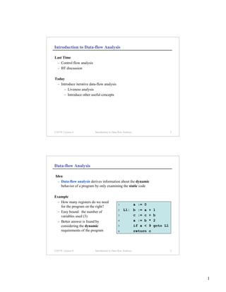
The document introduces data-flow analysis, which derives information about a program's dynamic behavior by examining its static code. It discusses liveness analysis, which determines whether a variable is live (will be used in the future) or dead at a given point. The concepts of control flow graphs, uses/defs, and solving the data-flow equations through iterative analysis are explained. An example liveness analysis is worked through to demonstrate the process.

Empfohlen
Empfohlen
Weitere ähnliche Inhalte
Was ist angesagt?
Was ist angesagt? (18)
Andere mochten auch
Ähnlich wie Lecture04
Ähnlich wie Lecture04 (15)
Mehr von sean chen
Mehr von sean chen (19)
Kürzlich hochgeladen
Kürzlich hochgeladen (20)
Lecture04
- 1. Introduction to Data-flow Analysis Last Time – Control flow analysis – BT discussion Today – Introduce iterative data-flow analysis – Liveness analysis – Introduce other useful concepts CIS570 Lecture 4 Introduction to Data-flow Analysis 2 Data-flow Analysis Idea – Data-flow analysis derives information about the dynamic behavior of a program by only examining the static code Example – How many registers do we need 1 a := 0 for the program on the right? 2 L1: b := a + 1 – Easy bound: the number of variables used (3) 3 c := c + b – Better answer is found by 4 a := b * 2 considering the dynamic 5 if a < 9 goto L1 requirements of the program 6 return c CIS570 Lecture 4 Introduction to Data-flow Analysis 3 1
- 2. Liveness Analysis Definition – A variable is live at a particular point in the program if its value at that point will be used in the future (dead, otherwise). ∴ To compute liveness at a given point, we need to look into the future Motivation: Register Allocation – A program contains an unbounded number of variables – Must execute on a machine with a bounded number of registers – Two variables can use the same register if they are never in use at the same time (i.e, never simultaneously live). ∴ Register allocation uses liveness information CIS570 Lecture 4 Introduction to Data-flow Analysis 4 Control Flow Graphs (CFGs) Simplification – For now, we will use CFG’s in which nodes represent program statements rather than basic blocks Example 1 a = 0 1 a := 0 2 b = a + 1 2 L1: b := a + 1 3 c := c + b 3 c = c + b 4 a := b * 2 5 if a < 9 goto L1 4 a = b * 2 6 return c 5 a<9 No Yes 6 return c CIS570 Lecture 4 Introduction to Data-flow Analysis 5 2
- 3. Liveness by Example What is the live range of b? – Variable b is read in statement 4, 1 a = 0 so b is live on the (3 → 4) edge – Since statement 3 does not assign 2 b = a + 1 into b, b is also live on the (2→ 3) edge 3 c = c + b – Statement 2 assigns b, so any value of b on the (1→2) and (5→ 4 a = b * 2 2) edges are not needed, so b is dead along these edges 5 a<9 No Yes b’s live range is (2→3→4) 6 return c CIS570 Lecture 4 Introduction to Data-flow Analysis 6 Liveness by Example (cont) Live range of a – a is live from (1→2) and again from 1 a = 0 (4→5→2) – a is dead from (2→3→4) 2 b = a + 1 Live range of b 3 c = c + b – b is live from (2→3→4) 4 a = b * 2 Live range of c – c is live from 5 a<9 (entry→1→2→3→4→5→2, 5→6) No Yes 6 return c Variables a and b are never simultaneously live, so they can share a register CIS570 Lecture 4 Introduction to Data-flow Analysis 7 3
- 4. Terminology Flow Graph Terms – A CFG node has out-edges that lead to successor nodes and in-edges that come from predecessor nodes – pred[n] is the set of all predecessors of node n 1 a = 0 succ[n] is the set of all successors of node n 2 b = a + 1 Examples – Out-edges of node 5: (5→6) and (5→2) 3 c = c + b – succ[5] = {2,6} – pred[5] = {4} 4 a = b * 2 – pred[2] = {1,5} 5 a<9 No Yes 6 return c CIS570 Lecture 4 Introduction to Data-flow Analysis 8 Uses and Defs Def (or definition) a = 0 – An assignment of a value to a variable – def[v] = set of CFG nodes that define variable v – def[n] = set of variables that are defined at node n a < 9? Use – A read of a variable’s value v live – use[v] = set of CFG nodes that use variable v – use[n] = set of variables that are used at node n ∉ def[v] More precise definition of liveness – A variable v is live on a CFG edge if ∈ use[v] (1) ∃ a directed path from that edge to a use of v (node in use[v]), and (2) that path does not go through any def of v (no nodes in def[v]) CIS570 Lecture 4 Introduction to Data-flow Analysis 9 4
- 5. The Flow of Liveness Data-flow – Liveness of variables is a property that flows through the edges of the CFG 1 a := 0 Direction of Flow – Liveness flows backwards through the CFG, 2 b := a + 1 because the behavior at future nodes 3 c := c + b determines liveness at a given node 4 a := b * 2 – Consider a – Consider b 5 a < 9? – Later, we’ll see other properties No Yes that flow forward 6 return c CIS570 Lecture 4 Introduction to Data-flow Analysis 10 program points Liveness at Nodes edges We have liveness on edges just before computation – How do we talk about a = 0 just after computation liveness at nodes? 1 a := 0 Two More Definitions – A variable is live-out at a node if it is live on anyb := a + 1 out- 2 of that node’s edges n 3 c := c + b live-out out-edges 4 a := b * 2 – A variable is live-in at a node if it is live on any of that < 9? in-edges 5 a node’s No Yes in-edges 6 return c live-in n CIS570 Lecture 4 Introduction to Data-flow Analysis 11 5
- 6. Computing Liveness Rules for computing liveness (1) Generate liveness: live-in If a variable is in use[n], n use it is live-in at node n (2) Push liveness across edges: pred[n] live-out live-out live-out If a variable is live-in at a node n then it is live-out at all nodes in pred[n] n live-in (3) Push liveness across nodes: If a variable is live-out at node n and not in def[n] live-in n then the variable is also live-in at n live-out Data-flow equations (1) in[n] = use[n] ∪ (out[n] – def[n]) (3) out[n] = ∪ in[s] (2) s ∈ succ[n] CIS570 Lecture 4 Introduction to Data-flow Analysis 12 Solving the Data-flow Equations Algorithm for each node n in CFG in[n] = ∅; out[n] = ∅ initialize solutions repeat for each node n in CFG in’[n] = in[n] save current results out’[n] = out[n] in[n] = use[n] ∪ (out[n] – def[n]) solve data-flow equations out[n] = ∪ in[s] s ∈ succ[n] until in’[n]=in[n] and out’[n]=out[n] for all n test for convergence This is iterative data-flow analysis (for liveness analysis) CIS570 Lecture 4 Introduction to Data-flow Analysis 13 6
- 7. Example 1st 2nd 3rd 4th 5th 6th 7th node use def in out in out in out in out in out in out in out # 1 a := 0 1 a a a ac c ac c ac c ac 2 a b a a bc ac bc ac bc ac bc ac bc ac bc 2 b := a + 1 3 bc c bc bc b bc b bc b bc b bc bc bc bc 4 b a b b a b a b ac bc ac bc ac bc ac 3 c := c + b 5 a a a a ac ac ac ac ac ac ac ac ac ac ac 6 c c c c c c c c 4 a := b * 2 Data-flow Equations for Liveness 5 a < 9? No Yes in[n] = use[n] ∪ (out[n] – def[n]) 6 return c out[n] = ∪ in[s] s ∈ succ[n] CIS570 Lecture 4 Introduction to Data-flow Analysis 14 Example (cont) Data-flow Equations for Liveness in[n] = use[n] ∪ (out[n] – def[n]) 1 a := 0 out[n] = ∪ in[s] 2 b := a + 1 s ∈ succ[n] 3 c := c + b Improving Performance out[3] Consider the (3→4) edge in the graph: in[4] 4 a := b * 2 out[4] out[4] is used to compute in[4] in[4] is used to compute out[3] . . . 5 a < 9? So we should compute the sets in the No Yes order: out[4], in[4], out[3], in[3], . . . 6 return c The order of computation should follow the direction of flow CIS570 Lecture 4 Introduction to Data-flow Analysis 15 7
- 8. Iterating Through the Flow Graph Backwards 1st 2nd 3rd node use def out in out in out in 1 a := 0 # 6 c c c c 2 b := a + 1 5 a c ac ac ac ac ac 4 b a ac bc ac bc ac bc 3 c := c + b 3 bc c bc bc bc bc bc bc 2 a b bc ac bc ac bc ac 4 a := b * 2 1 a ac c ac c ac c 5 a < 9? Converges much faster! No Yes 6 return c CIS570 Lecture 4 Introduction to Data-flow Analysis 16 Solving the Data-flow Equations (reprise) Algorithm for each node n in CFG in[n] = ∅; out[n] = ∅ Initialize solutions repeat for each node n in CFG in reverse topsort order in’[n] = in[n] Save current results out’[n] = out[n] out[n] = s ∈ succ[n] in[s] ∪ Solve data-flow equations in[n] = use[n] ∪ (out[n] – def[n]) until in’[n]=in[n] and out’[n]=out[n] for all n Test for convergence CIS570 Lecture 4 Introduction to Data-flow Analysis 17 8
- 9. Time Complexity Consider a program of size N – Has N nodes in the flow graph (and at most N variables) – Each live-in or live-out set has at most N elements – Each set-union operation takes O(N) time – The for loop body – constant # of set operations per node – O(N) nodes ⇒ O(N2) time for the loop – Each iteration of the repeat loop can only make the set larger – Each set can contain at most N variables ⇒ 2N2 iterations Worst case: O(N4) Typical case: 2 to 3 iterations with good ordering & sparse sets ⇒ O(N) to O(N2) CIS570 Lecture 4 Introduction to Data-flow Analysis 18 More Performance Considerations Basic blocks – Decrease the size of the CFG by merging nodes 1 a := 0 that have a single predecessor and a single successor into basic blocks b := a + 2 1 (requires local analysis before and after global c := c + 1 analysis) 3 a := b * c c + 2 b a > 9? One variable at a time 4 No := b * a 2 Yes – Instead of computing data-flow information return c 3 for all variables at once using sets, 5 a < 9? compute a (simplified) analysis for No Yes each variable separately 6 return c Representation of sets – For dense sets, use a bit vector representation – For sparse sets, use a sorted list (e.g., linked list) CIS570 Lecture 4 Introduction to Data-flow Analysis 19 9
- 10. Conservative Approximation X Y Z node use def in out in out in out # 1 a := 0 1 a c ac cd acd c ac 2 a b ac bc acd bcd ac b 2 b := a + 1 3 bc c bc bc bcd bcd b b 4 b a bc ac bcd acd b ac 3 c := c + b 5 a ac ac acd acd ac ac 6 c c c c 4 a := b * 2 Solution X 5 a < 9? – Our solution as computed on No Yes previous slides 6 return c CIS570 Lecture 4 Introduction to Data-flow Analysis 20 Conservative Approximation (cont) X Y Z node use def in out in out in out # 1 a := 0 1 a c ac cd acd c ac 2 a b ac bc acd bcd ac b 2 b := a + 1 3 bc c bc bc bcd bcd b b 4 b a bc ac bcd acd b ac 3 c := c + b 5 a ac ac acd acd ac ac 6 c c c c 4 a := b * 2 Solution Y 5 a < 9? – Carries variable d uselessly around the No Yes loop 6 return c – Does Y solve the equations? – Is d live? – Does Y lead to a correct program? Imprecise conservative solutions ⇒ sub-optimal but correct programs CIS570 Lecture 4 Introduction to Data-flow Analysis 21 10
- 11. Conservative Approximation (cont) X Y Z node use def in out in out in out # 1 a := 0 1 a c ac cd acd c ac 2 a b ac bc acd bcd ac b 2 b := a + 1 3 bc c bc bc bcd bcd b b 4 b a bc ac bcd acd b ac 3 c := c + b 5 a ac ac acd acd ac ac 6 c c c c 4 a := b * 2 Solution Z 5 a < 9? – Does not identify c as live in all cases No Yes – Does Z solve the equations? 6 return c – Does Z lead to a correct program? Non-conservative solutions ⇒ incorrect programs CIS570 Lecture 4 Introduction to Data-flow Analysis 22 The Need for Approximations Static vs. Dynamic Liveness – In the following graph, b*b is always non-negative, so c >= b is always true and a’s value will never be used after node 2 1 a := b * b Rule (2) for computing liveness – Since a is live-in at node 4, it is live-out 2 c := a + b at nodes 3 and 2 – This rule ignores actual control flow 3 c >= b? No Yes 4 return a 5 return c No compiler can statically know all a program’s dynamic properties! CIS570 Lecture 4 Introduction to Data-flow Analysis 23 11
- 12. Concepts Liveness – Use in register allocation – Generating liveness – Flow and direction – Data-flow equations and analysis – Complexity – Improving performance (basic blocks, single variable, bit sets) Control flow graphs – Predecessors and successors Defs and uses Conservative approximation – Static versus dynamic liveness CIS570 Lecture 4 Introduction to Data-flow Analysis 24 Next Time Lecture – Generalizing data-flow analysis CIS570 Lecture 4 Introduction to Data-flow Analysis 25 12