SlideShare ist ein Scribd-Unternehmen logo
1 von 39
Downloaden Sie, um offline zu lesen
Ertek, G., Incel, B. and Arslan, M. C. (2007). "Impact of Crossaisles in a rectangular warehouse: A
computational study," in Facility Logistics: Approaches and Solutions to Next Generation
Challenges, Editor: Maher Lahmar. Auerbach.

Note: This is the final draft version of this paper. Please cite this paper (or this final draft) as
above. You can download this final draft from http://research.sabanciuniv.edu.


               Impact of Cross Aisles in a Rectangular Warehouse:
                             A Computational Study


                         Gürdal Ertek, Bilge Incel, and Mehmet Can Arslan


                            Faculty of Engineering and Natural Sciences
                                          Sabanci University
                                           Istanbul, Turkey
Impact of Cross Aisles in a Rectangular Warehouse: A Computational Study


                                          Gürdal Ertek 1
                                        Sabancı University
                           Faculty of Engineering and Natural Sciences
                             Orhanlı, Tuzla, 34956, Istanbul, Turkey
                                     ertekg@sabanciuniv.edu

                                          Bilge Incel
                                           Roketsan
                                Ankara-Samsun Karayolu 40. Km
                                06780, Elmadağ, Ankara, Turkey
                                     b_incel@yahoo.com

                                       Mehmet Can Arslan
                                       Sabancı University
                           Faculty of Engineering and Natural Sciences
                             Orhanlı, Tuzla, 34956, Istanbul, Turkey
                                  mehmeta@su.sabanciuniv.edu


                                           Abstract
Order picking is typically the most costly operation in a warehouse and traveling is
typically the most time consuming task within order picking. In this study we focus on
the layout design for a rectangular warehouse, a warehouse with parallel storage blocks
with main aisles separating them. We specifically analyze the impact of adding cross
aisles that cut storage blocks perpendicularly, which can reduce travel times during order
picking by introducing flexibility in going from one main aisle to the next. We consider
two types of cross aisles, those that are equally spaced (Case 1) and those that are
unequally spaced, which respectively have equal and unequal distances among them. For
Case 2, we extend an earlier model and present a heuristic algorithm for finding the best
distances among cross aisles. We carry out extensive computational experiments for a
variety of warehouse designs. Our findings suggest that warehouse planners can obtain
great travel time savings through establishing equally spaced cross aisles, but little
additional savings in unequally-spaced cross isles. We present a look-up table that
provides the best number of equally spaced cross aisles when the number of cross aisles
(N) and the length of the warehouse (T) are given. Finally, when the values of N and T are
not known, we suggest establishing three cross aisles in a warehouse.

Keywords: warehouse design, warehouse layout, order picking, cross aisles, rectangular
warehouse.


1
    Corresponding author
                                               1
1. Introduction

       Order picking is generally the most significant operation in a warehouse,

accounting for approximately 60% of all operational costs in a typical warehouse

(Frazelle, 2001, page 147). Cost of order picking is affected by the decisions regarding

the facility layout and the selection of storage and retrieval systems, and by the

implemented strategies such as zoning, batching and routing. Travel cost is typically the

largest cost component within order picking, accounting for about 50% of the costs

associated with order picking activities (Frazelle and Apple, 1996). Since order picking,

specifically traveling, is costly, reducing the travel time spent for order picking can

significantly reduce operational costs.


Figure 1. Case 0: A rectangular warehouse with four storage blocks, five main aisles, and

no cross aisles (The vectors show a route to pick an order with seven items).


       In this chapter, we present the findings of a study that focuses on the strategic

layout decisions of how many cross aisles to establish within a rectangular warehouse

and how to determine the distances among them. A rectangular warehouse can be


                                              2
defined as a warehouse with equi-length parallel storage blocks, separated by aisles in

between (Figure 1). A sub-region of a large warehouse where routing decisions are made

independently from the remaining regions can also be considered as a rectangular

warehouse, given that it satisfies the structural properties described above. A rectangular

warehouse may have only main aisles which separate the storage blocks vertically

(Figure 1), or may also contain one or more cross aisles perpendicular to the main aisles,

which divide the storage blocks horizontally (Figures 2, 3 and 4). The main advantage of

cross aisles is that they enable savings in travel times, especially during the order picking

operations. Figures 1 and 2 illustrate an example of a rectangular warehouse where the

creation of a cross aisle can reduce the travel distance while picking an order with seven

items: The addition of the cross aisle (Figure 2) shortens the travel distance by enabling

shortcuts from the 5th main aisle to the 4 th main aisle and from the 4th main aisle to the 3rd

main aisle.


Figure 2. The warehouse displayed in Case 0 with an interior cross aisle with shortcuts

linking main aisle 5 to main aisle 4 and main aisle 4 to main aisle 3.


                                               3
Storage blocks typically consist of steel racks that are installed on the warehouse

floor permanently during the construction of a warehouse. Thus the decisions regarding

the quantities and dimensions of storage blocks, main aisles and cross aisles are strategic

decisions. These decisions should be made considering many factors, including:

      The physical dimensions of the building.

      The characteristics of the materials to be stored, including physical dimensions,

       weights, shelf lives, pallet sizes and projected demand patterns.

      The characteristics of warehouse equipment such as forklifts and AGVs.

      The quantity and capabilities of the workforce.

      The capabilities of the information system; i.e., the Warehouse Management

       System (WMS).

       One classic challenge raised by these factors is how to incorporate the interactions

between different decision levels in the design and operation of warehouses

(Rouwenhorst et al., 2000). For example, the strategic decision of determining the best

warehouse layout, the tactical decision of assigning the products to the storage locations

in the best way, and the operational decision of determining the best order picking routes

are all interdependent. In our study we assume that the widths of the storage blocks, the

main aisles and the cross aisles are fixed, and that the items stored in the warehouse all

have the same demand frequencies. Even under these simplifying assumptions, the

strategic decisions regarding the number of cross aisles and the distances between them

(the lengths of storage blocks) have to be made by estimating the average travel distance

in order picking under a specific routing algorithm. Hence, in our study we assume that


                                             4
the routing algorithm and the storage locations of products are pre-determined, and focus

on the strategic decisions regarding cross aisles.


Figure 3. A rectangular warehouse with equally spaced cross aisles (Case 1).


Figure 4. A rectangular warehouse with unequally spaced cross aisles (Case 2).


                                              5
For a rectangular warehouse, one can identify the following three cases with

respect to the number of cross aisles N and the distances in between them:

        Case 0: Warehouse with no cross aisles (N=0), as shown in Figure 1.

        Case 1: Warehouse with N equally spaced cross aisles (N1), as shown in Figure

         3.

        Case 2: Warehouse with N unequally spaced cross aisles (N1), as shown in

         Figure 4.

         In our study we seek answers to the following research questions regarding the

rectangular warehouse:

   1. Should the cross aisles be established equally spaced (Case 1) or unequally spaced

         (Case 2)? In other words, should the storage blocks have an equal length or

         variable lengths?

   2. How much travel time savings do cross aisles bring? Under which settings do

         cross aisles bring the most travel time savings?

   3. How many cross aisles should there ideally be in a rectangular warehouse? In

         other words, what is the best number of cross aisles?

         To answer these questions, we carry out extensive computational experiments

reflecting a variety of warehouse settings with different values for warehouse lengths (T),

number of cross aisles (M), and pick densities (D). Based on a thorough analysis of our

experimental results, we come up with solid answers to the research questions posed

above.

         One unique aspect of our research is that we extensively apply the starfield

visualization technique from the field of information visualization. In starfield


                                              6
visualization, various fields of a dataset are mapped to the axes of a colored 2-D or 3-D

scatter plot, and to the attributes of the glyphs (data points) such as color, size, and shape.

Information visualization is the growing field of computer science that combines the

fields of data mining, computer graphics, and exploratory data analysis (in statistics) in

pursuit of visually understanding data (Keim 2002, Spence 2001). The ultimate goal in

information visualization is to discover hidden patterns and gain actionable insights

through a variety of -possibly interactive- visualizations.

          The use of a visualization approach in the analysis of our numerical results will

enable us to make important observations, and develop managerial insights. To the best

of our knowledge, this is the first attempt where data/information visualization techniques

are employed to this extent in the warehousing and facility logistics literature.


2. Related Literature

          Rouwenhorst et al. (2000) present a reference framework and classification of

warehouse design and operating problems. Van den Berg and Zijm (1999) provide

another review of the warehousing literature that classifies warehouse management

problems. Sharp (2000) summarizes functional warehouse operations, database

considerations, and tactical, strategic and operational issues in warehouse planning and

design.

          Within the vast facility logistics literature, there exists studies that solely focus on

order picking routing and order batching for the purpose of reducing travel time. An early

study by Ratliff and Rosenthal (1983) solves for the routing problem in order picking.

Based on the number of aisles, the authors propose an algorithm that solves the problem


                                                 7
to optimality. They state that the algorithm computation time grows linearly in the

number of aisles, and is thus scalable for solving real world problems.

       Roodbergen and De Koster (2001) analyze the relationship between warehouse

layout and average travel time. They consider a rectangular warehouse in which a single

cross aisle divides the warehouse into two equal length blocks. The authors present a

dynamic programming algorithm to determine the shortest order picking routes, and show

that the addition of the cross aisle decreases average order picking time significantly.

       In another study, Roodbergen and De Koster (2001) compare several algorithms

for routing order pickers in a warehouse with more than one cross aisle. They introduce

two new heuristics, combined and combined+, and compare them with the S-Shape,

Largest Gap and Aisle-by-Aisle heuristics in the literature. The authors prove through

computational tests that the combined+ heuristic performs best among the five heuristics.

A branch-and-bound algorithm is used as a benchmark to compare the performances of

the generated heuristics.

       De Koster et al. (1999) report a real world application, where they significantly

improve the efficiency of manual order picking activities at a large retail distribution

center in Netherlands. In the first stage of their study, the authors apply a routing

heuristic, which ensures that order pickers pick items from both sides of an aisle. This

heuristic alone achieves a 30% reduction in travel time, and consequently a saving of 1.2

order pickers. In the latter stage of their study the authors apply order batching, time-

savings method and a combined routing heuristic (De Koster and Van der Poort 1998)

jointly, and achieve 68% reduction in travel distance and a saving of 3 to 4 pickers. This


                                              8
study is the perfect example of how the order picking strategies and routing algorithms

proposed in the literature can be applied in the real world to achieve substantial savings.

       Our study is mainly related to the work of Vaughan and Petersen (1999), who

consider both layout and routing. Vaughan and Petersen are motivated by the fact that

cross aisles can reduce travel distances due to their flexibility in order picking. The

authors develop a shortest path pick sequencing model that is applicable to any number of

equally spaced cross aisles (equal length storage blocks) in the warehouse. Their model

assumes that all the items along an aisle are picked before proceeding to the next aisle,

and the order picking progresses from the leftmost aisle to the rightmost aisle. This policy

is referred to as aisle-by-aisle policy. The authors compute the optimal routes for a large

number of randomly generated picking requests, over a variety of warehouse layout and

order picking parameters. Their results suggest that when the main storage aisle length

(T) is small, an excessive number of cross aisles can increase the average travel distance.

This is true especially when the number of storage aisles (M) is small, and when pick

density is very small or very large. The authors warn that the savings due to cross aisles

diminish, even turn into losses, if the number of cross aisles becomes excessive. This is

because the extra distance to traverse the cross aisles increases the travel distances.

Additionally, the authors find out that as the main storage aisle length (T) increases the

optimal number of cross aisles also increases and report that cross aisles are most

beneficial for longer warehouses.


                                              9
3. The Vaughan and Petersen Model

Vaughan and Petersen (1999) assume certain characteristics with respect to the

rectangular warehouses and order picking policies. Since our study is built on their

model, which we will refer to as the V&P model, these assumptions are also valid for our

model:

        There are parallel main aisles and products are stored on both sides of the main

         aisles.

        Each order includes a number of items to be picked, which are generally located

         in various main aisles.

        All stocks of a particular item are stored in a single location.

        Order pickers can traverse the aisles in both directions and change directions

         within the main aisles.

        The main aisles are narrow enough to pick from both sides of the aisle without

         changing position.

        The main aisles are wide enough such that two or more order pickers can operate

         in the main aisle at the same time.

        There are two natural cross aisles in the warehouse, at the head and rear of the

         warehouse.

        Cross aisles are not used to store items; they are only used to pass to the next

         main aisle.

        The items of an order are collected in a single tour.

         Block lengths are determined by the locations of the cross aisles that divide main

aisles perpendicularly. In our study, the number of cross aisles refers to the number of


                                               10
interior cross aisles, which are between the default head and rear cross aisles. We

 assume that picking routes start and end at the southeast and southwest corners of the

 warehouse, respectively. Even though some research assumes that order picking ends at

 the starting point (De Koster and Van der Poort 1998, Roodbergen and De Koster 2001),

 this does not make a great change in travel distance (and thus travel time). Petersen

 (1997) notes that this change results in at most 1% deviation in travel distance.


                      (a)                                           (b)

Figure 5. (a) A warehouse with storage blocks of equal lengths and (b) a warehouse with

storage blocks with unequal lengths (Arrows represent the total vertical travel distance to

pick items in main aisle m when the main aisle is entered from the ith cross aisle and left

from the jth cross aisle).


        The dynamic programming algorithm developed by Vaughan and Petersen (1999)

finds the optimal route to pick an order under the aisle-by-aisle policy. The complete

notation for their so called shortest path model is as follows:

L: Length of a storage block.

T: Length of the warehouse (equal to the length of main aisles), T   N  1L .

                                             11
M: Number of main aisles.

N: Number of interior cross aisles (The total number of cross aisles is N+2).

A: Width of a cross aisle. This parameter is essential for the calculation of the best aisle-

by-aisle route. The model assumes that an order picker walks along the center of the cross

aisles. This walking pattern is illustrated in Figure 5 and the additional distance of A/2 to

walk to the middle of the cross aisle is reflected in the formulas for B1m and B2 m.

B: Width of a main aisle.

C: Width of a storage block.

The notation until now is related to the warehouse layout. The notation below is given for

to a particular order to be picked:

Km: The number of items to be picked by the order picker from main aisle m = 1, 2, .., M.

                                      M
        Thus the order consists of    K
                                      m 1
                                             m   items in total.


Xm(t): The location of an item t in main aisle m = 1, 2, …, M, and t = 1, 2, …, K m

        (undefined if Km = 0) where 0  Xm(t)  T.

(The expressions listed below are demonstrated in Figure 5a.)

Xm+: The location of the item at the south-most location (highest value) in main aisle m

        (undefined if Km = 0), i.e. Xm+ = max  X m (t ) .
                                                     t


Xm-: The location of the item at the north-most location (smallest value) in main aisle m

        (undefined if Km = 0), i.e. Xm- = min  X m (t ) .
                                                 t


Cm(i,j): The total vertical travel distance required to pick all the items in main aisle m, if

        main aisle m is entered at cross aisle i and exited to main aisle m-1 at cross aisle j.


                                                         12
B1m(i,j): The length of forward-tracking leg required to pick the items in main aisle m to

        the north of cross aisle h, h = min (i,j).

B2m(i,j): The length of back-tracking leg required to pick the items in main aisle m to the

        south of cross aisle h, h = max (i,j).

fm(i): The minimum total picking distance required to pick all the items in aisle m, m-1,

        m-2, ..., 2, 1 if main aisle m is entered at cross aisle position i.

        In the V&P model Cm, B1m, and B2m are calculated as follows:

           C m (i , j )  B1m (i, j )  i  j ( L  A)  B 2 m (i , j ) ; where

                                         0                                               for             K m  0,
                                                                                                 
B1m (i , j )                            0                                               for    X  min(iL, jL),
                                                                                                  m

                
               2 min(iL, jL)  X   A(0.5  ((min(iL, jL)  X  ) / L))
                                  m                             m                        for     
                                                                                                 X  min(iL, jL);
                                                                                                  m

and

                                           0                                              for             K m  0,
                                                                                                     
B 2 m (i , j )                            0                                              for    X  max(iL, jL ),
                                                                                                      m

                 
                 2 max(iL, jL )  X  A(0.5  (( X   max(iL , jL )) / L))
                 
                                    
                                    m               m                                     for        
                                                                                                  X  max(iL, jL ).
                                                                                                      m


        The dynamic programming equations for each stage are given as follows:

fm (i)  min Cm (i, j )  f m1 ( j ) , where f1 (i )  C1 (i , N  1) .
            j


        Stages of the dynamic programming are related to the main aisle numbers in the

warehouse. The desired shortest-path picking route is determined by evaluating

f M ( N  1) .


4. The Modified Model

Now we present our model that allows us to find the best routes according to the aisle-by-

aisle heuristic for the case of unequally-spaced cross aisles (Case 2). The primary

                                                      13
difference between our model and the V&P model is that the storage blocks now have

variable lengths Li (Figure 5b) instead of a fixed length of L (Figure 5a) where Li is the

length of the ith storage block for i = 1,…, N+1. Thus, the length of the warehouse T

                                                                                     N 1
which is equal to the length of the main aisles can be expressed as T   Li .
                                                                                     i 1


Next, we define two new notations that give us the indices of the blocks where the north-

most and south-most items within an aisle are located:

Blockof(Xm+): Index of storage block Li in main aisle m where Xm+ is located for i = 1, 2,

…, N+1.

Blockof(Xm-): Index of storage block Li in main aisle m where Xm- is located for i = 1, 2,

…, N+1.

         Finally, the Cm, B1m and B2m values are calculated based on the modified

definitions of block lengths Li and the warehouse length T which can be expressed as:

                                 max( i , j )
Cm (i, j )  B1m (i , j )          
                              s  min( i , j ) 1
                                                    Ls  i  j A  B 2m (i , j ) ,


where

                       i      j                                                   
B1m (i, j )  2  min( Ls ,  L f )  X   A(0.5  min(i, j )  Blockof ( X  ))  , and
                                         m                                    m
                
                     s 1   f 1                                                  
                                                                                   

                               i      j                                                 
B 2m (i , j )  2  X   max( Ls ,  L f )  A(0.5  Blockof ( X  )  1  max(i, j )) 
                      m                                            m
                  
                             s 1   f 1                                                
                                                                                         


5. Algorithms to Identify Best Storage Block Lengths Li

         Given T, M, N, A, B, C and D values, the problem of finding the best storage

block lengths Li is a difficult problem. This is because the length of a tour is found by


                                                                     14
solving a dynamic programming problem and the locations of the items are uniformly

distributed. The objective function to be minimized is the average travel distance (and

thus, the average travel time) over all orders, with the optimal travel distance for each

order computed through dynamic programming optimization. We thus develop and

implement two heuristic search algorithms, namely GSA (Grid Search Algorithm) and

RGSA (Refined Grid Search Algorithm), to find the best Li values. GSA takes a

warehouse (with its T, M, N, A, B, C values), a set of generated orders and the number of

grids as parameters, and identifies an initial solution, which consists of Li values. RGSA

takes the solution of GSA as the initial solution and carries out a search to reduce the

average travel distance (i.e., average travel time). These algorithms are given in pseudo-

code and are explained in the Appendix.


Table 1. Experimental design.

                Factor                               Number of values   Values

                Length of main aisles (T) (meters)          6           30, 60, 90, 120, 150, 180
396 scenarios


                Number of main aisles (M)                   6           5, 10, 15, 20, 25, 30

                Pick density (D)                           11           0.1, 0.5, 1.0, 1.5, 2.0,

                (items/aisle)                                           2.5, 3.0, 3.5, 4.0, 4.5, 5.0

                Number of cross aisles (N)            1 (for Case 0)    0

                                                      8 (for Case 1)    1, 2, 3, 4, 5, 6, 7, 8

                                                      3 (for Case 2)    1, 2, 3

                (A, B, C) * (meters)                        1           (2.50, 1.25, 1.25)

*: A: Width of a cross aisle; B: Width of a main aisle; C: Width of a storage block


                                                     15
6. Experimental Design

       The different values of model parameters that we have used in our computational

experiments are depicted in Table 1. We investigate 396 scenarios (problem instances)

corresponding to 396 combinations of the warehouse length (T), the number of aisles (M)

and the pick density (D). In all these scenarios, the A, B, C parameters are respectively set

to fixed values of 2.50, 1.25 and 1.25 (meters).


Figure 6. Savings with respect to the pick density (D).


       One fundamental parameter is the pick density (D), which is the average number

of items per main aisle. In each scenario, the total number of items to be picked is

calculated as the multiplication of the pick density (D) with the number of main aisles

(M). The 11 pick density values listed above are used for calculating the order sizes

during the estimation of average route length for each scenario. Thus the 11 order sizes


                                             16
used in the experiments are 0.1M, 0.5M, 1.0M, 1.5M, 2.0M, 2.5M, 3.0M, 3.5M, 4.0M,

4.5M and 5.0M.


Figure 7. Savings with respect to the warehouse length (T).


       The parameter values in our study are selected such that we can extend the

experiments of Vaughan and Petersen (1999). Compared to the 126 scenarios

(combinations of T, M and D) in their study, we consider 396 scenarios. In addition, our

parameters take values over broader ranges, we calculate average travel distances over a

greater number of instances (1000 orders as opposed to 100 instances), and we consider

Case 2 besides Case 1.

       For each warehouse (T, M, N, A, B, C) and for each order size (D*M) we apply

the following procedure:

Step 1: Generate a set of 1000 orders with D*M items each: Each item to be picked is

assigned to a storage location by first randomly generating a main aisle number, and then,


                                           17
randomly generating the position within that main aisle on the interval [0, T). The

locations of the items to be picked in each order are assumed to be uniformly distributed

across the warehouse. This assumption can be encountered in related studies (e.g.; see

Roodbergen and De Koster, 2001).

Step 2: Apply RGSA.

       Step 2.a: Apply GSA for the generated set of orders and the given warehouse:

       For each feasible configuration of storage blocks, the shortest path dynamic

       programming algorithm of the V&P model is solved for each of the orders in the

       set of orders. Average travel distances in the set of orders is obtained and an

       initial best configuration of storage blocks that provides the minimum average

       order picking travel distances is returned.

       Step 2.b: Apply the remaining steps of RGSA: Given the initial solution returned

       by GSA, RGSA works on improving the Li values with the objective of

       minimizing average travel distance.


       In Step 1 of the above procedure, the seed used to generate the random numbers is

always chosen the same. The result of the experiments is a dataset with 396 rows and the

following 17 columns: T, M, N, D, average travel length in Case 0, average travel length

in Case 1 for N=1, 2, …, 8 (8 distinct columns), average travel length in Case 2 for N=1,

2, 3 (3 distinct columns), area of the warehouse (for the scenario). We carry out our

analysis in Section 7 using this dataset. The values in the dataset are computed through a

heuristic algorithm (which is not optimal) and through Monte Carlo simulation. Since we


                                             18
are using heuristic algorithms, from now on, the solution which will be referred to as the

best solution is actually the incumbent solution, which is not necessarily optimal.


Figure 8. Savings with respect to the number of main aisles (M).


7. Analysis of Experimental Results

       In this section we analyze, through starfield visualizations, the results of our

computational experiments for the 396 scenarios. The first three figures that we discuss in

this section (figures 6, 7and 8) are referred to as colored scatter plots in exploratory data

analysis literature (Hoffman and Grinstein, 2002). According to this naming scheme,

Figures 9 and 10 are referred to as jittered colored scatter plots, and figures 11, 12, and

13 are referred to as colored 3-D scatter plots. However, rather than using the

terminology in exploratory data analysis, we refer to all these plots as starfield

visualizations, following the terminology in the field of information visualization


                                             19
(Shneiderman, 1999). The starfield visualization is an extended version of the scatter

plot, with coloring, size, zooming and filtering.


Figure 9. Percentage travel time savings with respect to the warehouse length (T) and

number of main aisles (M).


        In each of figures 6 through 13, information regarding which parameter is mapped

to which attribute of the plot/glyphs is displayed below the plot. For example, in Figure 6,

D (pick density) values are mapped to color of the glyphs, percentage travel time savings

(in Case 2 compared to Case 1) are mapped to the X-axis, and percentage space savings

(in Case 2 compared to Case 1) are mapped to the Y-axis. The range of pick density

values is 0 to 5. Lighter colors represent larger values of the mapped parameter, and

darker colors represent smaller values of the mapped parameter. All the mappings are

linear. Rectangular frames, such as frames (a) and (b) in Figure 6, are drawn to highlight

specific regions in the plots that exhibit the interesting properties.


                                              20
Figure 10. Percentage Space savings with respect to the warehouse length (T) and

number of main aisles (M).


7.1. Savings in Case 2 Compared to Case 1

       Figures 6 through 10 illustrate the percentage savings gained in layouts with

unequally spaced cross aisles (Case 2) compared to layouts with equally spaced cross

aisles (Case 1). In figures 6, 7 and 8, each scenario is represented by a glyph (data point),

the percentage travel time (distance) savings in Case 2 compared to Case 1 are mapped to

the X-axis, the percentage space savings are mapped to the Y-axis, and various

parameters (D, T, and M) are mapped to colors of the glyphs. In Figures 9 and 10, each

scenario is again represented by a glyph, but this time the T values are mapped to the X-

axis, the M values are mapped to the Y-axis, and the percentage savings (in travel time

and in warehouse space) are mapped to colors of the glyphs.


                                             21
In Figure 6, frame (a) shows that the scenarios with large percentage travel time

savings are all characterized by high pick densities (large D values). Frame (b) shows that

under certain scenarios, the percentage travel time savings are obtained only at the cost of

big losses in warehouse space (negative percentage space saving values on the Y-axis).

       In Figure 7, frame (a) shows that the scenarios with the largest percentage travel

time savings are for warehouses that have medium T values. Frames (b) and (c) show that

scenarios which benefit from Case 2 with respect to percentage space savings are all

characterized by large length values (light colors). However, in these scenarios there may

be savings as well as losses in percentage travel time, as can be seen in Frames (a) and

(b), respectively. Frame (d), on the other hand, shows that in instances with shorter

warehouses (glyphs with darker colors) the best number of cross aisles for Case 2 is more

than the best number of cross aisles for Case 1, and this can result in large percentage

losses in warehouse space. These instances are all characterized by high pick densities in

from frame (b) of Figure 6.

       In Figure 8, the frame shows that the scenarios in which Case 2 results in

significant space savings, but also the travel time losses (negative values on the X-axis)

are all characterized by large M values (light tones of gray). From figures 6 and 7, we

remember that these are also scenarios with low pick densities and largest T values.

       The maximum percentage travel time saving (X value of the rightmost glyph)

obtained in the 396 scenarios is 5.28%. This result strikingly suggests that unequally

spaced cross aisles (Case 2) bring little additional savings in comparison to equally

spaced cross aisles (Case 1). In our study, finding the best number and best positions of

unequally spaced cross aisles required implementation of a non-trivial algorithm and


                                             22
allocation of significant running times for the computations (approximately ten days in

total, most of it for computing the solutions for N=3 in Case 2). Thus, we can conclude

that warehouse planners are better off establishing rectangular warehouses with equally-

spaced cross-aisles instead of unequally-spaced cross-aisles. These results provide

answers to the first research question posed in Section 1.


Figure 11. Percentage Travel time savings with respect to the warehouse length (T),

number of main aisles (M) and pick density (D) for N=1.


           Figures 9 and 10 allow the analysis of savings with respect to T and M, which

are mapped to the X and Y-axes, respectively. Since there are 11 scenarios for each (T,

M) pair, jittering is applied to a certain extent to avoid occlusion. So in these two figures

the glyphs which are clustered together have the same T and M values, but differ in their

pick densities (D values).


                                             23
In Figure 9, frame (a) shows that for small values of T, percentage travel time

savings in Case 2 are higher in general (lighter glyphs). For large warehouses, which are

highlighted by frame (b), there are less savings, or even losses in Case 2. This may be due

to the fact that our algorithm finds the best positions in Case 2 is run only for N=1, 2, and

3. We thus believe that development of efficient algorithms for solving Case 2 for larger

values of N is critical.


Figure 12. Percentage travel time savings with respect to the warehouse length (T),

number of main aisles (M) and pick density (D) for N=5.


            In Figure 10, frame (a) shows that shorter warehouses can incur big space

losses in Case 2, since for the associated scenarios, the best number of cross aisles

required in Case 2 (to minimize travel time) is typically more than the number of cross

aisles required in Case 1. Frame (b) shows, as expected, that there are space savings in

Case 2 compared to Case 1, since N3 in Case 2 and N8 in Case 1. In general, through


                                             24
our observations in Section 7.1, we can conclude that it is sufficient to focus only on Case

1 which we continue to analyze in Sections 7.2 and 7.3.


7.2. Impact of T, M and D in Case 1

           Figures 11 and 12 show the change in percentage travel time savings in Case 1

(for N=1 and N=5) compared to Case 0, under the 396 combinations of T, M and D

(which are mapped to X, Y, and Z axes, respectively). Percentage travel time saving in

each scenario is mapped to color of the related glyph. As shown in frame (a) of both

figures, the largest travel time savings are realized for pick densities (D values) between

0.5 and 2.5. This observation is consistent with earlier findings of Vaughan and Petersen

(1999), who state that “the greatest cross aisle benefit occurs at pick densities in the range

0.6 to 1.0 units/aisle,” which answers the second research question posed in Section 1.


                                             25
Figure 13. The best number of cross aisles (N) with respect to the warehouse length (T),

number of main aisles (M) and pick density (D).


           In both figures 11 and 12, the impact of M is observed to be negligible, except

for D=0.1 (warehouses with very small orders). This conclusion is reached by observing

that the colors of the glyphs do not change significantly along the Y-axis, except for

D=0.1. Meanwhile, as shown in frame (b) of both figures, shorter warehouses (with small

T values) are most sensitive to changes in D.

           Vaughan and Petersen (1999) also state that the “addition of cross aisles

generally decreases the picking travel distance on average, with travel distances

frequently in the range 70%-80%, or even less, of that associated with the no cross aisles

N=0 layout,” quantifying the savings that can be obtained. This is another significant

finding of our study. The percentage travel time savings in figures 11 and 12 take values

between 0 and 35.30. That is, we observe travel time savings of up to 35.30% by adding

cross aisles, confirming the earlier findings of the authors.


Table 2. The best number of cross aisles for different (T, M) pairs, accompanied with the

maximum travel time losses that one can encounter under any D.

                T=30          T=60          T=90         T=120     T=150         T=180

   M=5       1             2             2             3         4             4
             0.52%         1.32%         0.51%         0.30%     0.59%         0.37%
  M=10       1             2             3             3         4             4
             1.86%         0.32%         0.23%         0.66%     0.58%         0.38%
  M=15       1             2             3             4         4             5
             2.40%         0.86%         0.22%         0.10%     0.35%         0.21%
  M=20       2             3             3             4         4             5
             2.55%         0.81%         0.44%         0.10%     0.31%         0.10%


                                             26
M=25       2             3            3             4             5            5
             2.43%         0.74%        0.42%         0.18%         0.31%        0.12%
  M=30       2             3            3             4             5            5
             2.45%         0.74%        0.54%         0.16%         0.27%        0.15%


7.3. Best Number of Cross Aisles in Case 1

           Figure 13 shows the change in the best number of cross aisles in Case 1,

which is mapped to color. The parameters T, M, and D are again mapped to X, Y, and Z

axes, respectively. Since none of the scenarios has its best N value equal to 8, the range of

N values is between 1 and 7. Also, since the glyphs in the figure do not have the lightest

tones of gray, we can observe that the best N values are seldom 7 or 6. A count in the

experimental results shows that in 389 (all but 7) of the 396 scenarios, the best N value is

less than or equal to 5. The most frequently encountered N value is 4, with 129 scenarios

implying that N=4 is the most desirable number of cross aisles.

           We can conclude from Figure 13 that the main determinant of the best N value

is the warehouse length T, since there are big changes in the color tone as one goes from

smaller to larger values of T. By judging from the pattern of change in color tone, one can

conclude that M also has some impact as well. At this point, we can address the third

research question stated in Section 1 in two parts, both of which are very relevant and

important: What is the best number of cross aisles for known values of T and M? And is

there a best number of cross aisles, regardless of T and M?

           The first question is very relevant, since in designing warehouse layouts,

warehouse planners typically have a very limited knowledge on future D values, while

they generally have a good judgment of which values T and M should take. The answer to

the first question is given in Table 2, which displays the best number of cross aisles for


                                             27
different (T, M) pairs, accompanied with the maximum travel time losses that one can

encounter under any D values. For example, for (T, M)=(90, 10), the planner should

establish 3 cross aisles. Among the 11 D values tested in our experiments for this (T, M)

combination, establishing a different number of cross aisles resulted in at most 0.23%

savings compared to 3 cross aisles.


Figure 14. The maximum percentage gap –over all scenarios– between the travel time

under N and the best travel time for that scenario.


           The second question is very relevant as well, since many warehouse planners

would prefer to learn and always remember a single number, rather than having to refer

to Table 2 in this chapter. Thus, the question is which number of cross aisles to

recommend to a warehouse planner regardless of T, M, or D values. The answer to this

question is simply 3. A warehouse planner can always build warehouses with 3 equally

spaced cross aisles without compromising a significant loss in travel time, in particular,

when compared to warehouses with different numbers of cross aisles.


                                             28
Of course, this result is valid if the A, B, C values are close to the values in

Table 1, and the warehouse operates under the assumptions of our model, including the

usage of the aisle-by-aisle policy for routing. For the scenarios that we analyze in our

experiments, the worst travel time loss for 3 cross aisles is 6.26% (Figure 14), and the

worst warehouse space (area) loss is 15.38% (Figure 15). Figures 14 and 15 show the

worst average losses for other values of N.


Figure 15. The maximum percentage gap –over all scenarios– between the warehouse

space under N and the warehouse space for the best N for that scenario.


           If the warehouse space (area) is the most critical resource, then a warehouse

planner can establish 2 cross aisles, instead of 3. In our experiments, having 2 cross aisles

resulted in at most 16.68% loss in travel time (Figure 14), and 7.69% loss in warehouse

space (Figure 15). Thus, layouts with 3 (equally spaced) cross aisles are robust in terms

of travel time, and layouts with 2 cross aisles are robust in terms of warehouse space.


                                              29
8. Conclusions and Future Work

       In this chapter, we presented a detailed discussion of the impact of cross aisles on

a rectangular warehouse. We analyzed both equally spaced and unequally spaced cross

aisles, which we referred to as Case 1 and Case 2, respectively. For Case 1 we utilized the

dynamic programming algorithm presented in Vaughan and Petersen (1999) to determine

the optimal order picking routes under aisle-by-aisle policy. For Case 2, we made

modifications to the Vaughan and Petersen (1999) model, including the change of

formulas for certain parameters and introduction of new expressions before running the

dynamic programming algorithm. We computed the average travel times using Monte

Carlo simulation for 396 distinct scenarios, which correspond to 396 different warehouse

and demand combinations. Our primary findings are:

   1. It is more desirable to establish only equally-spaced cross aisles than to establish

       unequally spaced cross aisles.

   2. Establishing (equally spaced) cross aisles can bring significant travel time savings

       and should definitely be considered: We obtained savings up to 35.30% in our

       experiments. Biggest travel time savings are realized for pick densities between

       0.5 and 2.5 (D[0.5, 2.5]).

   3. Given the length of main aisles and the number of main aisles (T and M),

       warehouse planners can refer to Table 2 in this chapter to determine the best

       number of (equally spaced) cross aisles. If one does not wish to refer to this table,

       but wishes to learn and remember a single value for the best number of cross

       aisles, we propose the value of 3.


                                            30
There are several directions for future research relating to our study. Below we list

   two:

   1. It is necessary to design faster and better algorithms to identify the best storage

       block lengths (Li) in Case 2, and to validate further our first conclusion.

   2. It is important to test the robustness of our conclusions under other demand

       patterns and different routing heuristics.

       Our study contributes to the research and practice of warehouse planning / facility

logistics by providing actionable insights regarding cross aisles. There is a great potential

for research that attempts to solve warehousing problems that require taking

interdependent decisions at different time horizons; for example at both strategic and

operational levels. Finally, we suggest the adoption of data analysis techniques from the

field of information visualization for discovering knowledge hidden in experimental and

empirical data related to warehouse planning.


Acknowledgements

The authors thank Kemal Kılıç at Sabancı University for his extensive help in reviewing

the M.S. thesis of Bilge Incel (Küçük), which in time turned into this chapter. The

authors also thank Ş. İlker Birbil for reviewing the final draft of the paper and suggesting

many improvements.


                                             31
References

De Koster, R., Roodbergen, K. J., Van Voorden, R. (1999) “Reduction of walking time in

       the distribution center of De Bijenkorf,” in New Trends in Distribution Logistics,

       M. Grazia Speranza, Paul Stähly, Eds., Springer-Verlag Berlin Heidelberg.

De Koster, R., Van der Poort, E. (1998) “Routing order pickers in a warehouse: a

       comparison between optimal and heuristic solutions,” IIE Transactions, vol: 30,

       pp. 469-480.

Hoffman, P. E., Grinstein, G. G. (2002) “A survey of visualiations for high-dimensional

       data mining,” in Information Visualization in Data Mining and Knowledge

       Discovery, Usama Fayyad, Georges Grinstein and Andreas Wierse, Eds., Morgan

       Kaufmann.

Frazelle, E. H. (2001) World-class warehousing and material handling. McGraw-Hill.

Frazelle, E. H., Apple, J. M. (1994) “Warehouse operations,” in The Distribution

       Management Handbook. James A. Tompkins and Dale Harmelink, Eds. Mc-

       Graw-Hill.

Keim, D. A. (2002) “Information visualization and visual data mining,” IEEE

       Transactions on Visualization and Computer Graphics, vol: 8 no: 1, pp.1–8

Petersen, C.G. (1997) “An evaluation of order picking routing policies,” International

       Journal of Operations and Production Management, vol: 17, pp. 1098-1111.

Ratliff, H. D., Rosenthal, A. S. (1983) “Order Picking in a rectangular warehouse: A

       solvable case of the traveling salesman problem,” Operations Research, vol: 31,

       no: 3, pp. 507-521.


                                           32
Roodbergen, K. J., De Koster, R. (2001a) “Routing order pickers in a warehouse with a

       middle aisle,” European Journal Of Operational Research, vol: 133, pp. 32-33.

Roodbergen, K. J., De Koster, R. (2001b) “Routing methods for warehouses with

       multiple cross aisles,” International Journal of Production Research, vol: 39, pp.

       1865-1883.

Rouwenhorst, B., Reuter B., Stockrahm, V., Van Houtum, G. J., Mantel, R. J., Zijm, W.

       H. M. (2000) “Warehouse design and control: framework and literature review,”

       European Journal of Operational Research, vol: 122, pp. 515-533.

Sharp, P.G. (2000) “Warehouse management,” Chapter 81 in Handbook of Industrial

       Engineering, Gavriel Salvendy, Ed., John Wiley & Sons, Inc., New York.

Shneiderman, B. (1999) “Dynamic queries, starfield displays, and the path to Spotfire”.

       Available under http://www.cs.umd.edu/hcil/spotfire/ . Retrieved on November

       2006.

Spence, R. (2001) Information visualization. Essex, England: ACM Press.

Van den Berg, J. P., Zijm, W. H. M. (1999) “Models for warehouse management:

       classification and examples,” International Journal of Production Economics,

       vol: 59, pp. 519-528.

Vaughan, T. S., Petersen, C. G. (1999) “The effect of warehouse cross aisles on order

       picking efficiency,” International Journal of Production Research, vol: 37, pp.

       881-897.


                                           33
Appendix

GRID_SEARCH_ALGORITHM (GSA)

         This algorithm returns bestL, the best block lengths among tested layouts, for a

given N. The length of the gridForL array is (N+1) and indicates the number of storage

blocks. gridsForL[i] records the number of grids that constitute the length of the ith

storage block. If the summation of the elements of gridForL array is equal to noOfGrids

value, then a feasible storage block length combination is obtained. When noOfGrids =

20 and N = 2, for example, then some of the feasible storage block lengths (L1, L2, L3)

would be (1, 12, 7), (11, 4, 5), having the summation of L values equal to noOfGrids =

20.

         GSA generates feasible configurations of storage blocks systematically and

returns the travel distances by solving the modified model that we present for a uniformly

distributed set of orders. Average of the travel distances for the order set is taken and the

initial best configuration of storage blocks enabling the minimum average order picking

travel distances is labeled as bestL.

         This algorithm generates a greater number of feasible storage block length

alternatives as the number of grids is increased. This results in smaller unit length (G=

T/noOfGrids). However, the more the number of feasible solution gets, the more will be

the computational effort. We observed in our experiments that for the warehouse and

order settings described in the next section, noOfGrids = 7 is computationally prohibitive

(18 days running time including the cases where N = 4), and noOfGrids is selected as

seven.


                                             34
 = {1,...., N+1}, O = {1,...., }

GRID_SEARCH_ALGORITHM (warehouse, orders, noOfGrids)

 G = T/noOfGrids                                    ...........
 for each gridsForL,           /* s.t. gridsForL[i]  noOfGrids, i */

     sumOfGrids =    
                     i
                           gridsForL[i]


     if( sumOfGrids = = noOfGrids&&ARRAY_CONTAINS_NOZERO(gridsForL))

       tempL[i] = gridsForL[i] * G, i  

       TempWarehouse.setL(tempL)

       orders[o].setWarehouse(tempWarehouse), o  O

       tempSimulationStatistics = CALCULATE_SIMULATION_STATISTICS(orders)

       tempTravelDistance = tempSimulationStatistics.getAverage()

       if (tempTravelDistance < bestTravelDistance)

         bestL = tempL

         bestTravelDistance = tempTravelDistance

 return bestL


CALCULATE_SIMULATION_STATISTICS (orders)

       travelDistance[o] = getOptimalTravelDistance( orders[o] ),        o  O

       return statistics for travelDistance data


                                             35
REFINED_GRID_SEARCH_ALGORITHM (RGSA)

       This algorithm starts with the result of the grid search algorithm as the initial

solution and applies changes in little unit lengths (G) to the initial best configuration of

storage blocks (initialBestL). In this method, first a range is defined. Half of this range

is subtracted from each storage space length and smaller unit lengths (gridsForL[i]*G)

are added to each storage space length. The travel distance for the new configuration

tempL is calculated for the given order set (orders) and compared with the best result

obtained until that time. After trying all feasible configurations of the gridsForL for the

same initial solution and calculating the travel distance for the new storage block lengths,

tempL resulting in the shortest travel distance is assigned as the best configuration of

cross aisles, bestL. Then the range is updated by dividing with the number of grids

(noOfGrids). Half of this range is subtracted from each storage space length and smaller

unit lengths (gridsForL[i]*G) are added to obtain new feasible storage block lengths

(tempL) and travel distance implied by the updated tempL is calculated for the given

order set (orders). The refined grid search is continued until the range declines to a

length, which is determined as the smallest range (resolution) to be considered. When the

range becomes as small as the resolution, the refined grid search is terminated and the

improved configuration of storage block lengths is assigned as the best configuration of

storage block lengths (bestL) for the given warehouse and order set.

       Any element of gridsForL can be at most (N+1)*noOfGrids, because in the

refined grid search algorithm for each storage block, half of the range is subtracted and

the length gridsForL[i]*G is added, for instance:

       From the above equations it is clearly seen that summation of the gridsForL’s


                                              36
elements has to be (N+1)*noOfGrids. Therefore, an element of gridsForL is allowed to be

(N+1)*noOfGrids at most.

       The search algorithms result in the best storage block lengths that give the

minimum order picking travel distance for a problem instance (T, M, N, A, B, C, D)

among the tested configurations.


REFINED_GRID_SEARCH_ALGORITHM(warehouse, orders, noOfGrids, resolution)

 initialBestL = GRID_SEARCH_ALGORITHM(warehouse, orders, noOfGrids)

 range = T/noOfGrids

 iterationNo = 0

 continueFlag = true

 while (continueFlag)

     iterationNo++

     if (iterationNo > 1)      // if not the first iteration

        range = (range/noOfGrids)/2

     G = (range/noOfGrids)/2

     for each gridsForL                /* gridsForL[i]  (N+1)*noOfGrids */

       sumOfGrids =     
                        i
                              gridsForL[i]


        if (sumOfGrids==(N+1)noOfGrids&&ARRAY_CONTAINS_NOZERO(gridsForL))

          tempL[i] = initialBestL[i] – (range/2) + gridsForL[i]*G,       i  

          tempWarehouse.setL(tempL)

          orders[o].setWarehouse(tempWaarehouse), o  O


                                               37
tempSimulationStatistics=CALCULATE_SIMULATION_STATISTICS(orders)

        tempTravelDistance = tempSimulationStatistics.getAverage()

        if (tempTravelDistance < bestTravelDistance)

           bestL = tempL

           bestTravelDistance = tempTravelDistance

   if(range<resolution)

     continueFlag = false

return bestL


                                       38

Weitere ähnliche Inhalte

Andere mochten auch

Statistical Scoring Algorithm for Learning and Study Skills
Statistical Scoring Algorithm for Learning and Study SkillsStatistical Scoring Algorithm for Learning and Study Skills
Statistical Scoring Algorithm for Learning and Study Skillsertekg
 
Rule-based expert systems for supporting university students
Rule-based expert systems for supporting university studentsRule-based expert systems for supporting university students
Rule-based expert systems for supporting university studentsertekg
 
Linking Behavioral Patterns to Personal Attributes through Data Re-Mining
Linking Behavioral Patterns to Personal Attributes through Data Re-MiningLinking Behavioral Patterns to Personal Attributes through Data Re-Mining
Linking Behavioral Patterns to Personal Attributes through Data Re-Miningertekg
 
Depolama Sistemleri
Depolama SistemleriDepolama Sistemleri
Depolama Sistemleriertekg
 
Application of local search methods for solving a quadratic assignment proble...
Application of local search methods for solving a quadratic assignment proble...Application of local search methods for solving a quadratic assignment proble...
Application of local search methods for solving a quadratic assignment proble...ertekg
 
Visual Mining of Science Citation Data for Benchmarking Scientific and Techno...
Visual Mining of Science Citation Data for Benchmarking Scientific and Techno...Visual Mining of Science Citation Data for Benchmarking Scientific and Techno...
Visual Mining of Science Citation Data for Benchmarking Scientific and Techno...ertekg
 
Design Requirements For a Tendon Rehabilitation Robot: Results From a Survey ...
Design Requirements For a Tendon Rehabilitation Robot: Results From a Survey ...Design Requirements For a Tendon Rehabilitation Robot: Results From a Survey ...
Design Requirements For a Tendon Rehabilitation Robot: Results From a Survey ...ertekg
 
Encapsulating And Representing The Knowledge On The Evolution Of An Engineeri...
Encapsulating And Representing The Knowledge On The Evolution Of An Engineeri...Encapsulating And Representing The Knowledge On The Evolution Of An Engineeri...
Encapsulating And Representing The Knowledge On The Evolution Of An Engineeri...ertekg
 
Financial Benchmarking Of Transportation Companies In The New York Stock Exc...
Financial Benchmarking Of Transportation Companies  In The New York Stock Exc...Financial Benchmarking Of Transportation Companies  In The New York Stock Exc...
Financial Benchmarking Of Transportation Companies In The New York Stock Exc...ertekg
 
Re-Mining Item Associations: Methodology and a Case Study in Apparel Retailing
Re-Mining Item Associations: Methodology and a Case Study in Apparel RetailingRe-Mining Item Associations: Methodology and a Case Study in Apparel Retailing
Re-Mining Item Associations: Methodology and a Case Study in Apparel Retailingertekg
 
Application Of Local Search Methods For Solving A Quadratic Assignment Probl...
Application Of Local Search Methods For Solving  A Quadratic Assignment Probl...Application Of Local Search Methods For Solving  A Quadratic Assignment Probl...
Application Of Local Search Methods For Solving A Quadratic Assignment Probl...ertekg
 
The Bullwhip Effect In Supply Chain Reflections After A Decade
The Bullwhip Effect In Supply Chain  Reflections After A DecadeThe Bullwhip Effect In Supply Chain  Reflections After A Decade
The Bullwhip Effect In Supply Chain Reflections After A Decadeertekg
 
Gorsel Veri Madenciligi’nde bir Vaka Calısması: OSS Verilerinin Analizi
Gorsel Veri Madenciligi’nde bir Vaka Calısması: OSS Verilerinin AnaliziGorsel Veri Madenciligi’nde bir Vaka Calısması: OSS Verilerinin Analizi
Gorsel Veri Madenciligi’nde bir Vaka Calısması: OSS Verilerinin Analiziertekg
 
Supplier and Buyer Driven Channels in a Two-Stage Supply Chain
Supplier and Buyer Driven Channels in a  Two-Stage Supply ChainSupplier and Buyer Driven Channels in a  Two-Stage Supply Chain
Supplier and Buyer Driven Channels in a Two-Stage Supply Chainertekg
 
A Framework for Automated Association Mining Over Multiple Databases
A Framework for Automated Association Mining Over Multiple DatabasesA Framework for Automated Association Mining Over Multiple Databases
A Framework for Automated Association Mining Over Multiple Databasesertekg
 
Re-mining Positive and Negative Association Mining Results
Re-mining Positive and Negative Association Mining ResultsRe-mining Positive and Negative Association Mining Results
Re-mining Positive and Negative Association Mining Resultsertekg
 
Competitive Pattern-Based Strategies under Complexity: The Case of Turkish Ma...
Competitive Pattern-Based Strategies under Complexity: The Case of Turkish Ma...Competitive Pattern-Based Strategies under Complexity: The Case of Turkish Ma...
Competitive Pattern-Based Strategies under Complexity: The Case of Turkish Ma...ertekg
 
Text Mining with RapidMiner
Text Mining with RapidMinerText Mining with RapidMiner
Text Mining with RapidMinerertekg
 
Modelling the supply chain perception gaps
Modelling the supply chain perception gapsModelling the supply chain perception gaps
Modelling the supply chain perception gapsertekg
 
A Taxonomy Of Logistics Innovations
A Taxonomy Of Logistics InnovationsA Taxonomy Of Logistics Innovations
A Taxonomy Of Logistics Innovationsertekg
 

Andere mochten auch (20)

Statistical Scoring Algorithm for Learning and Study Skills
Statistical Scoring Algorithm for Learning and Study SkillsStatistical Scoring Algorithm for Learning and Study Skills
Statistical Scoring Algorithm for Learning and Study Skills
 
Rule-based expert systems for supporting university students
Rule-based expert systems for supporting university studentsRule-based expert systems for supporting university students
Rule-based expert systems for supporting university students
 
Linking Behavioral Patterns to Personal Attributes through Data Re-Mining
Linking Behavioral Patterns to Personal Attributes through Data Re-MiningLinking Behavioral Patterns to Personal Attributes through Data Re-Mining
Linking Behavioral Patterns to Personal Attributes through Data Re-Mining
 
Depolama Sistemleri
Depolama SistemleriDepolama Sistemleri
Depolama Sistemleri
 
Application of local search methods for solving a quadratic assignment proble...
Application of local search methods for solving a quadratic assignment proble...Application of local search methods for solving a quadratic assignment proble...
Application of local search methods for solving a quadratic assignment proble...
 
Visual Mining of Science Citation Data for Benchmarking Scientific and Techno...
Visual Mining of Science Citation Data for Benchmarking Scientific and Techno...Visual Mining of Science Citation Data for Benchmarking Scientific and Techno...
Visual Mining of Science Citation Data for Benchmarking Scientific and Techno...
 
Design Requirements For a Tendon Rehabilitation Robot: Results From a Survey ...
Design Requirements For a Tendon Rehabilitation Robot: Results From a Survey ...Design Requirements For a Tendon Rehabilitation Robot: Results From a Survey ...
Design Requirements For a Tendon Rehabilitation Robot: Results From a Survey ...
 
Encapsulating And Representing The Knowledge On The Evolution Of An Engineeri...
Encapsulating And Representing The Knowledge On The Evolution Of An Engineeri...Encapsulating And Representing The Knowledge On The Evolution Of An Engineeri...
Encapsulating And Representing The Knowledge On The Evolution Of An Engineeri...
 
Financial Benchmarking Of Transportation Companies In The New York Stock Exc...
Financial Benchmarking Of Transportation Companies  In The New York Stock Exc...Financial Benchmarking Of Transportation Companies  In The New York Stock Exc...
Financial Benchmarking Of Transportation Companies In The New York Stock Exc...
 
Re-Mining Item Associations: Methodology and a Case Study in Apparel Retailing
Re-Mining Item Associations: Methodology and a Case Study in Apparel RetailingRe-Mining Item Associations: Methodology and a Case Study in Apparel Retailing
Re-Mining Item Associations: Methodology and a Case Study in Apparel Retailing
 
Application Of Local Search Methods For Solving A Quadratic Assignment Probl...
Application Of Local Search Methods For Solving  A Quadratic Assignment Probl...Application Of Local Search Methods For Solving  A Quadratic Assignment Probl...
Application Of Local Search Methods For Solving A Quadratic Assignment Probl...
 
The Bullwhip Effect In Supply Chain Reflections After A Decade
The Bullwhip Effect In Supply Chain  Reflections After A DecadeThe Bullwhip Effect In Supply Chain  Reflections After A Decade
The Bullwhip Effect In Supply Chain Reflections After A Decade
 
Gorsel Veri Madenciligi’nde bir Vaka Calısması: OSS Verilerinin Analizi
Gorsel Veri Madenciligi’nde bir Vaka Calısması: OSS Verilerinin AnaliziGorsel Veri Madenciligi’nde bir Vaka Calısması: OSS Verilerinin Analizi
Gorsel Veri Madenciligi’nde bir Vaka Calısması: OSS Verilerinin Analizi
 
Supplier and Buyer Driven Channels in a Two-Stage Supply Chain
Supplier and Buyer Driven Channels in a  Two-Stage Supply ChainSupplier and Buyer Driven Channels in a  Two-Stage Supply Chain
Supplier and Buyer Driven Channels in a Two-Stage Supply Chain
 
A Framework for Automated Association Mining Over Multiple Databases
A Framework for Automated Association Mining Over Multiple DatabasesA Framework for Automated Association Mining Over Multiple Databases
A Framework for Automated Association Mining Over Multiple Databases
 
Re-mining Positive and Negative Association Mining Results
Re-mining Positive and Negative Association Mining ResultsRe-mining Positive and Negative Association Mining Results
Re-mining Positive and Negative Association Mining Results
 
Competitive Pattern-Based Strategies under Complexity: The Case of Turkish Ma...
Competitive Pattern-Based Strategies under Complexity: The Case of Turkish Ma...Competitive Pattern-Based Strategies under Complexity: The Case of Turkish Ma...
Competitive Pattern-Based Strategies under Complexity: The Case of Turkish Ma...
 
Text Mining with RapidMiner
Text Mining with RapidMinerText Mining with RapidMiner
Text Mining with RapidMiner
 
Modelling the supply chain perception gaps
Modelling the supply chain perception gapsModelling the supply chain perception gaps
Modelling the supply chain perception gaps
 
A Taxonomy Of Logistics Innovations
A Taxonomy Of Logistics InnovationsA Taxonomy Of Logistics Innovations
A Taxonomy Of Logistics Innovations
 

Ähnlich wie Impact of Cross Aisles in a Rectangular Warehouse: A Computational Study

Impact of Cross Aisles in a Rectangular Warehouse:A Computational Study
Impact of Cross Aisles in a Rectangular Warehouse:A Computational StudyImpact of Cross Aisles in a Rectangular Warehouse:A Computational Study
Impact of Cross Aisles in a Rectangular Warehouse:A Computational StudyGurdal Ertek
 
Aisle Configurations For Unit-Load Warehouses
Aisle Configurations For Unit-Load WarehousesAisle Configurations For Unit-Load Warehouses
Aisle Configurations For Unit-Load WarehousesNicole Heredia
 
df81e01eedd49a523445e3e97b42925f
df81e01eedd49a523445e3e97b42925fdf81e01eedd49a523445e3e97b42925f
df81e01eedd49a523445e3e97b42925fTrishla Chokshi
 
Review paper on structural behaviour of industrial pallet rack with braced an...
Review paper on structural behaviour of industrial pallet rack with braced an...Review paper on structural behaviour of industrial pallet rack with braced an...
Review paper on structural behaviour of industrial pallet rack with braced an...eSAT Journals
 
FP module 4 qualitative approaches to facilities planning
FP module 4 qualitative approaches to facilities planningFP module 4 qualitative approaches to facilities planning
FP module 4 qualitative approaches to facilities planningRashmi Srinivas
 
Decision Support For Packing In Warehouses
Decision Support For Packing In WarehousesDecision Support For Packing In Warehouses
Decision Support For Packing In WarehousesGurdal Ertek
 
Algebraic Task - Suspension Bridges.pptx
Algebraic Task - Suspension Bridges.pptxAlgebraic Task - Suspension Bridges.pptx
Algebraic Task - Suspension Bridges.pptxWillS36
 
Algebraic Task - Suspension Bridges.pptx
Algebraic Task - Suspension Bridges.pptxAlgebraic Task - Suspension Bridges.pptx
Algebraic Task - Suspension Bridges.pptxWillSoo1
 
A design for improving the core shelf system in a core repository
A design for improving the core shelf system in a core repositoryA design for improving the core shelf system in a core repository
A design for improving the core shelf system in a core repositoryeSAT Journals
 
A design for improving the core shelf system in a core
A design for improving the core shelf system in a coreA design for improving the core shelf system in a core
A design for improving the core shelf system in a coreeSAT Publishing House
 
A Modified PSO Based Solution Approach for Economic Ordered Quantity Problem ...
A Modified PSO Based Solution Approach for Economic Ordered Quantity Problem ...A Modified PSO Based Solution Approach for Economic Ordered Quantity Problem ...
A Modified PSO Based Solution Approach for Economic Ordered Quantity Problem ...irjes
 
Experimental and Analytical Investigation of Reinforced Concrete Beams with L...
Experimental and Analytical Investigation of Reinforced Concrete Beams with L...Experimental and Analytical Investigation of Reinforced Concrete Beams with L...
Experimental and Analytical Investigation of Reinforced Concrete Beams with L...IJAEMSJORNAL
 
Optimum participation of beams and columns in lateral resistance of steel mom...
Optimum participation of beams and columns in lateral resistance of steel mom...Optimum participation of beams and columns in lateral resistance of steel mom...
Optimum participation of beams and columns in lateral resistance of steel mom...Alexander Decker
 
Cost Comparative Study On Steel Frame Folded Plate Roofing System Vs Conventi...
Cost Comparative Study On Steel Frame Folded Plate Roofing System Vs Conventi...Cost Comparative Study On Steel Frame Folded Plate Roofing System Vs Conventi...
Cost Comparative Study On Steel Frame Folded Plate Roofing System Vs Conventi...IJERA Editor
 
Supply chain design under uncertainty using sample average approximation and ...
Supply chain design under uncertainty using sample average approximation and ...Supply chain design under uncertainty using sample average approximation and ...
Supply chain design under uncertainty using sample average approximation and ...SSA KPI
 

Ähnlich wie Impact of Cross Aisles in a Rectangular Warehouse: A Computational Study (20)

Impact of Cross Aisles in a Rectangular Warehouse:A Computational Study
Impact of Cross Aisles in a Rectangular Warehouse:A Computational StudyImpact of Cross Aisles in a Rectangular Warehouse:A Computational Study
Impact of Cross Aisles in a Rectangular Warehouse:A Computational Study
 
Aisle Configurations For Unit-Load Warehouses
Aisle Configurations For Unit-Load WarehousesAisle Configurations For Unit-Load Warehouses
Aisle Configurations For Unit-Load Warehouses
 
df81e01eedd49a523445e3e97b42925f
df81e01eedd49a523445e3e97b42925fdf81e01eedd49a523445e3e97b42925f
df81e01eedd49a523445e3e97b42925f
 
Review paper on structural behaviour of industrial pallet rack with braced an...
Review paper on structural behaviour of industrial pallet rack with braced an...Review paper on structural behaviour of industrial pallet rack with braced an...
Review paper on structural behaviour of industrial pallet rack with braced an...
 
FP module 4 qualitative approaches to facilities planning
FP module 4 qualitative approaches to facilities planningFP module 4 qualitative approaches to facilities planning
FP module 4 qualitative approaches to facilities planning
 
Decision Support For Packing In Warehouses
Decision Support For Packing In WarehousesDecision Support For Packing In Warehouses
Decision Support For Packing In Warehouses
 
Algebraic Task - Suspension Bridges.pptx
Algebraic Task - Suspension Bridges.pptxAlgebraic Task - Suspension Bridges.pptx
Algebraic Task - Suspension Bridges.pptx
 
Algebraic Task - Suspension Bridges.pptx
Algebraic Task - Suspension Bridges.pptxAlgebraic Task - Suspension Bridges.pptx
Algebraic Task - Suspension Bridges.pptx
 
G012476570
G012476570G012476570
G012476570
 
A design for improving the core shelf system in a core repository
A design for improving the core shelf system in a core repositoryA design for improving the core shelf system in a core repository
A design for improving the core shelf system in a core repository
 
A design for improving the core shelf system in a core
A design for improving the core shelf system in a coreA design for improving the core shelf system in a core
A design for improving the core shelf system in a core
 
Finite element analysis of arch dam
Finite element analysis of arch damFinite element analysis of arch dam
Finite element analysis of arch dam
 
A Modified PSO Based Solution Approach for Economic Ordered Quantity Problem ...
A Modified PSO Based Solution Approach for Economic Ordered Quantity Problem ...A Modified PSO Based Solution Approach for Economic Ordered Quantity Problem ...
A Modified PSO Based Solution Approach for Economic Ordered Quantity Problem ...
 
Experimental and Analytical Investigation of Reinforced Concrete Beams with L...
Experimental and Analytical Investigation of Reinforced Concrete Beams with L...Experimental and Analytical Investigation of Reinforced Concrete Beams with L...
Experimental and Analytical Investigation of Reinforced Concrete Beams with L...
 
Optimum participation of beams and columns in lateral resistance of steel mom...
Optimum participation of beams and columns in lateral resistance of steel mom...Optimum participation of beams and columns in lateral resistance of steel mom...
Optimum participation of beams and columns in lateral resistance of steel mom...
 
Cost Comparative Study On Steel Frame Folded Plate Roofing System Vs Conventi...
Cost Comparative Study On Steel Frame Folded Plate Roofing System Vs Conventi...Cost Comparative Study On Steel Frame Folded Plate Roofing System Vs Conventi...
Cost Comparative Study On Steel Frame Folded Plate Roofing System Vs Conventi...
 
Dekoster2007
Dekoster2007Dekoster2007
Dekoster2007
 
Pass design
Pass designPass design
Pass design
 
Supply chain design under uncertainty using sample average approximation and ...
Supply chain design under uncertainty using sample average approximation and ...Supply chain design under uncertainty using sample average approximation and ...
Supply chain design under uncertainty using sample average approximation and ...
 
F1303023038
F1303023038F1303023038
F1303023038
 

Mehr von ertekg

Optimizing the electric charge station network of EŞARJ
Optimizing the electric charge station network of EŞARJOptimizing the electric charge station network of EŞARJ
Optimizing the electric charge station network of EŞARJertekg
 
Competitiveness of Top 100 U.S. Universities: A Benchmark Study Using Data En...
Competitiveness of Top 100 U.S. Universities: A Benchmark Study Using Data En...Competitiveness of Top 100 U.S. Universities: A Benchmark Study Using Data En...
Competitiveness of Top 100 U.S. Universities: A Benchmark Study Using Data En...ertekg
 
Industrial Benchmarking through Information Visualization and Data Envelopmen...
Industrial Benchmarking through Information Visualization and Data Envelopmen...Industrial Benchmarking through Information Visualization and Data Envelopmen...
Industrial Benchmarking through Information Visualization and Data Envelopmen...ertekg
 
Risk Factors and Identifiers for Alzheimer’s Disease: A Data Mining Analysis
Risk Factors and Identifiers for Alzheimer’s Disease:  A Data Mining AnalysisRisk Factors and Identifiers for Alzheimer’s Disease:  A Data Mining Analysis
Risk Factors and Identifiers for Alzheimer’s Disease: A Data Mining Analysisertekg
 
A Tutorial On Crossdocking
A Tutorial On CrossdockingA Tutorial On Crossdocking
A Tutorial On Crossdockingertekg
 
Demonstrating Warehousing Concepts Through Interactive Animations
Demonstrating Warehousing Concepts Through Interactive AnimationsDemonstrating Warehousing Concepts Through Interactive Animations
Demonstrating Warehousing Concepts Through Interactive Animationsertekg
 
A Framework for Visualizing Association Mining Results
A Framework for Visualizing  Association Mining ResultsA Framework for Visualizing  Association Mining Results
A Framework for Visualizing Association Mining Resultsertekg
 
Application of the Cutting Stock Problem to a Construction Company: A Case Study
Application of the Cutting Stock Problem to a Construction Company: A Case StudyApplication of the Cutting Stock Problem to a Construction Company: A Case Study
Application of the Cutting Stock Problem to a Construction Company: A Case Studyertekg
 
Benchmarking The Turkish Apparel Retail Industry Through Data Envelopment Ana...
Benchmarking The Turkish Apparel Retail Industry Through Data Envelopment Ana...Benchmarking The Turkish Apparel Retail Industry Through Data Envelopment Ana...
Benchmarking The Turkish Apparel Retail Industry Through Data Envelopment Ana...ertekg
 
An Open Source Java Code For Visualizing Supply Chain Problems
An Open Source Java Code For Visualizing Supply Chain ProblemsAn Open Source Java Code For Visualizing Supply Chain Problems
An Open Source Java Code For Visualizing Supply Chain Problemsertekg
 
Dairy Logistics: A Tutorial
Dairy Logistics: A TutorialDairy Logistics: A Tutorial
Dairy Logistics: A Tutorialertekg
 
Innovation in Product Form And Function: Customer Perception Of Their Value
Innovation in Product Form And Function: Customer Perception Of Their ValueInnovation in Product Form And Function: Customer Perception Of Their Value
Innovation in Product Form And Function: Customer Perception Of Their Valueertekg
 
Developing Competitive Strategies in Higher Education through Visual Data Mining
Developing Competitive Strategies in Higher Education through Visual Data MiningDeveloping Competitive Strategies in Higher Education through Visual Data Mining
Developing Competitive Strategies in Higher Education through Visual Data Miningertekg
 
Kimya Sanayinde Su Tasarrufu İçin Karar Destek Sistemi
Kimya Sanayinde Su Tasarrufu İçin Karar  Destek Sistemi Kimya Sanayinde Su Tasarrufu İçin Karar  Destek Sistemi
Kimya Sanayinde Su Tasarrufu İçin Karar Destek Sistemi ertekg
 

Mehr von ertekg (14)

Optimizing the electric charge station network of EŞARJ
Optimizing the electric charge station network of EŞARJOptimizing the electric charge station network of EŞARJ
Optimizing the electric charge station network of EŞARJ
 
Competitiveness of Top 100 U.S. Universities: A Benchmark Study Using Data En...
Competitiveness of Top 100 U.S. Universities: A Benchmark Study Using Data En...Competitiveness of Top 100 U.S. Universities: A Benchmark Study Using Data En...
Competitiveness of Top 100 U.S. Universities: A Benchmark Study Using Data En...
 
Industrial Benchmarking through Information Visualization and Data Envelopmen...
Industrial Benchmarking through Information Visualization and Data Envelopmen...Industrial Benchmarking through Information Visualization and Data Envelopmen...
Industrial Benchmarking through Information Visualization and Data Envelopmen...
 
Risk Factors and Identifiers for Alzheimer’s Disease: A Data Mining Analysis
Risk Factors and Identifiers for Alzheimer’s Disease:  A Data Mining AnalysisRisk Factors and Identifiers for Alzheimer’s Disease:  A Data Mining Analysis
Risk Factors and Identifiers for Alzheimer’s Disease: A Data Mining Analysis
 
A Tutorial On Crossdocking
A Tutorial On CrossdockingA Tutorial On Crossdocking
A Tutorial On Crossdocking
 
Demonstrating Warehousing Concepts Through Interactive Animations
Demonstrating Warehousing Concepts Through Interactive AnimationsDemonstrating Warehousing Concepts Through Interactive Animations
Demonstrating Warehousing Concepts Through Interactive Animations
 
A Framework for Visualizing Association Mining Results
A Framework for Visualizing  Association Mining ResultsA Framework for Visualizing  Association Mining Results
A Framework for Visualizing Association Mining Results
 
Application of the Cutting Stock Problem to a Construction Company: A Case Study
Application of the Cutting Stock Problem to a Construction Company: A Case StudyApplication of the Cutting Stock Problem to a Construction Company: A Case Study
Application of the Cutting Stock Problem to a Construction Company: A Case Study
 
Benchmarking The Turkish Apparel Retail Industry Through Data Envelopment Ana...
Benchmarking The Turkish Apparel Retail Industry Through Data Envelopment Ana...Benchmarking The Turkish Apparel Retail Industry Through Data Envelopment Ana...
Benchmarking The Turkish Apparel Retail Industry Through Data Envelopment Ana...
 
An Open Source Java Code For Visualizing Supply Chain Problems
An Open Source Java Code For Visualizing Supply Chain ProblemsAn Open Source Java Code For Visualizing Supply Chain Problems
An Open Source Java Code For Visualizing Supply Chain Problems
 
Dairy Logistics: A Tutorial
Dairy Logistics: A TutorialDairy Logistics: A Tutorial
Dairy Logistics: A Tutorial
 
Innovation in Product Form And Function: Customer Perception Of Their Value
Innovation in Product Form And Function: Customer Perception Of Their ValueInnovation in Product Form And Function: Customer Perception Of Their Value
Innovation in Product Form And Function: Customer Perception Of Their Value
 
Developing Competitive Strategies in Higher Education through Visual Data Mining
Developing Competitive Strategies in Higher Education through Visual Data MiningDeveloping Competitive Strategies in Higher Education through Visual Data Mining
Developing Competitive Strategies in Higher Education through Visual Data Mining
 
Kimya Sanayinde Su Tasarrufu İçin Karar Destek Sistemi
Kimya Sanayinde Su Tasarrufu İçin Karar  Destek Sistemi Kimya Sanayinde Su Tasarrufu İçin Karar  Destek Sistemi
Kimya Sanayinde Su Tasarrufu İçin Karar Destek Sistemi
 

Kürzlich hochgeladen

Call Girls Kengeri Satellite Town Just Call 👗 7737669865 👗 Top Class Call Gir...
Call Girls Kengeri Satellite Town Just Call 👗 7737669865 👗 Top Class Call Gir...Call Girls Kengeri Satellite Town Just Call 👗 7737669865 👗 Top Class Call Gir...
Call Girls Kengeri Satellite Town Just Call 👗 7737669865 👗 Top Class Call Gir...amitlee9823
 
Famous Olympic Siblings from the 21st Century
Famous Olympic Siblings from the 21st CenturyFamous Olympic Siblings from the 21st Century
Famous Olympic Siblings from the 21st Centuryrwgiffor
 
It will be International Nurses' Day on 12 May
It will be International Nurses' Day on 12 MayIt will be International Nurses' Day on 12 May
It will be International Nurses' Day on 12 MayNZSG
 
Monthly Social Media Update April 2024 pptx.pptx
Monthly Social Media Update April 2024 pptx.pptxMonthly Social Media Update April 2024 pptx.pptx
Monthly Social Media Update April 2024 pptx.pptxAndy Lambert
 
Russian Call Girls In Gurgaon ❤️8448577510 ⊹Best Escorts Service In 24/7 Delh...
Russian Call Girls In Gurgaon ❤️8448577510 ⊹Best Escorts Service In 24/7 Delh...Russian Call Girls In Gurgaon ❤️8448577510 ⊹Best Escorts Service In 24/7 Delh...
Russian Call Girls In Gurgaon ❤️8448577510 ⊹Best Escorts Service In 24/7 Delh...lizamodels9
 
Eluru Call Girls Service ☎ ️93326-06886 ❤️‍🔥 Enjoy 24/7 Escort Service
Eluru Call Girls Service ☎ ️93326-06886 ❤️‍🔥 Enjoy 24/7 Escort ServiceEluru Call Girls Service ☎ ️93326-06886 ❤️‍🔥 Enjoy 24/7 Escort Service
Eluru Call Girls Service ☎ ️93326-06886 ❤️‍🔥 Enjoy 24/7 Escort ServiceDamini Dixit
 
BAGALUR CALL GIRL IN 98274*61493 ❤CALL GIRLS IN ESCORT SERVICE❤CALL GIRL
BAGALUR CALL GIRL IN 98274*61493 ❤CALL GIRLS IN ESCORT SERVICE❤CALL GIRLBAGALUR CALL GIRL IN 98274*61493 ❤CALL GIRLS IN ESCORT SERVICE❤CALL GIRL
BAGALUR CALL GIRL IN 98274*61493 ❤CALL GIRLS IN ESCORT SERVICE❤CALL GIRLkapoorjyoti4444
 
👉Chandigarh Call Girls 👉9878799926👉Just Call👉Chandigarh Call Girl In Chandiga...
👉Chandigarh Call Girls 👉9878799926👉Just Call👉Chandigarh Call Girl In Chandiga...👉Chandigarh Call Girls 👉9878799926👉Just Call👉Chandigarh Call Girl In Chandiga...
👉Chandigarh Call Girls 👉9878799926👉Just Call👉Chandigarh Call Girl In Chandiga...rajveerescorts2022
 
Mysore Call Girls 8617370543 WhatsApp Number 24x7 Best Services
Mysore Call Girls 8617370543 WhatsApp Number 24x7 Best ServicesMysore Call Girls 8617370543 WhatsApp Number 24x7 Best Services
Mysore Call Girls 8617370543 WhatsApp Number 24x7 Best ServicesDipal Arora
 
Cracking the Cultural Competence Code.pptx
Cracking the Cultural Competence Code.pptxCracking the Cultural Competence Code.pptx
Cracking the Cultural Competence Code.pptxWorkforce Group
 
Falcon's Invoice Discounting: Your Path to Prosperity
Falcon's Invoice Discounting: Your Path to ProsperityFalcon's Invoice Discounting: Your Path to Prosperity
Falcon's Invoice Discounting: Your Path to Prosperityhemanthkumar470700
 
Business Model Canvas (BMC)- A new venture concept
Business Model Canvas (BMC)-  A new venture conceptBusiness Model Canvas (BMC)-  A new venture concept
Business Model Canvas (BMC)- A new venture conceptP&CO
 
Falcon Invoice Discounting: The best investment platform in india for investors
Falcon Invoice Discounting: The best investment platform in india for investorsFalcon Invoice Discounting: The best investment platform in india for investors
Falcon Invoice Discounting: The best investment platform in india for investorsFalcon Invoice Discounting
 
Call Now ☎️🔝 9332606886🔝 Call Girls ❤ Service In Bhilwara Female Escorts Serv...
Call Now ☎️🔝 9332606886🔝 Call Girls ❤ Service In Bhilwara Female Escorts Serv...Call Now ☎️🔝 9332606886🔝 Call Girls ❤ Service In Bhilwara Female Escorts Serv...
Call Now ☎️🔝 9332606886🔝 Call Girls ❤ Service In Bhilwara Female Escorts Serv...Anamikakaur10
 
Mondelez State of Snacking and Future Trends 2023
Mondelez State of Snacking and Future Trends 2023Mondelez State of Snacking and Future Trends 2023
Mondelez State of Snacking and Future Trends 2023Neil Kimberley
 
Dr. Admir Softic_ presentation_Green Club_ENG.pdf
Dr. Admir Softic_ presentation_Green Club_ENG.pdfDr. Admir Softic_ presentation_Green Club_ENG.pdf
Dr. Admir Softic_ presentation_Green Club_ENG.pdfAdmir Softic
 
The Path to Product Excellence: Avoiding Common Pitfalls and Enhancing Commun...
The Path to Product Excellence: Avoiding Common Pitfalls and Enhancing Commun...The Path to Product Excellence: Avoiding Common Pitfalls and Enhancing Commun...
The Path to Product Excellence: Avoiding Common Pitfalls and Enhancing Commun...Aggregage
 
Call Girls In DLf Gurgaon ➥99902@11544 ( Best price)100% Genuine Escort In 24...
Call Girls In DLf Gurgaon ➥99902@11544 ( Best price)100% Genuine Escort In 24...Call Girls In DLf Gurgaon ➥99902@11544 ( Best price)100% Genuine Escort In 24...
Call Girls In DLf Gurgaon ➥99902@11544 ( Best price)100% Genuine Escort In 24...lizamodels9
 

Kürzlich hochgeladen (20)

Call Girls Kengeri Satellite Town Just Call 👗 7737669865 👗 Top Class Call Gir...
Call Girls Kengeri Satellite Town Just Call 👗 7737669865 👗 Top Class Call Gir...Call Girls Kengeri Satellite Town Just Call 👗 7737669865 👗 Top Class Call Gir...
Call Girls Kengeri Satellite Town Just Call 👗 7737669865 👗 Top Class Call Gir...
 
Famous Olympic Siblings from the 21st Century
Famous Olympic Siblings from the 21st CenturyFamous Olympic Siblings from the 21st Century
Famous Olympic Siblings from the 21st Century
 
It will be International Nurses' Day on 12 May
It will be International Nurses' Day on 12 MayIt will be International Nurses' Day on 12 May
It will be International Nurses' Day on 12 May
 
Monthly Social Media Update April 2024 pptx.pptx
Monthly Social Media Update April 2024 pptx.pptxMonthly Social Media Update April 2024 pptx.pptx
Monthly Social Media Update April 2024 pptx.pptx
 
VVVIP Call Girls In Greater Kailash ➡️ Delhi ➡️ 9999965857 🚀 No Advance 24HRS...
VVVIP Call Girls In Greater Kailash ➡️ Delhi ➡️ 9999965857 🚀 No Advance 24HRS...VVVIP Call Girls In Greater Kailash ➡️ Delhi ➡️ 9999965857 🚀 No Advance 24HRS...
VVVIP Call Girls In Greater Kailash ➡️ Delhi ➡️ 9999965857 🚀 No Advance 24HRS...
 
Russian Call Girls In Gurgaon ❤️8448577510 ⊹Best Escorts Service In 24/7 Delh...
Russian Call Girls In Gurgaon ❤️8448577510 ⊹Best Escorts Service In 24/7 Delh...Russian Call Girls In Gurgaon ❤️8448577510 ⊹Best Escorts Service In 24/7 Delh...
Russian Call Girls In Gurgaon ❤️8448577510 ⊹Best Escorts Service In 24/7 Delh...
 
Eluru Call Girls Service ☎ ️93326-06886 ❤️‍🔥 Enjoy 24/7 Escort Service
Eluru Call Girls Service ☎ ️93326-06886 ❤️‍🔥 Enjoy 24/7 Escort ServiceEluru Call Girls Service ☎ ️93326-06886 ❤️‍🔥 Enjoy 24/7 Escort Service
Eluru Call Girls Service ☎ ️93326-06886 ❤️‍🔥 Enjoy 24/7 Escort Service
 
BAGALUR CALL GIRL IN 98274*61493 ❤CALL GIRLS IN ESCORT SERVICE❤CALL GIRL
BAGALUR CALL GIRL IN 98274*61493 ❤CALL GIRLS IN ESCORT SERVICE❤CALL GIRLBAGALUR CALL GIRL IN 98274*61493 ❤CALL GIRLS IN ESCORT SERVICE❤CALL GIRL
BAGALUR CALL GIRL IN 98274*61493 ❤CALL GIRLS IN ESCORT SERVICE❤CALL GIRL
 
👉Chandigarh Call Girls 👉9878799926👉Just Call👉Chandigarh Call Girl In Chandiga...
👉Chandigarh Call Girls 👉9878799926👉Just Call👉Chandigarh Call Girl In Chandiga...👉Chandigarh Call Girls 👉9878799926👉Just Call👉Chandigarh Call Girl In Chandiga...
👉Chandigarh Call Girls 👉9878799926👉Just Call👉Chandigarh Call Girl In Chandiga...
 
Mysore Call Girls 8617370543 WhatsApp Number 24x7 Best Services
Mysore Call Girls 8617370543 WhatsApp Number 24x7 Best ServicesMysore Call Girls 8617370543 WhatsApp Number 24x7 Best Services
Mysore Call Girls 8617370543 WhatsApp Number 24x7 Best Services
 
Cracking the Cultural Competence Code.pptx
Cracking the Cultural Competence Code.pptxCracking the Cultural Competence Code.pptx
Cracking the Cultural Competence Code.pptx
 
Falcon's Invoice Discounting: Your Path to Prosperity
Falcon's Invoice Discounting: Your Path to ProsperityFalcon's Invoice Discounting: Your Path to Prosperity
Falcon's Invoice Discounting: Your Path to Prosperity
 
Business Model Canvas (BMC)- A new venture concept
Business Model Canvas (BMC)-  A new venture conceptBusiness Model Canvas (BMC)-  A new venture concept
Business Model Canvas (BMC)- A new venture concept
 
(Anamika) VIP Call Girls Napur Call Now 8617697112 Napur Escorts 24x7
(Anamika) VIP Call Girls Napur Call Now 8617697112 Napur Escorts 24x7(Anamika) VIP Call Girls Napur Call Now 8617697112 Napur Escorts 24x7
(Anamika) VIP Call Girls Napur Call Now 8617697112 Napur Escorts 24x7
 
Falcon Invoice Discounting: The best investment platform in india for investors
Falcon Invoice Discounting: The best investment platform in india for investorsFalcon Invoice Discounting: The best investment platform in india for investors
Falcon Invoice Discounting: The best investment platform in india for investors
 
Call Now ☎️🔝 9332606886🔝 Call Girls ❤ Service In Bhilwara Female Escorts Serv...
Call Now ☎️🔝 9332606886🔝 Call Girls ❤ Service In Bhilwara Female Escorts Serv...Call Now ☎️🔝 9332606886🔝 Call Girls ❤ Service In Bhilwara Female Escorts Serv...
Call Now ☎️🔝 9332606886🔝 Call Girls ❤ Service In Bhilwara Female Escorts Serv...
 
Mondelez State of Snacking and Future Trends 2023
Mondelez State of Snacking and Future Trends 2023Mondelez State of Snacking and Future Trends 2023
Mondelez State of Snacking and Future Trends 2023
 
Dr. Admir Softic_ presentation_Green Club_ENG.pdf
Dr. Admir Softic_ presentation_Green Club_ENG.pdfDr. Admir Softic_ presentation_Green Club_ENG.pdf
Dr. Admir Softic_ presentation_Green Club_ENG.pdf
 
The Path to Product Excellence: Avoiding Common Pitfalls and Enhancing Commun...
The Path to Product Excellence: Avoiding Common Pitfalls and Enhancing Commun...The Path to Product Excellence: Avoiding Common Pitfalls and Enhancing Commun...
The Path to Product Excellence: Avoiding Common Pitfalls and Enhancing Commun...
 
Call Girls In DLf Gurgaon ➥99902@11544 ( Best price)100% Genuine Escort In 24...
Call Girls In DLf Gurgaon ➥99902@11544 ( Best price)100% Genuine Escort In 24...Call Girls In DLf Gurgaon ➥99902@11544 ( Best price)100% Genuine Escort In 24...
Call Girls In DLf Gurgaon ➥99902@11544 ( Best price)100% Genuine Escort In 24...
 

Impact of Cross Aisles in a Rectangular Warehouse: A Computational Study

  • 1. Ertek, G., Incel, B. and Arslan, M. C. (2007). "Impact of Crossaisles in a rectangular warehouse: A computational study," in Facility Logistics: Approaches and Solutions to Next Generation Challenges, Editor: Maher Lahmar. Auerbach. Note: This is the final draft version of this paper. Please cite this paper (or this final draft) as above. You can download this final draft from http://research.sabanciuniv.edu. Impact of Cross Aisles in a Rectangular Warehouse: A Computational Study Gürdal Ertek, Bilge Incel, and Mehmet Can Arslan Faculty of Engineering and Natural Sciences Sabanci University Istanbul, Turkey
  • 2. Impact of Cross Aisles in a Rectangular Warehouse: A Computational Study Gürdal Ertek 1 Sabancı University Faculty of Engineering and Natural Sciences Orhanlı, Tuzla, 34956, Istanbul, Turkey ertekg@sabanciuniv.edu Bilge Incel Roketsan Ankara-Samsun Karayolu 40. Km 06780, Elmadağ, Ankara, Turkey b_incel@yahoo.com Mehmet Can Arslan Sabancı University Faculty of Engineering and Natural Sciences Orhanlı, Tuzla, 34956, Istanbul, Turkey mehmeta@su.sabanciuniv.edu Abstract Order picking is typically the most costly operation in a warehouse and traveling is typically the most time consuming task within order picking. In this study we focus on the layout design for a rectangular warehouse, a warehouse with parallel storage blocks with main aisles separating them. We specifically analyze the impact of adding cross aisles that cut storage blocks perpendicularly, which can reduce travel times during order picking by introducing flexibility in going from one main aisle to the next. We consider two types of cross aisles, those that are equally spaced (Case 1) and those that are unequally spaced, which respectively have equal and unequal distances among them. For Case 2, we extend an earlier model and present a heuristic algorithm for finding the best distances among cross aisles. We carry out extensive computational experiments for a variety of warehouse designs. Our findings suggest that warehouse planners can obtain great travel time savings through establishing equally spaced cross aisles, but little additional savings in unequally-spaced cross isles. We present a look-up table that provides the best number of equally spaced cross aisles when the number of cross aisles (N) and the length of the warehouse (T) are given. Finally, when the values of N and T are not known, we suggest establishing three cross aisles in a warehouse. Keywords: warehouse design, warehouse layout, order picking, cross aisles, rectangular warehouse. 1 Corresponding author 1
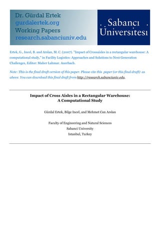
  • 3. 1. Introduction Order picking is generally the most significant operation in a warehouse, accounting for approximately 60% of all operational costs in a typical warehouse (Frazelle, 2001, page 147). Cost of order picking is affected by the decisions regarding the facility layout and the selection of storage and retrieval systems, and by the implemented strategies such as zoning, batching and routing. Travel cost is typically the largest cost component within order picking, accounting for about 50% of the costs associated with order picking activities (Frazelle and Apple, 1996). Since order picking, specifically traveling, is costly, reducing the travel time spent for order picking can significantly reduce operational costs. Figure 1. Case 0: A rectangular warehouse with four storage blocks, five main aisles, and no cross aisles (The vectors show a route to pick an order with seven items). In this chapter, we present the findings of a study that focuses on the strategic layout decisions of how many cross aisles to establish within a rectangular warehouse and how to determine the distances among them. A rectangular warehouse can be 2
  • 4. defined as a warehouse with equi-length parallel storage blocks, separated by aisles in between (Figure 1). A sub-region of a large warehouse where routing decisions are made independently from the remaining regions can also be considered as a rectangular warehouse, given that it satisfies the structural properties described above. A rectangular warehouse may have only main aisles which separate the storage blocks vertically (Figure 1), or may also contain one or more cross aisles perpendicular to the main aisles, which divide the storage blocks horizontally (Figures 2, 3 and 4). The main advantage of cross aisles is that they enable savings in travel times, especially during the order picking operations. Figures 1 and 2 illustrate an example of a rectangular warehouse where the creation of a cross aisle can reduce the travel distance while picking an order with seven items: The addition of the cross aisle (Figure 2) shortens the travel distance by enabling shortcuts from the 5th main aisle to the 4 th main aisle and from the 4th main aisle to the 3rd main aisle. Figure 2. The warehouse displayed in Case 0 with an interior cross aisle with shortcuts linking main aisle 5 to main aisle 4 and main aisle 4 to main aisle 3. 3
  • 5. Storage blocks typically consist of steel racks that are installed on the warehouse floor permanently during the construction of a warehouse. Thus the decisions regarding the quantities and dimensions of storage blocks, main aisles and cross aisles are strategic decisions. These decisions should be made considering many factors, including:  The physical dimensions of the building.  The characteristics of the materials to be stored, including physical dimensions, weights, shelf lives, pallet sizes and projected demand patterns.  The characteristics of warehouse equipment such as forklifts and AGVs.  The quantity and capabilities of the workforce.  The capabilities of the information system; i.e., the Warehouse Management System (WMS). One classic challenge raised by these factors is how to incorporate the interactions between different decision levels in the design and operation of warehouses (Rouwenhorst et al., 2000). For example, the strategic decision of determining the best warehouse layout, the tactical decision of assigning the products to the storage locations in the best way, and the operational decision of determining the best order picking routes are all interdependent. In our study we assume that the widths of the storage blocks, the main aisles and the cross aisles are fixed, and that the items stored in the warehouse all have the same demand frequencies. Even under these simplifying assumptions, the strategic decisions regarding the number of cross aisles and the distances between them (the lengths of storage blocks) have to be made by estimating the average travel distance in order picking under a specific routing algorithm. Hence, in our study we assume that 4
  • 6. the routing algorithm and the storage locations of products are pre-determined, and focus on the strategic decisions regarding cross aisles. Figure 3. A rectangular warehouse with equally spaced cross aisles (Case 1). Figure 4. A rectangular warehouse with unequally spaced cross aisles (Case 2). 5
  • 7. For a rectangular warehouse, one can identify the following three cases with respect to the number of cross aisles N and the distances in between them:  Case 0: Warehouse with no cross aisles (N=0), as shown in Figure 1.  Case 1: Warehouse with N equally spaced cross aisles (N1), as shown in Figure 3.  Case 2: Warehouse with N unequally spaced cross aisles (N1), as shown in Figure 4. In our study we seek answers to the following research questions regarding the rectangular warehouse: 1. Should the cross aisles be established equally spaced (Case 1) or unequally spaced (Case 2)? In other words, should the storage blocks have an equal length or variable lengths? 2. How much travel time savings do cross aisles bring? Under which settings do cross aisles bring the most travel time savings? 3. How many cross aisles should there ideally be in a rectangular warehouse? In other words, what is the best number of cross aisles? To answer these questions, we carry out extensive computational experiments reflecting a variety of warehouse settings with different values for warehouse lengths (T), number of cross aisles (M), and pick densities (D). Based on a thorough analysis of our experimental results, we come up with solid answers to the research questions posed above. One unique aspect of our research is that we extensively apply the starfield visualization technique from the field of information visualization. In starfield 6
  • 8. visualization, various fields of a dataset are mapped to the axes of a colored 2-D or 3-D scatter plot, and to the attributes of the glyphs (data points) such as color, size, and shape. Information visualization is the growing field of computer science that combines the fields of data mining, computer graphics, and exploratory data analysis (in statistics) in pursuit of visually understanding data (Keim 2002, Spence 2001). The ultimate goal in information visualization is to discover hidden patterns and gain actionable insights through a variety of -possibly interactive- visualizations. The use of a visualization approach in the analysis of our numerical results will enable us to make important observations, and develop managerial insights. To the best of our knowledge, this is the first attempt where data/information visualization techniques are employed to this extent in the warehousing and facility logistics literature. 2. Related Literature Rouwenhorst et al. (2000) present a reference framework and classification of warehouse design and operating problems. Van den Berg and Zijm (1999) provide another review of the warehousing literature that classifies warehouse management problems. Sharp (2000) summarizes functional warehouse operations, database considerations, and tactical, strategic and operational issues in warehouse planning and design. Within the vast facility logistics literature, there exists studies that solely focus on order picking routing and order batching for the purpose of reducing travel time. An early study by Ratliff and Rosenthal (1983) solves for the routing problem in order picking. Based on the number of aisles, the authors propose an algorithm that solves the problem 7
  • 9. to optimality. They state that the algorithm computation time grows linearly in the number of aisles, and is thus scalable for solving real world problems. Roodbergen and De Koster (2001) analyze the relationship between warehouse layout and average travel time. They consider a rectangular warehouse in which a single cross aisle divides the warehouse into two equal length blocks. The authors present a dynamic programming algorithm to determine the shortest order picking routes, and show that the addition of the cross aisle decreases average order picking time significantly. In another study, Roodbergen and De Koster (2001) compare several algorithms for routing order pickers in a warehouse with more than one cross aisle. They introduce two new heuristics, combined and combined+, and compare them with the S-Shape, Largest Gap and Aisle-by-Aisle heuristics in the literature. The authors prove through computational tests that the combined+ heuristic performs best among the five heuristics. A branch-and-bound algorithm is used as a benchmark to compare the performances of the generated heuristics. De Koster et al. (1999) report a real world application, where they significantly improve the efficiency of manual order picking activities at a large retail distribution center in Netherlands. In the first stage of their study, the authors apply a routing heuristic, which ensures that order pickers pick items from both sides of an aisle. This heuristic alone achieves a 30% reduction in travel time, and consequently a saving of 1.2 order pickers. In the latter stage of their study the authors apply order batching, time- savings method and a combined routing heuristic (De Koster and Van der Poort 1998) jointly, and achieve 68% reduction in travel distance and a saving of 3 to 4 pickers. This 8
  • 10. study is the perfect example of how the order picking strategies and routing algorithms proposed in the literature can be applied in the real world to achieve substantial savings. Our study is mainly related to the work of Vaughan and Petersen (1999), who consider both layout and routing. Vaughan and Petersen are motivated by the fact that cross aisles can reduce travel distances due to their flexibility in order picking. The authors develop a shortest path pick sequencing model that is applicable to any number of equally spaced cross aisles (equal length storage blocks) in the warehouse. Their model assumes that all the items along an aisle are picked before proceeding to the next aisle, and the order picking progresses from the leftmost aisle to the rightmost aisle. This policy is referred to as aisle-by-aisle policy. The authors compute the optimal routes for a large number of randomly generated picking requests, over a variety of warehouse layout and order picking parameters. Their results suggest that when the main storage aisle length (T) is small, an excessive number of cross aisles can increase the average travel distance. This is true especially when the number of storage aisles (M) is small, and when pick density is very small or very large. The authors warn that the savings due to cross aisles diminish, even turn into losses, if the number of cross aisles becomes excessive. This is because the extra distance to traverse the cross aisles increases the travel distances. Additionally, the authors find out that as the main storage aisle length (T) increases the optimal number of cross aisles also increases and report that cross aisles are most beneficial for longer warehouses. 9
  • 11. 3. The Vaughan and Petersen Model Vaughan and Petersen (1999) assume certain characteristics with respect to the rectangular warehouses and order picking policies. Since our study is built on their model, which we will refer to as the V&P model, these assumptions are also valid for our model:  There are parallel main aisles and products are stored on both sides of the main aisles.  Each order includes a number of items to be picked, which are generally located in various main aisles.  All stocks of a particular item are stored in a single location.  Order pickers can traverse the aisles in both directions and change directions within the main aisles.  The main aisles are narrow enough to pick from both sides of the aisle without changing position.  The main aisles are wide enough such that two or more order pickers can operate in the main aisle at the same time.  There are two natural cross aisles in the warehouse, at the head and rear of the warehouse.  Cross aisles are not used to store items; they are only used to pass to the next main aisle.  The items of an order are collected in a single tour. Block lengths are determined by the locations of the cross aisles that divide main aisles perpendicularly. In our study, the number of cross aisles refers to the number of 10
  • 12. interior cross aisles, which are between the default head and rear cross aisles. We assume that picking routes start and end at the southeast and southwest corners of the warehouse, respectively. Even though some research assumes that order picking ends at the starting point (De Koster and Van der Poort 1998, Roodbergen and De Koster 2001), this does not make a great change in travel distance (and thus travel time). Petersen (1997) notes that this change results in at most 1% deviation in travel distance. (a) (b) Figure 5. (a) A warehouse with storage blocks of equal lengths and (b) a warehouse with storage blocks with unequal lengths (Arrows represent the total vertical travel distance to pick items in main aisle m when the main aisle is entered from the ith cross aisle and left from the jth cross aisle). The dynamic programming algorithm developed by Vaughan and Petersen (1999) finds the optimal route to pick an order under the aisle-by-aisle policy. The complete notation for their so called shortest path model is as follows: L: Length of a storage block. T: Length of the warehouse (equal to the length of main aisles), T   N  1L . 11
  • 13. M: Number of main aisles. N: Number of interior cross aisles (The total number of cross aisles is N+2). A: Width of a cross aisle. This parameter is essential for the calculation of the best aisle- by-aisle route. The model assumes that an order picker walks along the center of the cross aisles. This walking pattern is illustrated in Figure 5 and the additional distance of A/2 to walk to the middle of the cross aisle is reflected in the formulas for B1m and B2 m. B: Width of a main aisle. C: Width of a storage block. The notation until now is related to the warehouse layout. The notation below is given for to a particular order to be picked: Km: The number of items to be picked by the order picker from main aisle m = 1, 2, .., M. M Thus the order consists of K m 1 m items in total. Xm(t): The location of an item t in main aisle m = 1, 2, …, M, and t = 1, 2, …, K m (undefined if Km = 0) where 0  Xm(t)  T. (The expressions listed below are demonstrated in Figure 5a.) Xm+: The location of the item at the south-most location (highest value) in main aisle m (undefined if Km = 0), i.e. Xm+ = max  X m (t ) . t Xm-: The location of the item at the north-most location (smallest value) in main aisle m (undefined if Km = 0), i.e. Xm- = min  X m (t ) . t Cm(i,j): The total vertical travel distance required to pick all the items in main aisle m, if main aisle m is entered at cross aisle i and exited to main aisle m-1 at cross aisle j. 12
  • 14. B1m(i,j): The length of forward-tracking leg required to pick the items in main aisle m to the north of cross aisle h, h = min (i,j). B2m(i,j): The length of back-tracking leg required to pick the items in main aisle m to the south of cross aisle h, h = max (i,j). fm(i): The minimum total picking distance required to pick all the items in aisle m, m-1, m-2, ..., 2, 1 if main aisle m is entered at cross aisle position i. In the V&P model Cm, B1m, and B2m are calculated as follows: C m (i , j )  B1m (i, j )  i  j ( L  A)  B 2 m (i , j ) ; where  0 for K m  0,   B1m (i , j )   0 for X  min(iL, jL), m   2 min(iL, jL)  X   A(0.5  ((min(iL, jL)  X  ) / L)) m m  for  X  min(iL, jL); m and  0 for K m  0,   B 2 m (i , j )   0 for X  max(iL, jL ), m  2 max(iL, jL )  X  A(0.5  (( X   max(iL , jL )) / L))   m m  for  X  max(iL, jL ). m The dynamic programming equations for each stage are given as follows: fm (i)  min Cm (i, j )  f m1 ( j ) , where f1 (i )  C1 (i , N  1) . j Stages of the dynamic programming are related to the main aisle numbers in the warehouse. The desired shortest-path picking route is determined by evaluating f M ( N  1) . 4. The Modified Model Now we present our model that allows us to find the best routes according to the aisle-by- aisle heuristic for the case of unequally-spaced cross aisles (Case 2). The primary 13
  • 15. difference between our model and the V&P model is that the storage blocks now have variable lengths Li (Figure 5b) instead of a fixed length of L (Figure 5a) where Li is the length of the ith storage block for i = 1,…, N+1. Thus, the length of the warehouse T N 1 which is equal to the length of the main aisles can be expressed as T   Li . i 1 Next, we define two new notations that give us the indices of the blocks where the north- most and south-most items within an aisle are located: Blockof(Xm+): Index of storage block Li in main aisle m where Xm+ is located for i = 1, 2, …, N+1. Blockof(Xm-): Index of storage block Li in main aisle m where Xm- is located for i = 1, 2, …, N+1. Finally, the Cm, B1m and B2m values are calculated based on the modified definitions of block lengths Li and the warehouse length T which can be expressed as: max( i , j ) Cm (i, j )  B1m (i , j )   s  min( i , j ) 1 Ls  i  j A  B 2m (i , j ) , where  i j  B1m (i, j )  2  min( Ls ,  L f )  X   A(0.5  min(i, j )  Blockof ( X  ))  , and m m   s 1 f 1    i j  B 2m (i , j )  2  X   max( Ls ,  L f )  A(0.5  Blockof ( X  )  1  max(i, j ))  m m   s 1 f 1   5. Algorithms to Identify Best Storage Block Lengths Li Given T, M, N, A, B, C and D values, the problem of finding the best storage block lengths Li is a difficult problem. This is because the length of a tour is found by 14
  • 16. solving a dynamic programming problem and the locations of the items are uniformly distributed. The objective function to be minimized is the average travel distance (and thus, the average travel time) over all orders, with the optimal travel distance for each order computed through dynamic programming optimization. We thus develop and implement two heuristic search algorithms, namely GSA (Grid Search Algorithm) and RGSA (Refined Grid Search Algorithm), to find the best Li values. GSA takes a warehouse (with its T, M, N, A, B, C values), a set of generated orders and the number of grids as parameters, and identifies an initial solution, which consists of Li values. RGSA takes the solution of GSA as the initial solution and carries out a search to reduce the average travel distance (i.e., average travel time). These algorithms are given in pseudo- code and are explained in the Appendix. Table 1. Experimental design. Factor Number of values Values Length of main aisles (T) (meters) 6 30, 60, 90, 120, 150, 180 396 scenarios Number of main aisles (M) 6 5, 10, 15, 20, 25, 30 Pick density (D) 11 0.1, 0.5, 1.0, 1.5, 2.0, (items/aisle) 2.5, 3.0, 3.5, 4.0, 4.5, 5.0 Number of cross aisles (N) 1 (for Case 0) 0 8 (for Case 1) 1, 2, 3, 4, 5, 6, 7, 8 3 (for Case 2) 1, 2, 3 (A, B, C) * (meters) 1 (2.50, 1.25, 1.25) *: A: Width of a cross aisle; B: Width of a main aisle; C: Width of a storage block 15
  • 17. 6. Experimental Design The different values of model parameters that we have used in our computational experiments are depicted in Table 1. We investigate 396 scenarios (problem instances) corresponding to 396 combinations of the warehouse length (T), the number of aisles (M) and the pick density (D). In all these scenarios, the A, B, C parameters are respectively set to fixed values of 2.50, 1.25 and 1.25 (meters). Figure 6. Savings with respect to the pick density (D). One fundamental parameter is the pick density (D), which is the average number of items per main aisle. In each scenario, the total number of items to be picked is calculated as the multiplication of the pick density (D) with the number of main aisles (M). The 11 pick density values listed above are used for calculating the order sizes during the estimation of average route length for each scenario. Thus the 11 order sizes 16
  • 18. used in the experiments are 0.1M, 0.5M, 1.0M, 1.5M, 2.0M, 2.5M, 3.0M, 3.5M, 4.0M, 4.5M and 5.0M. Figure 7. Savings with respect to the warehouse length (T). The parameter values in our study are selected such that we can extend the experiments of Vaughan and Petersen (1999). Compared to the 126 scenarios (combinations of T, M and D) in their study, we consider 396 scenarios. In addition, our parameters take values over broader ranges, we calculate average travel distances over a greater number of instances (1000 orders as opposed to 100 instances), and we consider Case 2 besides Case 1. For each warehouse (T, M, N, A, B, C) and for each order size (D*M) we apply the following procedure: Step 1: Generate a set of 1000 orders with D*M items each: Each item to be picked is assigned to a storage location by first randomly generating a main aisle number, and then, 17
  • 19. randomly generating the position within that main aisle on the interval [0, T). The locations of the items to be picked in each order are assumed to be uniformly distributed across the warehouse. This assumption can be encountered in related studies (e.g.; see Roodbergen and De Koster, 2001). Step 2: Apply RGSA. Step 2.a: Apply GSA for the generated set of orders and the given warehouse: For each feasible configuration of storage blocks, the shortest path dynamic programming algorithm of the V&P model is solved for each of the orders in the set of orders. Average travel distances in the set of orders is obtained and an initial best configuration of storage blocks that provides the minimum average order picking travel distances is returned. Step 2.b: Apply the remaining steps of RGSA: Given the initial solution returned by GSA, RGSA works on improving the Li values with the objective of minimizing average travel distance. In Step 1 of the above procedure, the seed used to generate the random numbers is always chosen the same. The result of the experiments is a dataset with 396 rows and the following 17 columns: T, M, N, D, average travel length in Case 0, average travel length in Case 1 for N=1, 2, …, 8 (8 distinct columns), average travel length in Case 2 for N=1, 2, 3 (3 distinct columns), area of the warehouse (for the scenario). We carry out our analysis in Section 7 using this dataset. The values in the dataset are computed through a heuristic algorithm (which is not optimal) and through Monte Carlo simulation. Since we 18
  • 20. are using heuristic algorithms, from now on, the solution which will be referred to as the best solution is actually the incumbent solution, which is not necessarily optimal. Figure 8. Savings with respect to the number of main aisles (M). 7. Analysis of Experimental Results In this section we analyze, through starfield visualizations, the results of our computational experiments for the 396 scenarios. The first three figures that we discuss in this section (figures 6, 7and 8) are referred to as colored scatter plots in exploratory data analysis literature (Hoffman and Grinstein, 2002). According to this naming scheme, Figures 9 and 10 are referred to as jittered colored scatter plots, and figures 11, 12, and 13 are referred to as colored 3-D scatter plots. However, rather than using the terminology in exploratory data analysis, we refer to all these plots as starfield visualizations, following the terminology in the field of information visualization 19
  • 21. (Shneiderman, 1999). The starfield visualization is an extended version of the scatter plot, with coloring, size, zooming and filtering. Figure 9. Percentage travel time savings with respect to the warehouse length (T) and number of main aisles (M). In each of figures 6 through 13, information regarding which parameter is mapped to which attribute of the plot/glyphs is displayed below the plot. For example, in Figure 6, D (pick density) values are mapped to color of the glyphs, percentage travel time savings (in Case 2 compared to Case 1) are mapped to the X-axis, and percentage space savings (in Case 2 compared to Case 1) are mapped to the Y-axis. The range of pick density values is 0 to 5. Lighter colors represent larger values of the mapped parameter, and darker colors represent smaller values of the mapped parameter. All the mappings are linear. Rectangular frames, such as frames (a) and (b) in Figure 6, are drawn to highlight specific regions in the plots that exhibit the interesting properties. 20
  • 22. Figure 10. Percentage Space savings with respect to the warehouse length (T) and number of main aisles (M). 7.1. Savings in Case 2 Compared to Case 1 Figures 6 through 10 illustrate the percentage savings gained in layouts with unequally spaced cross aisles (Case 2) compared to layouts with equally spaced cross aisles (Case 1). In figures 6, 7 and 8, each scenario is represented by a glyph (data point), the percentage travel time (distance) savings in Case 2 compared to Case 1 are mapped to the X-axis, the percentage space savings are mapped to the Y-axis, and various parameters (D, T, and M) are mapped to colors of the glyphs. In Figures 9 and 10, each scenario is again represented by a glyph, but this time the T values are mapped to the X- axis, the M values are mapped to the Y-axis, and the percentage savings (in travel time and in warehouse space) are mapped to colors of the glyphs. 21
  • 23. In Figure 6, frame (a) shows that the scenarios with large percentage travel time savings are all characterized by high pick densities (large D values). Frame (b) shows that under certain scenarios, the percentage travel time savings are obtained only at the cost of big losses in warehouse space (negative percentage space saving values on the Y-axis). In Figure 7, frame (a) shows that the scenarios with the largest percentage travel time savings are for warehouses that have medium T values. Frames (b) and (c) show that scenarios which benefit from Case 2 with respect to percentage space savings are all characterized by large length values (light colors). However, in these scenarios there may be savings as well as losses in percentage travel time, as can be seen in Frames (a) and (b), respectively. Frame (d), on the other hand, shows that in instances with shorter warehouses (glyphs with darker colors) the best number of cross aisles for Case 2 is more than the best number of cross aisles for Case 1, and this can result in large percentage losses in warehouse space. These instances are all characterized by high pick densities in from frame (b) of Figure 6. In Figure 8, the frame shows that the scenarios in which Case 2 results in significant space savings, but also the travel time losses (negative values on the X-axis) are all characterized by large M values (light tones of gray). From figures 6 and 7, we remember that these are also scenarios with low pick densities and largest T values. The maximum percentage travel time saving (X value of the rightmost glyph) obtained in the 396 scenarios is 5.28%. This result strikingly suggests that unequally spaced cross aisles (Case 2) bring little additional savings in comparison to equally spaced cross aisles (Case 1). In our study, finding the best number and best positions of unequally spaced cross aisles required implementation of a non-trivial algorithm and 22
  • 24. allocation of significant running times for the computations (approximately ten days in total, most of it for computing the solutions for N=3 in Case 2). Thus, we can conclude that warehouse planners are better off establishing rectangular warehouses with equally- spaced cross-aisles instead of unequally-spaced cross-aisles. These results provide answers to the first research question posed in Section 1. Figure 11. Percentage Travel time savings with respect to the warehouse length (T), number of main aisles (M) and pick density (D) for N=1. Figures 9 and 10 allow the analysis of savings with respect to T and M, which are mapped to the X and Y-axes, respectively. Since there are 11 scenarios for each (T, M) pair, jittering is applied to a certain extent to avoid occlusion. So in these two figures the glyphs which are clustered together have the same T and M values, but differ in their pick densities (D values). 23
  • 25. In Figure 9, frame (a) shows that for small values of T, percentage travel time savings in Case 2 are higher in general (lighter glyphs). For large warehouses, which are highlighted by frame (b), there are less savings, or even losses in Case 2. This may be due to the fact that our algorithm finds the best positions in Case 2 is run only for N=1, 2, and 3. We thus believe that development of efficient algorithms for solving Case 2 for larger values of N is critical. Figure 12. Percentage travel time savings with respect to the warehouse length (T), number of main aisles (M) and pick density (D) for N=5. In Figure 10, frame (a) shows that shorter warehouses can incur big space losses in Case 2, since for the associated scenarios, the best number of cross aisles required in Case 2 (to minimize travel time) is typically more than the number of cross aisles required in Case 1. Frame (b) shows, as expected, that there are space savings in Case 2 compared to Case 1, since N3 in Case 2 and N8 in Case 1. In general, through 24
  • 26. our observations in Section 7.1, we can conclude that it is sufficient to focus only on Case 1 which we continue to analyze in Sections 7.2 and 7.3. 7.2. Impact of T, M and D in Case 1 Figures 11 and 12 show the change in percentage travel time savings in Case 1 (for N=1 and N=5) compared to Case 0, under the 396 combinations of T, M and D (which are mapped to X, Y, and Z axes, respectively). Percentage travel time saving in each scenario is mapped to color of the related glyph. As shown in frame (a) of both figures, the largest travel time savings are realized for pick densities (D values) between 0.5 and 2.5. This observation is consistent with earlier findings of Vaughan and Petersen (1999), who state that “the greatest cross aisle benefit occurs at pick densities in the range 0.6 to 1.0 units/aisle,” which answers the second research question posed in Section 1. 25
  • 27. Figure 13. The best number of cross aisles (N) with respect to the warehouse length (T), number of main aisles (M) and pick density (D). In both figures 11 and 12, the impact of M is observed to be negligible, except for D=0.1 (warehouses with very small orders). This conclusion is reached by observing that the colors of the glyphs do not change significantly along the Y-axis, except for D=0.1. Meanwhile, as shown in frame (b) of both figures, shorter warehouses (with small T values) are most sensitive to changes in D. Vaughan and Petersen (1999) also state that the “addition of cross aisles generally decreases the picking travel distance on average, with travel distances frequently in the range 70%-80%, or even less, of that associated with the no cross aisles N=0 layout,” quantifying the savings that can be obtained. This is another significant finding of our study. The percentage travel time savings in figures 11 and 12 take values between 0 and 35.30. That is, we observe travel time savings of up to 35.30% by adding cross aisles, confirming the earlier findings of the authors. Table 2. The best number of cross aisles for different (T, M) pairs, accompanied with the maximum travel time losses that one can encounter under any D. T=30 T=60 T=90 T=120 T=150 T=180 M=5 1 2 2 3 4 4 0.52% 1.32% 0.51% 0.30% 0.59% 0.37% M=10 1 2 3 3 4 4 1.86% 0.32% 0.23% 0.66% 0.58% 0.38% M=15 1 2 3 4 4 5 2.40% 0.86% 0.22% 0.10% 0.35% 0.21% M=20 2 3 3 4 4 5 2.55% 0.81% 0.44% 0.10% 0.31% 0.10% 26
  • 28. M=25 2 3 3 4 5 5 2.43% 0.74% 0.42% 0.18% 0.31% 0.12% M=30 2 3 3 4 5 5 2.45% 0.74% 0.54% 0.16% 0.27% 0.15% 7.3. Best Number of Cross Aisles in Case 1 Figure 13 shows the change in the best number of cross aisles in Case 1, which is mapped to color. The parameters T, M, and D are again mapped to X, Y, and Z axes, respectively. Since none of the scenarios has its best N value equal to 8, the range of N values is between 1 and 7. Also, since the glyphs in the figure do not have the lightest tones of gray, we can observe that the best N values are seldom 7 or 6. A count in the experimental results shows that in 389 (all but 7) of the 396 scenarios, the best N value is less than or equal to 5. The most frequently encountered N value is 4, with 129 scenarios implying that N=4 is the most desirable number of cross aisles. We can conclude from Figure 13 that the main determinant of the best N value is the warehouse length T, since there are big changes in the color tone as one goes from smaller to larger values of T. By judging from the pattern of change in color tone, one can conclude that M also has some impact as well. At this point, we can address the third research question stated in Section 1 in two parts, both of which are very relevant and important: What is the best number of cross aisles for known values of T and M? And is there a best number of cross aisles, regardless of T and M? The first question is very relevant, since in designing warehouse layouts, warehouse planners typically have a very limited knowledge on future D values, while they generally have a good judgment of which values T and M should take. The answer to the first question is given in Table 2, which displays the best number of cross aisles for 27
  • 29. different (T, M) pairs, accompanied with the maximum travel time losses that one can encounter under any D values. For example, for (T, M)=(90, 10), the planner should establish 3 cross aisles. Among the 11 D values tested in our experiments for this (T, M) combination, establishing a different number of cross aisles resulted in at most 0.23% savings compared to 3 cross aisles. Figure 14. The maximum percentage gap –over all scenarios– between the travel time under N and the best travel time for that scenario. The second question is very relevant as well, since many warehouse planners would prefer to learn and always remember a single number, rather than having to refer to Table 2 in this chapter. Thus, the question is which number of cross aisles to recommend to a warehouse planner regardless of T, M, or D values. The answer to this question is simply 3. A warehouse planner can always build warehouses with 3 equally spaced cross aisles without compromising a significant loss in travel time, in particular, when compared to warehouses with different numbers of cross aisles. 28
  • 30. Of course, this result is valid if the A, B, C values are close to the values in Table 1, and the warehouse operates under the assumptions of our model, including the usage of the aisle-by-aisle policy for routing. For the scenarios that we analyze in our experiments, the worst travel time loss for 3 cross aisles is 6.26% (Figure 14), and the worst warehouse space (area) loss is 15.38% (Figure 15). Figures 14 and 15 show the worst average losses for other values of N. Figure 15. The maximum percentage gap –over all scenarios– between the warehouse space under N and the warehouse space for the best N for that scenario. If the warehouse space (area) is the most critical resource, then a warehouse planner can establish 2 cross aisles, instead of 3. In our experiments, having 2 cross aisles resulted in at most 16.68% loss in travel time (Figure 14), and 7.69% loss in warehouse space (Figure 15). Thus, layouts with 3 (equally spaced) cross aisles are robust in terms of travel time, and layouts with 2 cross aisles are robust in terms of warehouse space. 29
  • 31. 8. Conclusions and Future Work In this chapter, we presented a detailed discussion of the impact of cross aisles on a rectangular warehouse. We analyzed both equally spaced and unequally spaced cross aisles, which we referred to as Case 1 and Case 2, respectively. For Case 1 we utilized the dynamic programming algorithm presented in Vaughan and Petersen (1999) to determine the optimal order picking routes under aisle-by-aisle policy. For Case 2, we made modifications to the Vaughan and Petersen (1999) model, including the change of formulas for certain parameters and introduction of new expressions before running the dynamic programming algorithm. We computed the average travel times using Monte Carlo simulation for 396 distinct scenarios, which correspond to 396 different warehouse and demand combinations. Our primary findings are: 1. It is more desirable to establish only equally-spaced cross aisles than to establish unequally spaced cross aisles. 2. Establishing (equally spaced) cross aisles can bring significant travel time savings and should definitely be considered: We obtained savings up to 35.30% in our experiments. Biggest travel time savings are realized for pick densities between 0.5 and 2.5 (D[0.5, 2.5]). 3. Given the length of main aisles and the number of main aisles (T and M), warehouse planners can refer to Table 2 in this chapter to determine the best number of (equally spaced) cross aisles. If one does not wish to refer to this table, but wishes to learn and remember a single value for the best number of cross aisles, we propose the value of 3. 30
  • 32. There are several directions for future research relating to our study. Below we list two: 1. It is necessary to design faster and better algorithms to identify the best storage block lengths (Li) in Case 2, and to validate further our first conclusion. 2. It is important to test the robustness of our conclusions under other demand patterns and different routing heuristics. Our study contributes to the research and practice of warehouse planning / facility logistics by providing actionable insights regarding cross aisles. There is a great potential for research that attempts to solve warehousing problems that require taking interdependent decisions at different time horizons; for example at both strategic and operational levels. Finally, we suggest the adoption of data analysis techniques from the field of information visualization for discovering knowledge hidden in experimental and empirical data related to warehouse planning. Acknowledgements The authors thank Kemal Kılıç at Sabancı University for his extensive help in reviewing the M.S. thesis of Bilge Incel (Küçük), which in time turned into this chapter. The authors also thank Ş. İlker Birbil for reviewing the final draft of the paper and suggesting many improvements. 31
  • 33. References De Koster, R., Roodbergen, K. J., Van Voorden, R. (1999) “Reduction of walking time in the distribution center of De Bijenkorf,” in New Trends in Distribution Logistics, M. Grazia Speranza, Paul Stähly, Eds., Springer-Verlag Berlin Heidelberg. De Koster, R., Van der Poort, E. (1998) “Routing order pickers in a warehouse: a comparison between optimal and heuristic solutions,” IIE Transactions, vol: 30, pp. 469-480. Hoffman, P. E., Grinstein, G. G. (2002) “A survey of visualiations for high-dimensional data mining,” in Information Visualization in Data Mining and Knowledge Discovery, Usama Fayyad, Georges Grinstein and Andreas Wierse, Eds., Morgan Kaufmann. Frazelle, E. H. (2001) World-class warehousing and material handling. McGraw-Hill. Frazelle, E. H., Apple, J. M. (1994) “Warehouse operations,” in The Distribution Management Handbook. James A. Tompkins and Dale Harmelink, Eds. Mc- Graw-Hill. Keim, D. A. (2002) “Information visualization and visual data mining,” IEEE Transactions on Visualization and Computer Graphics, vol: 8 no: 1, pp.1–8 Petersen, C.G. (1997) “An evaluation of order picking routing policies,” International Journal of Operations and Production Management, vol: 17, pp. 1098-1111. Ratliff, H. D., Rosenthal, A. S. (1983) “Order Picking in a rectangular warehouse: A solvable case of the traveling salesman problem,” Operations Research, vol: 31, no: 3, pp. 507-521. 32
  • 34. Roodbergen, K. J., De Koster, R. (2001a) “Routing order pickers in a warehouse with a middle aisle,” European Journal Of Operational Research, vol: 133, pp. 32-33. Roodbergen, K. J., De Koster, R. (2001b) “Routing methods for warehouses with multiple cross aisles,” International Journal of Production Research, vol: 39, pp. 1865-1883. Rouwenhorst, B., Reuter B., Stockrahm, V., Van Houtum, G. J., Mantel, R. J., Zijm, W. H. M. (2000) “Warehouse design and control: framework and literature review,” European Journal of Operational Research, vol: 122, pp. 515-533. Sharp, P.G. (2000) “Warehouse management,” Chapter 81 in Handbook of Industrial Engineering, Gavriel Salvendy, Ed., John Wiley & Sons, Inc., New York. Shneiderman, B. (1999) “Dynamic queries, starfield displays, and the path to Spotfire”. Available under http://www.cs.umd.edu/hcil/spotfire/ . Retrieved on November 2006. Spence, R. (2001) Information visualization. Essex, England: ACM Press. Van den Berg, J. P., Zijm, W. H. M. (1999) “Models for warehouse management: classification and examples,” International Journal of Production Economics, vol: 59, pp. 519-528. Vaughan, T. S., Petersen, C. G. (1999) “The effect of warehouse cross aisles on order picking efficiency,” International Journal of Production Research, vol: 37, pp. 881-897. 33
  • 35. Appendix GRID_SEARCH_ALGORITHM (GSA) This algorithm returns bestL, the best block lengths among tested layouts, for a given N. The length of the gridForL array is (N+1) and indicates the number of storage blocks. gridsForL[i] records the number of grids that constitute the length of the ith storage block. If the summation of the elements of gridForL array is equal to noOfGrids value, then a feasible storage block length combination is obtained. When noOfGrids = 20 and N = 2, for example, then some of the feasible storage block lengths (L1, L2, L3) would be (1, 12, 7), (11, 4, 5), having the summation of L values equal to noOfGrids = 20. GSA generates feasible configurations of storage blocks systematically and returns the travel distances by solving the modified model that we present for a uniformly distributed set of orders. Average of the travel distances for the order set is taken and the initial best configuration of storage blocks enabling the minimum average order picking travel distances is labeled as bestL. This algorithm generates a greater number of feasible storage block length alternatives as the number of grids is increased. This results in smaller unit length (G= T/noOfGrids). However, the more the number of feasible solution gets, the more will be the computational effort. We observed in our experiments that for the warehouse and order settings described in the next section, noOfGrids = 7 is computationally prohibitive (18 days running time including the cases where N = 4), and noOfGrids is selected as seven. 34
  • 36.  = {1,...., N+1}, O = {1,...., } GRID_SEARCH_ALGORITHM (warehouse, orders, noOfGrids) G = T/noOfGrids ........... for each gridsForL, /* s.t. gridsForL[i]  noOfGrids, i */ sumOfGrids =  i gridsForL[i] if( sumOfGrids = = noOfGrids&&ARRAY_CONTAINS_NOZERO(gridsForL)) tempL[i] = gridsForL[i] * G, i   TempWarehouse.setL(tempL) orders[o].setWarehouse(tempWarehouse), o  O tempSimulationStatistics = CALCULATE_SIMULATION_STATISTICS(orders) tempTravelDistance = tempSimulationStatistics.getAverage() if (tempTravelDistance < bestTravelDistance) bestL = tempL bestTravelDistance = tempTravelDistance return bestL CALCULATE_SIMULATION_STATISTICS (orders) travelDistance[o] = getOptimalTravelDistance( orders[o] ), o  O return statistics for travelDistance data 35
  • 37. REFINED_GRID_SEARCH_ALGORITHM (RGSA) This algorithm starts with the result of the grid search algorithm as the initial solution and applies changes in little unit lengths (G) to the initial best configuration of storage blocks (initialBestL). In this method, first a range is defined. Half of this range is subtracted from each storage space length and smaller unit lengths (gridsForL[i]*G) are added to each storage space length. The travel distance for the new configuration tempL is calculated for the given order set (orders) and compared with the best result obtained until that time. After trying all feasible configurations of the gridsForL for the same initial solution and calculating the travel distance for the new storage block lengths, tempL resulting in the shortest travel distance is assigned as the best configuration of cross aisles, bestL. Then the range is updated by dividing with the number of grids (noOfGrids). Half of this range is subtracted from each storage space length and smaller unit lengths (gridsForL[i]*G) are added to obtain new feasible storage block lengths (tempL) and travel distance implied by the updated tempL is calculated for the given order set (orders). The refined grid search is continued until the range declines to a length, which is determined as the smallest range (resolution) to be considered. When the range becomes as small as the resolution, the refined grid search is terminated and the improved configuration of storage block lengths is assigned as the best configuration of storage block lengths (bestL) for the given warehouse and order set. Any element of gridsForL can be at most (N+1)*noOfGrids, because in the refined grid search algorithm for each storage block, half of the range is subtracted and the length gridsForL[i]*G is added, for instance: From the above equations it is clearly seen that summation of the gridsForL’s 36
  • 38. elements has to be (N+1)*noOfGrids. Therefore, an element of gridsForL is allowed to be (N+1)*noOfGrids at most. The search algorithms result in the best storage block lengths that give the minimum order picking travel distance for a problem instance (T, M, N, A, B, C, D) among the tested configurations. REFINED_GRID_SEARCH_ALGORITHM(warehouse, orders, noOfGrids, resolution) initialBestL = GRID_SEARCH_ALGORITHM(warehouse, orders, noOfGrids) range = T/noOfGrids iterationNo = 0 continueFlag = true while (continueFlag) iterationNo++ if (iterationNo > 1) // if not the first iteration range = (range/noOfGrids)/2 G = (range/noOfGrids)/2 for each gridsForL /* gridsForL[i]  (N+1)*noOfGrids */ sumOfGrids =  i gridsForL[i] if (sumOfGrids==(N+1)noOfGrids&&ARRAY_CONTAINS_NOZERO(gridsForL)) tempL[i] = initialBestL[i] – (range/2) + gridsForL[i]*G, i   tempWarehouse.setL(tempL) orders[o].setWarehouse(tempWaarehouse), o  O 37
  • 39. tempSimulationStatistics=CALCULATE_SIMULATION_STATISTICS(orders) tempTravelDistance = tempSimulationStatistics.getAverage() if (tempTravelDistance < bestTravelDistance) bestL = tempL bestTravelDistance = tempTravelDistance if(range<resolution) continueFlag = false return bestL 38