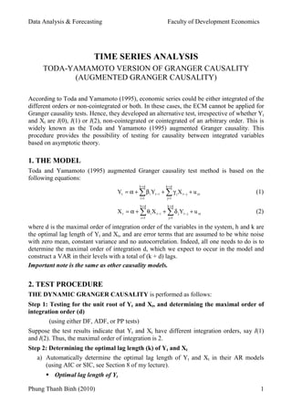
1. Data Analysis & Forecasting Faculty of Development Economics
TIME SERIES ANALYSIS
TODA-YAMAMOTO VERSION OF GRANGER CAUSALITY
(AUGMENTED GRANGER CAUSALITY)
According to Toda and Yamamoto (1995), economic series could be either integrated of the
different orders or non-cointegrated or both. In these cases, the ECM cannot be applied for
Granger causality tests. Hence, they developed an alternative test, irrespective of whether Yt
and Xt are I(0), I(1) or I(2), non-cointegrated or cointegrated of an arbitrary order. This is
widely known as the Toda and Yamamoto (1995) augmented Granger causality. This
procedure provides the possibility of testing for causality between integrated variables
based on asymptotic theory.
1. THE MODEL
Toda and Yamamoto (1995) augmented Granger causality test method is based on the
following equations:
h +d k +d
Yt = α + ∑ β i Yt −i + ∑ γ j X t − j + u yt (1)
i =1 j=1
h+d k +d
X t = α + ∑ θ i X t −i + ∑ δ j Yt − j + u xt (2)
i =1 j=1
where d is the maximal order of integration order of the variables in the system, h and k are
the optimal lag length of Yt and Xt, and are error terms that are assumed to be white noise
with zero mean, constant variance and no autocorrelation. Indeed, all one needs to do is to
determine the maximal order of integration d, which we expect to occur in the model and
construct a VAR in their levels with a total of (k + d) lags.
Important note is the same as other causality models.
2. TEST PROCEDURE
THE DYNAMIC GRANGER CAUSALITY is performed as follows:
Step 1: Testing for the unit root of Yt and Xt, and determining the maximal order of
integration order (d)
(using either DF, ADF, or PP tests)
Suppose the test results indicate that Yt and Xt have different integration orders, say I(1)
and I(2). Thus, the maximal order of integration is 2.
Step 2: Determining the optimal lag length (k) of Yt and Xt
a) Automatically determine the optimal lag length of Yt and Xt in their AR models
(using AIC or SIC, see Section 8 of my lecture).
Optimal lag length of Yt
Phung Thanh Binh (2010) 1

2. Data Analysis & Forecasting Faculty of Development Economics
h
Yt = α + ∑ β i Yt −i + u yt (3)
i =1
Restricted model
Estimate (4) by OLS, and obtain the RSS of this regression (which is the restricted
one) and label it as RSSRY.
h +d d
Yt = α + ∑ β i Yt −i + ∑ γ j X t − j + u yt (4)
i =1 j=1
Optimal lag length of Xt
h'
X t = α + ∑ θ i X t −i + u xt (5)
i =1
Restricted model
Estimate (6) by OLS, and obtain the RSS of this regression (which is the restricted
one) and label it as RSSRX.
h '+ d d
X t = α + ∑ θ i X t −i + ∑ δ j Yt − j + u xt (6)
i =1 j=1
b) Manually determine the optimal lag length of Xt (k in equation (1)) and Yt (k in
equation (2)), (using AIC or SIC, depending on which one you use in step 2a, see
Section 8 of my lecture).
h +d k +d
Yt = α + ∑ β i Yt −i + ∑ γ j X t − j + u yt (7)
i =1 j=1
Then estimate (7) by OLS, and obtain the RSS of this regression (which is the
unrestricted one) and label it as RSSUY.
h '+ d k '+ d
X t = α + ∑ θ i X t −i + ∑ δ j Yt − j + u xt (8)
i =1 j=1
Then estimate (8) by OLS, and obtain the RSS of this regression (which is the
unrestricted one) and label it as RSSUX.
Step 3: Set the null and alternative hypotheses
a) For equation (4) and (7), we set:
k
H0 : ∑γ
j=1
j = 0 or X t does not cause Yt
k
H1 : ∑γ
j=1
j ≠ 0 or X t causes Yt
b) For equation (6) and (8), we set:
k'
H0 : ∑δ
j=1
j = 0 or Yt does not cause X t
Phung Thanh Binh (2010) 2

3. Data Analysis & Forecasting Faculty of Development Economics
k'
H1 : ∑δ
j=1
j ≠ 0 or Yt causes X t
Step 4: Calculate the F statistic for the modified Wald test
a) For equation (4) and (7), we set:
(RSS RY − RSS UY ) / k
F=
RSS UY /( N − K )
where K is the number of estimated coefficients.
b) For equation (6) and (8), we set:
(RSS RX − RSS UX ) / k '
F=
RSS UX /( N − K )
where K is the number of estimated coefficients.
If the computed F value exceeds the critical F value, reject the null hypothesis and
conclude that Xt weakly causes Yt, or Yt weakly causes Xt.
Questions: How to explain the test results?
Phung Thanh Binh (2010) 3