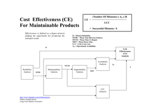
1. (Number Of Missions) x AO x R
Cost Effectiveness (CE) CE =
LCC
For Maintainable Products = Successful Missions / $
Effectiveness is defined as a figure-of-merit
judging the opportunity for producing the R = Mission Reliability
intended results MTBF = Mean Time Between Failures
MTTR = Mean Time To Repair
MDT = Mean Down Time
LCC = Life Cycle Cost
AO = Operational Availability
R
Cost
Effectiveness
(CS)
Analysis
Availability
Analysis AO
MTTR
$
Reliability Maintainability Supportability
MDT
Analysis MTBF Analysis Analysis
LCC
Analysis
http://www.linkedin.com/in/hilaireperera
Hilaire Ananda Perera
Long Term Quality Assurance

2. Parameters Related
To
Cost Effectiveness (CE)
Reliability (R)
β
T .Γ 1 1
MTBF β
R e
T = Misson Time
MTBF = Mean Time Between Failure
β = Weibull Shape Parameter
β = 1 for Exponential Distribution
Operational Availability (AO)
MTBF
AO =
MTBF + MDT
MDT = MADT + MLDT + MTTR
MADT = Mean Administrative Delay Time
MLDT = Mean Logistic Delay Time
MTTR = Mean Time To Repair
Life Cycle Cost (LCC)
LCC = CD + CI + COS
CD = Development Cost
CI = Investment Cost (Recurring and Non-Recurring)
COS = Operating and Support Cost
http://www.linkedin.com/in/hilaireperera
Hilaire Ananda Perera
Long Term Quality Assurance

3. Description of Parameters
Related To Cost Effectiveness
Reliability: Reliable equipment has a high probability of performing its required
function without failure for a stated period of time when subjected to specified
operational conditions of use and environment. At the conceptual stage, the reliability
requirements should be considered at the same time as the performance parameters. The
operational use and environment, therefore, need to be taken into account at the outset of
the design process. The design should also be robust to expected variations in production
processes and quality of materials and components. Reliability is better described by the
Weibull distribution than the exponential. An advantage of the Weibull distribution is
that it represents a whole family of curves, which, depending on the choice of β, can
represent many other distributions. Γ (1 + 1/β ) is the Euler Gamma Function evaluated
at the value of (1 + 1/β )
Operational Availability: Operational Availability is a measure of the average
availability over a period of time and it includes all experienced sources of downtime,
such as administrative downtime, logistic downtime, etc. It reflects the real-world
operating environment, thereby making it the preferred and most readily available metric
for assuring quantitative performance. The operational availability is the availability that
the customer actually experiences. It is essentially a posteriori availability based on actual
events that happened to the system. In many cases, operational availability cannot be
controlled by the manufacturer due to variation in location, resources and other factors
that are the sole province of the end user of the product.
Life Cycle Cost: Life Cycle Cost analysis should proceed concurrently with and
complement other design analysis activities. Since engineers or design specialists have
the primary role in evolving the final design, they can most effectively take the lead in
performing beneficial life cycle cost design trade studies. The design-to-cost (DTC)
concept is a key factor in a program’s life cycle cost management efforts. DTC is a
management concept that is used to control a product’s life cycle cost. The concept is
implemented by establishing rigorous cost goals for the new product early in the design
or acquisition cycle. Life cycle costs are closely related to the reliability of equipment as
demonstrated in the field. Therefore, both realistic and adequate reliability tests are
essential to develop and demonstrate equipment with satisfactory and known reliability
characteristics prior to production commitment decisions. To achieve life cycle costing
objectives, managers will have to make many difficult decisions concerning the
conditions and duration of test programs, and what actions to take based on test results.
Life cycle cost analysis methods will vary from application to application. They are
generally characterized by use of life cycle cost models to estimate and compare the life
cycle cost of alternatives.
http://www.linkedin.com/in/hilaireperera
Hilaire Ananda Perera
Long Term Quality Assurance

4. Use of Cost Effectiveness (CE) Equation
Parameter Past Unit New Unit Future Unit
(A) (B) (C)
Number of Missions 1000 1000 1000
B
Operational Availability 0.800 0.985 0.990
Reliability 0.750 0.990 0.999
Worst ?
C
Successful Missions 600 975 989
Trade-off
Area Life Cycle Cost 70000 90000 80000
LCC
The Product could fail (10 out of 1000
? times) during the operating time, product
Best
can be repaired (15 out of 1000 times)
within the required restoration time, and
A made available for continued operation 975
out of 1000 times
CE_A = 0.0085
Successful Missions CE_B = 0.0108
CE_C = 0.0123
Cost Effectiveness equation (Successful Misions / $ ) is helpful for understanding benchmarks , past, present, and future
status as shown in Figure for understanding trade-off information. The lower right hand corner of figure brings much joy
and happiness often described as “bang for the buck”. The upper left hand corner brings much grief. The remaining two
corners raise questions about worth and value
http://www.linkedin.com/in/hilaireperera
Hilaire Ananda Perera
Long Term Quality Assurance

5. Possible Outcomes From Trade-Off Studies
F is preferable: Successful Missions are equal F is preferable: Cost is equal
F costs less F has more Successful Missions
LCC G
LCC
G F
F
Successful Missions Successful Missions
F is preferable If ∆SM is worth more than ∆C :
F is preferable: F costs less
F has more Successful Missions
F has more Successful Missions G costs less
F
LCC LCC
F ∆C
G
G
∆SM
Successful Missions Successful Missions
Cost Effectiveness equation is useful for trade-off studies as shown in
the above outcomes
http://www.linkedin.com/in/hilaireperera
Hilaire Ananda Perera
Long Term Quality Assurance