
Recommended
Recommended
More Related Content
What's hot
What's hot (20)
Viewers also liked
Similar to Some Studies on Multistage Decision Making Under Fuzzy Dynamic Programming
Similar to Some Studies on Multistage Decision Making Under Fuzzy Dynamic Programming (20)
More from Waqas Tariq
More from Waqas Tariq (20)
Recently uploaded
Recently uploaded (20)
Some Studies on Multistage Decision Making Under Fuzzy Dynamic Programming
- 1. P.K.Parida, S.K.Sahoo, K.C.Sahoo International Journal of Logic and Computation (IJLP), Volume (1): Issue (1) 52 Some Studies on Multistage Decision Making Under Fuzzy Dynamic Programming Prashanta Kumar Parida prashantaparida_77@rediffmail.com Department of mathematics, Eastern Academy of Science and Technology Bhubaneswar, Orissa, India. S.K.Sahoo sahoosk1@rediffmail.com Institute of Mathematics & Applications, Bhubaneswar-751003, Orissa, India. K.C.Sahoo kishorechandra_sahoo@rediffmail.com Department of mathematics, Eastern Academy of Science and Technology Bhubaneswar, Orissa, India. Abstract Studies has been made in this paper, on multistage decision problem, fuzzy dynamic programming (DP). Fuzzy dynamic programming is a promising tool for dealing with multistage decision making and optimization problems under fuzziness. The cases of deterministic, stochastic, and fuzzy state transitions and of the fixed and specified, implicity given, fuzzy and infinite times, termination times are analyzed. Keywords: Multistage decision process, multistage decision making under fuzziness, multistage optimization problem under fuzziness, fuzzy dynamic programming. 1. INTRODUCTION Multistage decision problems usually arise when decisions are made in the sequential manner over time where earlier decisions may affect the feasibility and performance of later decisions. Dynamic programming approach is used in such multistage decision problems which are based on Bellman’s Principle of Optimality. The common elements of dynamic programming models include decision stages, a set of possible states in each stage, transitions from states in one stage to states in the next, value functions that measure the best possible objective values that can be achieved starting from each state, and finally the recursive relationships between value functions and different states. A decision made at a given stage, and at a given state, induces a change in the output of the process. The performance of the process is measured over some planning horizon, and is expressed by an aggregate of partial scores that express the performance of the particular stage decisions. An optimal sequence of decisions or controls at the consecutive stages over the planning horizon is then sought. Dynamic programming is a powerful formal tool for dealing with a large spectrum of multistage decision making and control problems. In mid 1950’s (cf. Bellman, 1957), dynamic programming has become a standard tool in many fields including operation research, control theory and engineering, engineering, computer science, etc.
- 2. P.K.Parida, S.K.Sahoo, K.C.Sahoo International Journal of Logic and Computation (IJLP), Volume (1): Issue (1) 53 Dynamic programming has been one of the earliest general techniques to which fuzzy sets theory has been applied (cf. Chang, 1969; Bellman and Zadeh 1970, Esogbue and Ramesh, 1970). 2. MULTISTAGE DECISION MAKING PROCESS The multistage decision making process can be separated into a number of sequential steps, or stages, which is completed in one or more ways. The options for completing stages are known as decisions. The condition of the process at a given stage is known as state at that stage; each decision effects a transition from the current state to a state associated with the next stage. The multistage decision making process is finite if there are only a finite number of stages in the process and a finite number of states associated with each stage. Many multistage decision processes have returns (cost or benefits) associated with each decision, and these returns may very with both the stage and state of the process. The multistage decision process is deterministic if the outcome of each decision is known exactly. Mathematical Program The mathematical program optimize ( )∑= = n i ii xfZ 1 subject to bx n i i ≤∑=1 (1) 0≥ix , ni ,......,2,1= in which ( )ii xf , ni ,......,2,1= are known (non-linear) functions of a single variable and b is a non- negative integer. 2.1. PRINCIPLE OF OPTIMALITY IN DYNAMIC PROGRAMMING Dynamic programming is an approach for optimizing multistage decision making processes. It is based on Bellman’s principle of optimality. An optimal policy has the property that, “regardless of the decisions taken to enter a particular state in a particular stage, the remaining decisions must constitute an optimal policy for leaving that state”. This principle, begin with the last stage of an n-stage process and determine for each state the best policy for leaving that state and completing the process, assuming that all preceding stages have been completed. Let ≡u the state variable, whose values specify the states ( )≡umj optimum return from completing the process beginning at stage j in state u ( )≡ud j decision taken at stage j that achieves ( )umj The entries corresponding to the last stage of the process, ( )umn and ( )ud n are generally straightforward to compute. The remaining entries are obtained recursively; i.e. the entries for j th stage ( )1,......,2,1 −= nj are determined as functions of the entries for the ( )1+j th stage. The dynamic programming approach is well suited processes modeled by system Eq.(1) in which each decision pays off separately, independent of other decisions. For system Eq.(1), the value of ( )umn for bu ,......,2,1,0= are given by ( ) ( ){ }xfoptimumum n ux n 0 ≤≤ = (2)
- 3. P.K.Parida, S.K.Sahoo, K.C.Sahoo International Journal of Logic and Computation (IJLP), Volume (1): Issue (1) 54 The recursion formula is ( ) ( ) ( ){ }xumxfoptimumum jj ux j −+= + ≤≤ 1 0 (3) for 1,.......,2,1 −−= nnj . In Eq.(2), the decision variable x (which is denoted nx in Eq.(1)) runs through integral values, as x ( )jx≡ in Eq.(3). That value of x which yields the optimum in Eq.(2) is taken as ( )udn and that value of x which yields the optimum in Eq.(3) is taken as ( )ud j . If more than one values of x yields either optimum, arbitrarily choose one as the optimal decision. The optimal solution to program Eq.(1) is ( )bmZ 1 * = the optimal return from completing the process beginning at state1 with b units available for allocation. With * Z determined, the optimal decisions ** 2 * 1 ,......,, nxxx are found sequentially from ( ) ( ) ( ) ( ) −−−−= −−= −= = −....... .................. * 1 * 2 * 1 * * 2 * 13 * 3 * 12 * 2 1 * 1 nnn xxxbdx xxbdx xbdx bdx (4) 2.2. DYNAMIC PROGRAMMING WITH DISCOUNTING If money earns interest at the rate of i per period, an amount ( )np due n periods in the future has the present (or discounted) value ( ) ( )npp n α=0 , where i+ ≡ 1 1 α (5) The multistage decision making processes, the stages represent time periods and the objective is to optimize a monetary quantity. The solution by dynamic programming, the recurrence formula for ( )umj , the best return beginning in stage j and state u , involves terms of the form ( )ym cj+ , the best return beginning in the stage cj + (c time periods after stage j ) and state y . If ( )ym cj+ is multiplied by c α , where α is the above-defined discount factor, then ( )ym cj+ is discounted to its present value at the beginning of stage j . So ( )um1 will be discounted to the beginning of stage 1, which is the start of the process. 2.3. STOCHASTIC MULTISTAGE DECISION PROCESSES The multistage decision making process is stochastic if the return associated with at least one decision in the process is random. This randomness generally two ways: either the states are uniquely determined by the decisions but the returns associated with one or more states are uncertain or the returns are uniquely determined by the states arising from one or more decisions are uncertain. If the probability distributions governing the random events are known and if the number of stages and the number of states are finite, then the dynamic programming approach is useful for optimizing a stochastic multistage decision making process. The general procedure is to optimize the expected value of the return. In those cases, where the randomness occurs exclusively in the returns associated with the states and not in the states arising from the decisions, this procedure has the effect of transforming a stochastic process into a deterministic one.
- 4. P.K.Parida, S.K.Sahoo, K.C.Sahoo International Journal of Logic and Computation (IJLP), Volume (1): Issue (1) 55 3. MULTISTAGE DECISION MAKING UNDER FUZZINESS 3.1. DECISION MAKING UNDER FUZZINESS The basic elements of [19] general approach are: a fuzzy goal G in X , a fuzzy constraint C in X , and a fuzzy decision D in X ; X is a (non-fuzzy) space of options. The fuzzy relation ( ) ( ) ( )xxx GCD µµµ ∧= , Xx ∈∀ (6) which expresses the “goodness” of an Xx ∈ as a solution to the decision making problem. Considered, 1 for definitely good (perfect) to 0 for definitely bad (unacceptable), through all intermediate values. The “ ( )baba ,min=∧ ” operation is commonly used and is assumed throughout this paper though many other operations are also employed ([11] and [12]). For an optimal (non-fuzzy) solution, an Xx ∈ such that ( ) ( ) ( ) ( )( )xxxx GC Xx D Xx D µµµµ ∧== ∈∈ supsup* (7) is a natural (but not the only possible [11]) choice. The multiple fuzzy constraints and fuzzy goals is defined in different spaces. Suppose that the fuzzy constraint C is defined as a fuzzy set in { }xX = the fuzzy goal G is defined as a fuzzy set in { }yY = and a function YXf →: , ( )xfy = is known. X and Y may be sets of decisions and their outcomes, respectively. Now, the induced fuzzy goal, both G′ and C are defined as ( ) ( )[ ]xfx GG µµ =′ for each Xx ∈ (8) and the (min-type) fuzzy decision is ( ) ( ) ( ) ( )[ ] ( )xxfxxx CGCGD µµµµµ ∧=∧= ′ , for each Xx ∈ (9) The n fuzzy constraints defined in X , nCCC ,......,, 21 , m fuzzy goals defined in Y , mGGG ,......,, 21 , and a function ( )xfy = , then the (min-type) fuzzy decision is ( ) ( )[ ] ( )[ ] ( ) ( )xxxfxfx nm CCGD µµµµµ ∧∧∧∧∧= ........ 11G for each Xx ∈ (10) Now we proceed the multistage decision making case within the above general framework. 3.2. MULTISTAGE DECISION MAKING (CONTROL) UNDER FUZZINESS By [11], [12] and [19], we assume, the dynamics of the deterministic dynamic system under control is described by a state transition equation ( )ttt uxfx ,1 =+ , ,.......1,0=t (11) where { } { }ntt sssxXxx ,......,,, 211 ==∈+ are the states at time (stage) t and 1+t , respectively and { } { }mcccuUu ,........,, 21==∈ is the decision (control or input) at t ; X and U , are assumed finite.
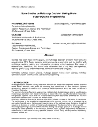
- 5. P.K.Parida, S.K.Sahoo, K.C.Sahoo International Journal of Logic and Computation (IJLP), Volume (1): Issue (1) 56 0 C 1 C 2 C 1−N C 0u 1u 2u 1−Nu 0x 1x 2x ...... 1−Nx Nx 0 G 1 G 2 G 1−N G N G 0=t 1=t 2=t 1−= Nt Nt = FIGURE 1: A General Framework For Multistage Decision Making Under Fuzziness The multistage decision making (control) under fuzziness may be depicted in Fig.1. We start from an initial state at stage (time) 0=t , 0x make a decision 0u attain a state, at time 1=t , 1x make a decision 1u ,…… Finally, being at 1−= Nt in 1−Nx , we apply 1−Nu and attain the final state Nx . The state transitions are given Eq.(11), the consecutive decision tu are subjected to fuzzy constraints t C and on the states 1+tx fuzzy goals 1+t G are imposed, .1,.......,1,0 −= Nt The multistage decision making process is evaluated by the fuzzy decision which is assumed a decomposable fuzzy set in XUXU ×××× ....... , is ( ) ( ) ( ) ( ) ( )NGNCGCND xuxuxuuu NN µµµµµ ∧∧∧∧= −− − 1100110 110 ..........,.....,, ( ) ( )[ ]1 1 0 1 + − = +∧∧= tGtC N t xu tt µµ (12) where N is some termination time is fixed. The basic case, the optimal sequence of decisions * 1 * 1 * 0 ,.....,, −Nuuu , such that ( ) ( ) ( ) ( ) ( )[ ]NGNCGCuuu ND xuxuxuuu NN N µµµµµ ∧∧∧∧= −− − − 110 ,...,, 0 * 1 * 1 * 0 110 110 ..........max,.....,, ( ) ( )[ ]1 1 0,...,, 1 110 max + − = + − ∧∧= tGtC N tuuu xu tt N µµ (13) For simplicity, a fuzzy goal, ( )NG xNµ is only imposed on the final state Nx . Then the fuzzy decision is ( ) ( ) ( ) ( ) ( )NGNCGCND xuxuxuuu NN µµµµµ ∧∧∧∧= −− − 1100110 110 ..........,.....,, (14) and the problem is to find * 1 * 1 * 0 ,.....,, −Nuuu , such that System under control S System under control S System under control S
- 6. P.K.Parida, S.K.Sahoo, K.C.Sahoo International Journal of Logic and Computation (IJLP), Volume (1): Issue (1) 57 ( ) ( ) ( ) ( ) ( )[ ]NGNCGCuuu ND xuxuxuuu NN N µµµµµ ∧∧∧∧= −− − − 110 ,...,, 0 * 1 * 1 * 0 110 110 ..........max,.....,, (15) This general problem formulation may be extended, mainly with respect to ([11] and [12]): ● The type of termination time: fixed and specified in advance, fuzzy implicitly given infinite. ● The type of the dynamic system: deterministic, stochastic, fuzzy and fuzzy stochastic. ● The type of objective function: cost minimization, profit/benefit maximization and fuzzy criterion set based satisfactory degree maximization, and virtually all cases a dynamic- programming-type algorithm can be devised. 4. FUZZY DYNAMIC PROGRAMMING FOR THE CASE OF A FIXED AND SPECIFIED TERMINATION TIME The case of a fixed and specified (in advance) termination time is basic, and provides a suitable point of departure for extensions. Here we discussed a deterministic, stochastic, fuzzy dynamic system, and fuzzy criterion set dynamic program. 4.1. THE CASE OF A DETERMINISTIC DYNAMIC SYSTEM A deterministic system is described by its state transition Eq.(11), i.e. ( )ttt uxfx ,1 =+ ; { }ntt sssXxx ,......,,, 211 =∈+ ; { }mt cccUu ,........,, 21=∈ ; 1,......,1,0 −= Nt , Xx ∈0 is the initial state, and ∞<N is a fixed and specified termination time. The fuzzy constraints are ( ) ( )10 10 .,,......... −− NCC uu Nµµ and the fuzzy goal is ( )NG xNµ . The fuzzy decision is ( ) ( ) ( ) ( )NGNCCND xuuxuuu NN µµµµ ∧∧∧= −− − 100110 10 ..........,.....,, (16) and to find * 1 * 1 * 0 ,.....,, −Nuuu , such that ( ) ( ) ( ) ( )[ ]NGNCCuuu ND xuuxuuu NN N µµµµ ∧∧∧= −− − − 10 ,...,, 0 * 1 * 1 * 0 10 110 ..........max,.....,, (17) Clearly, the last two terms are ( ) ( )( )111 ,1 −−− ∧− NNGNC uxfu NN µµ depend on 1−Nu , hence Eq.(17) can be rewritten as ( ) ( ) ( ) ( )[ ]NGNCCuuu ND xuuxuuu NN N µµµµ ∧∧∧= −− − − 10 ,...,, 0 * 1 * 1 * 0 10 110 ..........max,.....,, ( ) ( ) ( ) ( )( )( ) ∧∧∧∧= −−−− − − − − 11120 ,...,, ,max.....max 1 1 20 110 NNGNCu NCCuuu uxfuuu NN N N N µµµµ (18)
- 7. P.K.Parida, S.K.Sahoo, K.C.Sahoo International Journal of Logic and Computation (IJLP), Volume (1): Issue (1) 58 On repeating this backward iteration for 021 ,.....,, uuu NN −− , we obtain the set of dynamic programming recurrence equations ( ) ( ) ( )[ ] ( ) == ∧= −−+− +−−− +−− − − Niuxfx xux iNiNiN iNGiNCu iNG iNiN iN iN ,........,2,1,, max 1 11µµµ (19) where ()⋅−iN G µ is a fuzzy goal at iNt −= induced by a fuzzy goal at 1+−= iNt . An optimal sequence of decisions sought, * 1 * 1 * 0 ,.....,, −Nuuu is given by the successive maximizing values of iNu − in Eq.(19). It is convenient to represent the solution, * tu , by an optimal policy UXat →:* , such that ( )ttt xau ** = , 1,........,1,0 −= Nt , i.e., relating an optimal decision to the current state. 4.2. THE CASE OF A STOCHASTIC DYNAMIC SYSTEM The stochastic system is assumed to be a Markov chain whose temporal evolution is described by a conditional probability ( )ttt uxxP ,1+ such that { }ntt sssXxx ,......,,, 211 =∈+ , { }mt cccUu ,........,, 21=∈ ; Xx ∈0 is an initial state, 1,......,1,0 −= Nt and ∞<N is a fixed and specified termination time. Now the following two problem formulations: ● due to [19]: find an optimal sequence of decisions * 1 * 1 * 0 ,.....,, −Nuuu to maximize the probability of attainment of the fuzzy goal, subject to the fuzzy constraints, i.e. ( ) ( ) ( ) ( )[ ]NGNCCuuu ND xuuxuuu NN N µµµµ ∧∧∧= −− − − 10 ,...,, 0 * 1 * 1 * 0 10 110 ..........max,.....,, (20) where the fuzzy goal is viewed to be a fuzzy event in X whose (non-fuzzy) probability is [17], ( ) ( ) ( )∑∈ −−= Xx NGNNNNG N NN xuxxPxE µµ ., 11 (21) ● due to [14]: find an optimal sequence of decisions * 1 * 1 * 0 ,.....,, −Nuuu to maximize the expectation of the fuzzy decisions membership function, i.e. ( ) ( ) ( ) ( )[ ]NGNCCuuu ND xuuExuuu NN N µµµµ ∧∧∧= −− − − 10 ,...,, 0 * 1 * 1 * 0 10 110 ..........max,.....,, (22) These formulations are clearly not equivalent. Bellman and Zadeh’s approach [19] Since in Eq.(20), ( ) ( )[ ]111 ,1 −−− ∧− NNGNC uxfEu NN µµ depend only on 1−Nu , the next two right-most terms depend only on 2−Nu etc., the structure of Eq.(20) is essentially the same as that of Eq.(18), and the set of fuzzy dynamic programming recurrence equation is ( ) ( ) ( )[ ] ( ) ( ) ( ) == ∧= ∑∈ +−−−+−+− +−−− +− +−+− +−− − − NixuxxPxE xEux Xx iNGNNiNiNG iNGiNcu iNG iN iNiN iNiN iN iN ,....,2,1;, max 1 11 1 11111 1 µµ µµµ (23)
- 8. P.K.Parida, S.K.Sahoo, K.C.Sahoo International Journal of Logic and Computation (IJLP), Volume (1): Issue (1) 59 and we consecutively obtain * iNu − or optimal policies * iNa − , such that ( )iNiNiN xau −−− = ** , Ni ,.......,2,1= . Kacprzyk and Staniewski’s approach [14] To solve problem Eq.(22), first introduce a sequence of functions [ ]1,0: 1 →× = UXXh i j i and [ ]1,0: 1 1 →× + = UXXg j l j ; Ni ,......,2.1,0= ; 1,.......,2,1 −= Nj , such that ( ) ( ) ( ) ( ) ( ) ( ) ( ) ( ) ( ) ( ) ( ) = = = ∧∧∧= − = + −−− ∑ − 00000 010 1 010 0101010 ,max ............................................................................................................. ,........,,max,........,, ,.,........,,,........,, ............................................................................................................ ,.....,.....,,........., 0 10 uxgxh uuxguuxh uxsPuushuuxg xuuuuuuxh u kkk u kkk n i kkikikkkk NDNCCNNN k N µµµ (24) The consecutive decisions and states are juuu ,........,, 10 and jxxx ,........,, 10 , respectively, then jg is the expected value of ( )0xD ⋅µ provided that the next decisions are optimal, i.e. * 1 * 2 * 1 ,........,, −++ Njj uuu . It can be shown ([11], [12] and [14]), that there exist functions UUXX k j k →× =1 :ω , such that ( ) ( )( )101010 ,........,,,,........,,,........,, −−− = kkkkkkkkk uuxuxguuxh ωω . Then, an optimal policy sought, * ta , 1,.......,2,1,0 −= Nt is given by ( ) ( ) ( )( ) ( ) ( )( )( ) = = = −−−−−− ,......,.......,,.......,,,......,, ......................................... ,, 0 * 020 * 211110 * 1 0 * 01110 * 1 00 * 0 xaxxaxxxxa xaxxxa xa NNNNNN ω ω ω (25) It is depends not only on the current state but also on the trajectory. 4.3. THE CASE OF A FUZZY DYNAMIC SYSTEM In this case the system is fuzzy and its dynamics is governed by a state transitions equation ( )ttt UXFX ,1 =+ , ,.........2,1,0=t (26)
- 9. P.K.Parida, S.K.Sahoo, K.C.Sahoo International Journal of Logic and Computation (IJLP), Volume (1): Issue (1) 60 where tX , 1+tX are fuzzy states at time (stage) t and 1+t , and tU is a fuzzy decision at t characterized by their membership functions ( )tX xt µ , ( )11 ++ tX xt µ and ( )tU ut µ , respectively. Eq.(26) is equivalent to a conditioned fuzzy set ( )tttX uxxt ,11 ++ µ ([11] and [12]). Baldwin and Pilsworth [13] proposed a dynamic programming scheme. First, for each 1,,.........2,1,0 −= Nt a fuzzy relation ( ) ( ) ( )11 1, ++ +∧= tGtCttR xuxu ttt µµµ is constructed. The degree to which tU and 1+tX satisfy t C and 1+t G is ( )( ) ( ) ( )( ) ( ) ( )( ) ∧∧∧= ++++ + + + 1111 1 1 1 maxmax,,, tGtX x tCtU u tttRtT xxuuxxuu t t t t t t t µµµµµµ (27) The fuzzy decision is ( )010 ,........, XUU ND −µ ( ) ( )( ) ( ) ( )( ) ( ) ( )( ) ∧∧∧∧∧∧= −− − − − NGNX x NCNU uCU u xxuuuu N N N N N N µµµµµµ maxmax.......max 1100 1 1 1 0 0 0 (28) and an optimal sequence of fuzzy decisions * 1 * 0 ,........, −NUU , such that ( ) ( )010 ,....., 0 * 1 * 0 ,........,max,........, 10 XUUXUU ND UU ND N −− − = µµ ( ) ( )( ) ( ) ( ) ( ) ( )( ) ∧ ∧∧ ∧∧∧= −− − − −− NGNX xX NCNU uUCU uU xx uu uu N N NN N N NN µµ µµ µµ maxmax maxmax.......maxmax 11 00 1 1 11 0 0 00 (29) Hence the set of dynamic programming recurrence equation is ( ) ( ) ( )[ ] ( ) ( ) ( )( ) ( ) ( ) ( ) ( )( ) ( ) −= ∧ ∧= ∧∧= ∧= −−−+−−+− +−−−− −+−− −− +− +−− − −− − 1,........,2,1 ,maxmax maxmax max 11 1 1 1 1 1 1 Ni xuxxux XuuX xxX iNXiNiNiNXiNU ux iNX iNGiNCiNU uU iNG NGNX x NG iNiNiN NiN iN iNiN iN NiN iN N N N N µµµµ µµµµ µµµ (30) They redefine the problem formulation in terms of the reference fuzzy states and fuzzy decisions to finally make Eq.(30) solvable ([11], [12] and [13]). 5. FUZZY DYNAMIC PROGRAMMING FOR THE CASE OF A FUZZY TERMINATION TIME In many real-world problems it may be more adequate (sufficient) to assume a fuzzy termination time as more or less 5 years, a couple of days, ten years or so [7].
- 10. P.K.Parida, S.K.Sahoo, K.C.Sahoo International Journal of Logic and Computation (IJLP), Volume (1): Issue (1) 61 Let { }NkkkR ,.......,1,,1,......,1,0 +−= be the set of decision making states. At each Rt ∈ , a fuzzy constraint ( )tC utµ , and a fuzzy goal ( )vG xvµ , Rv∈ is imposed on the final state. The fuzzy termination time is given by ( )vTµ , Rv ∈ , which is a termination time v . The fuzzy decision ( ) ( ) ( ) ( ) ( )vGTvCCvD xvuuxuuu vv µµµµµ ...........,.....,, 100110 10 ∧∧∧= −− − (31) and to find an optimal termination time * v and an optimal sequence of decisions * 1 * 1 * 0 ,.....,, −vuuu such that ( ) ( ) ( ) ( ) ( )[ ]vGTvCCuuu vD xvuuxuuu vv N µµµµµ ...........max,.....,, 10 ,...,, 0 * 1 * 1 * 0 10 110 ∧∧∧= −− − − (32) 5.1. THE CASE OF A DETERMINISTIC DYNAMIC SYSTEM Eq.(32) was formulated and solved by Kacprzyk ([7] and [8]). Then, Stein [23] presented a computationally more efficient model and solution. Kacprzyk’s approach In Kacprzyk’s ([7] and [9]) formulation the set of possible termination times is ( ){ } { } RNkkvRv T ⊆+=>∈ ,.......,1,0: µ , hence an optimal sequence of decisions is * 1 ** 1 * 1 * 0 ,....,,,.....,, −− vkk uuuuu . The part * 1 ** 1 *,....,, −− vkk uuu is determined by solving ( ) ( ) ( )[ ] ( ) −+=+−= = ∧= −−+− +−−− +−− − − 1,......,1,;1,......,2,1 , ,max, 1 11 Nkkvivi uxfx vxuvx iviviv ivGivCV ivG iviv iv iv µµµ (33) where ( ) ( ) ( )vGTvG xvvx vv µµµ ., = . An optimal termination time * v , then found by the maximizing v in ( ) ( )vxx kGv kG kk ,max 11 11 −− −− = µµ (34) The part * 2 * 1 * 0 ,.....,, −Kuuu is then determined by solving ( ) ( ) ( )[ ] ( ) −== ∧= −−−−− −−−+− −−− −− +− 1,.......,2,1;, max 11 11 1 1 1 kiuxfx xux ikikik ikGikCu ikG ikik ik ik µµµ (35) Stein’s approach Stein [23] presented a computationally more efficient dynamic programming approach. At 1−= Nt , { }1,......,2,1 −∈ Ni , and attain ( ) ( ) ( )iNGTiNG xiNx iNiN −− −− −= µµµ . or apply iNu − and attain ( ) ( )11 +−− +−− ∧ iNGiNC xu iNiN µµ . The set of recurrence equation is therefore
- 11. P.K.Parida, S.K.Sahoo, K.C.Sahoo International Journal of Logic and Computation (IJLP), Volume (1): Issue (1) 62 ( ) ( ) ( ) ( )[ ] ( ) == ∧= −−+− +−−−− +−− − − − Niuxfx xuxx iNiNiN iNGiNCu iNGiNG iNiN iN iN iN ,.......,2,1;, max 1 11µµµµ (36) and an optimal termination time is such a iNt −= at which terminating decision * 1* −v u , occurs, i.e. when ( ) ( ) ( )[ ]11max +−−− +−− − − ∧> iNGiNCu iNG xux iNiN iN iN µµµ (37) 5.2. THE CASE OF A STOCHASTIC DYNAMIC SYSTEM This stochastic dynamic system was first formulated and solved in Kacprzyk ([8] and [9]) by combining the section 4.2 and 5.1. An optimal termination time * v and an optimal sequence of decisions * 1 * 1 * 0 ,.....,, −vuuu such that ( ) ( ) ( ) ( )[ ]vGvCCuuuv vD xEuuxuuu vv v µµµµ ∧∧∧= −− − − 10 ,...,,, 0 * 1 * 1 * 0 10 110 ..........max,.....,, (38) where ( ) ( ) ( )vGTvG xvx vv µµµ .= ; and ( ){ } { }Nkkvv T ,......,1,0: +=>µ . As in section 4.2, we determine * v and * 1 ** 1 *,....,, −− vkk uuu by solving ( ) ( ) ( )[ ] ( ) ( ) ( ) =×= ∧= +− ∈ −−+−+− +−−− +− +− +− +−− − − ∑ NixuxxPxE xEux ivG Xx vvivivG ivGivCu ivG iv iv iv iviv iv iv ,.....,2,1;, max 11111 1 1 1 1 1 µµ µµµ (39) and * v is given by the maximizing v in ( ) ( )vxx kGv kG kk ,max 11 11 −− −− = µµ (40) The remaining part * 0 * 3 * 2 ,.....,, uuu kk −− is obtained by solving ( ) ( ) ( )[ ] ( ) ( ) ( ) −=×= ∧= ∑∈ −−−−−−−− −−−−− − −−− −−− −− −− 1,.......,2,1;, max 111 11 1 1 1 1 kixuxxPxE xEux Xx ikGikikikikG ikGikCu ikG ik ikik ikik ik ik µµ µµµ (41) In the later Stein’s [23], formulation the problem is solved by the following set of recurrence equations ( ) ( ) ( ) ( )[ ] ( ) ( ) ( )( ) =×= ∧∧= ∑∈ −−−−+−+− +−−−− − +−+− +−− − − − NiuxfuxxPxE xEuxx Xx iNiNGiNiNiNiNG iNGiNCu iNGiNG iN iNiN iNiN iN iN iN ,.......,2,1;,, max 11 1 11 1 µµ µµµµ (42) where * v occurs when ( ) ( ) ( )[ ]11max +−−− +−− − − ∧> iNGiNCu iNG xEux iNiN iN iN µµµ (43)
- 12. P.K.Parida, S.K.Sahoo, K.C.Sahoo International Journal of Logic and Computation (IJLP), Volume (1): Issue (1) 63 5.3. THE CASE OF A FUZZY DYNAMIC SYSTEM In this case, fix some (finite and relatively small) number of reference fuzzy states (and possibly decisions), and obtain an auxiliary approximate system whose state transitions are of deterministic system type ([12] and [16]). Then, Stein’s [23] approach can be employed. 6. MULTISTAGE DECISION MAKING (CONTROL) WITH AN IMPLICIT SPECIFIED TERMINATION TIME Now the process terminates when the state enters for the first time a termination set of states { } XsssW npp ⊂= ++ ,......,, 21 . We determine an optimal sequence of decisions * 1 * 1 * 0 ,........,, −N uuu , such that ( )0 * 1 * 1 * 0 ,........,, xuuu ND − µ ( ) ( ) ( )]..........[max 1100 ,...,, 110 NGNNCC uuu xxuxu N N µµµ ∧∧∧= −− − (44) where Xxxx N ∈−110 ,.....,, W , and WxN ∈ The solution of Eq.(44) may proceed by using: ● Bellman and Zadeh’s [19] iterative approach, ● Komolov’s et al. [22] graph theoretic approach and ● Kacprzyk’s ([5] and [8]) branch and bound approach. 7. MULTISTAGE DECISION MAKING (CONTROL) WITH AN INFINITE TERMINATION TIME In all the problems considered the solution process required some iteration over consecutive stages. This may be justified the number of stages is not too high, and when the process itself exhibits a sufficient variability over time. In the fuzzy setting, the multistage decision making (control) problem with an infinite termination time was first formulated and solved by Kacprzyk and Staniewski ([15] and [16]). For the deterministic dynamic system Eq.(11), the fuzzy decision is ( ) ( ) ( ) ( ) ( ) ..........,......., 211100010 ∧∧∧∧= xxuxxuxuu GCGCD µµµµµ ( ) ( )[ ]1 0 lim + =∞→ ∧∧= tGttC N tN xxu µµ (45) and to find an optimal stationary strategy ( ),........., *** aaa =∞ , such that ( ) ( )00 * max xaxa D a D ∞∞ ∞ = µµ ( )( ) ( )[ ]1 0 limmax + =∞→ ∧∧= ∞ tGttC N tNa xxxa µµ (46) Eq.(46) may be solved in a finite number of steps by using a policy iteration algorithm whose essence is a step-by-step improvement of stationary policies. A policy iteration type algorithm was also proposed for the stochastic system by [16].
- 13. P.K.Parida, S.K.Sahoo, K.C.Sahoo International Journal of Logic and Computation (IJLP), Volume (1): Issue (1) 64 8. COMPUTATIONAL COMPLEXITY The development of efficient algorithms for processing various aspects of fuzzy dynamic programs is an important research area in dynamic programming. In this section, we will summarize main results of the computational complexity analysis provided by (1997). Esogbue [2] using two algorithms of Kacprzyk [7] and Stein [23] for the fuzzy termination time discussed. Esogbue showed that the dynamic programming approach presented by Kacprzyk requires ( ) 2/1+NN iterations while the one proposed by Stein [23] requires only N and it is computationally more efficient. Let, the time and space complexity analysis for both. Here, consisting of n equations and 1−Nu controls each assuming m values, and time kNt ,.......,1−= , the total number of operations involved is ( ) ( ) ( ) ( )12..11222 −−++−++−−− mnkkNnktmmkmtn (47) Let tkm == , then Eq.(47) is of order ( )3 2 kO . The basic dynamic programming formulation of the problem proposed by Stein [23] is the same expect for the structure of the recurrence equations that require N only iterations of the optimizing process as opposed to ( ) 2/1+NN required is Kacprzyk’s algorithm. The space and the time complexities are of order ( )nO and ( )mnO , respectively. Essentially, the time complexity is of order ( )( )( )kNmO −− 12 . This is of order ( )2 kO . The total storage demand is ( )( ) ( )122/21 −+++−+− knnkNkNn . This is order ( )kO . It was pointed out, the difference between the earliest and the latest possible termination times is an important factor in the computationally burden of this optimization process. So, the model proposed by Stein [23] is computationally more efficient, taking ( )kO memory spaces in ( )2 kO operations, as opposed to ( )2 kO memory spaces in ( )3 kO operations in Kacprzyk’s (1977) model. The superiority is exhibited both from the space and time complexity considerations. The case of stochastic system, it was shown that the computational burden and storage requirements are identical for both algorithms. If in the dynamic programming formulation, the objective is to maximize the probability of attainment of the fuzzy goal G subject to non fuzzy constraints. 9. CONCLUSION We have presented a brief exposition of main aspects of fuzzy dynamic programming, including main problem classes and major applications in a variety of fields. We have studied dynamic programming problems in fuzzy environments. Some basic problems have been studied and development of fuzzy dynamic programming is given. It is shown that the fuzzy dynamic programming may be a promising tool for dealing with multistage decision making and optimization problems under fuzziness. For other surveys of fuzzy dynamic programming and its applications, we refer the reader to [1] and then the fundamental presentation by [6] and [11]. REFERENCE [1] A.O. Esogbue and R.E. Bellman. “Fuzzy dynamic programming and its extensions”. TIMS/ Studies in the Management Sciences, 20, 147-167, 1984. [2] A.O. Esogbue and V. Ramesh. “Dynamic Programming and fuzzy allocation processes”. Technical Memo No. 202, Dept. of Operation Research Case Western University, Cleveland, OH., (1970).
- 14. P.K.Parida, S.K.Sahoo, K.C.Sahoo International Journal of Logic and Computation (IJLP), Volume (1): Issue (1) 65 [3] G. Conrnuejds and R. Tutuncu. “Optimization Methods in Finance”. Cambride University Press, (2007). [4] H.-J. Zimmermann. “Fuzzy Sets, Decision Makings, and Experts Systems”. Kluwer, Dordrecht (1987). [5] J. Kacprzyk. “A branch-and-bound algorithm for the multistage control of a non fuzzy system in a fuzzy environment”. Control and Cybernetices, 7, 51-64, 1978b. [6] J. Kacprzyk. “A generalization of fuzzy multistage decision making and control via linguistic quantifiers”. Int. J. of Control, 38, 1249-1270, 1978b. [7] J. Kacprzyk. “Control of non-fuzzy system in a fuzzy environment with fuzzy termination time”. Systems Sciences, 3, 325-341, 1977. [8] J. Kacprzyk. “Control of a stochastic system in a fuzzy enviroment with fuzzy termination time”. Systems Science, 4, 291-300, 1978b. [9] J. Kacprzyk. “Decision making in a fuzzy environment with fuzzy termination time”. Fuzzy Sets and Systems, 1, 169-179, 1978b. [10] J. Kacprzyk. “Fuzzy dynamic programming: A new quality through fuzzy sets”. In Da Ruan (Ed). Fuzzy Sets Theory and Advanced Mathematical applications, Kluwer, Dordrecht, 137-154, 1996. [11] J. Kacprzyk. “Multistage control: A model based approach to control and decision making”. Wiley, Chichester (1997). [12] J. Kacprzyk. “Multistage decision making under fuzziness”. Verlag TUV, Rheinland, Cologne (1978b). [13] J.F. Baldwin and B.W. Pilsworth. “Dynamic programming for fuzzy systems with fuzzy environment”. J. Math. Anal. and Apples., 85, 1-23, 1982. [14] J. Kacprzyk and P. Staniewski. “A new approach to the control of stochastic systems in a fuzzy environment”. Arch. Automat, Telemech, XXV, 443-444, 1980. [15] J. Kacprzyk and P. Staniewski. “Control of a deterministic system in a fuzzy environment over an infinite planning horizon”. J. of Fuzzy Sets and Systems 10, 291-298, 1983. [16] J. Kacprzyk and P. Staniewski. “Long-term inventory policy-making through fuzzy decision- making models”. J. of Fuzzy Sets and Systems, 8, 117-132, 1982. [17] L.A. Zadeh. “Probability measures of fuzzy events”. J. of math. Anal. And Appls., 23, 421-427, 1968. [18] R.E. Bellman. “Dynamic programming”. Princeton Univ. Press, Princeton, NJ.
- 15. P.K.Parida, S.K.Sahoo, K.C.Sahoo International Journal of Logic and Computation (IJLP), Volume (1): Issue (1) 66 [19] R.E. Bellman and L.A. Zadeh. “Decision-making in a fuzzy environment”. Management Sci., 17, 141-164, 1970. [20] R. Brorson and G. Naadimuthu. “Theory and Problems of Operations Research”. (2006). [21] S.S.L. Chang. “Fuzzy dynamic programming and the decision making process”. Proc. 3rd Princeton Conf. of Inf. Sci. and Syst. (Princeton, NJ, USA), 200-203, 1969. [22] S.V. Komolov et al. “On the problem of optimal control of a finite automaton with fuzzy constraints and fuzzy goal (in Russian)”. Kybernetika (Kiev), 6, 30-34, 1979. [23] W.E. Stain. “Optimal stopping in a fuzzy environment”. J. of Fuzzy Sets and Systems, 3, 252-259, 1968. [24] Y. Yoshida. “Dynamical Aspects in Fuzzy Decision Making”. pp.1-25, (2001).