1. The Astrophysical Journal, 781:121 (20pp), 2014 February 1
C
doi:10.1088/0004-637X/781/2/121
2014. The American Astronomical Society. All rights reserved. Printed in the U.S.A.
THIRD-EPOCH MAGELLANIC CLOUD PROPER MOTIONS. II. THE LARGE MAGELLANIC
CLOUD ROTATION FIELD IN THREE DIMENSIONS
1
Roeland P. van der Marel1 and Nitya Kallivayalil2,3,4
Space Telescope Science Institute, 3700 San Martin Drive, Baltimore, MD 21218, USA
2 Yale Center for Astronomy & Astrophysics, 260 Whitney Avenue, New Haven, CT, USA
Received 2013 May 14; accepted 2013 December 10; published 2013 January 16
ABSTRACT
We present the first detailed assessment of the large-scale rotation of any galaxy based on full three-dimensional
velocity measurements. We do this for the LMC by combining our Hubble Space Telescope average proper motion
(PM) measurements for stars in 22 fields, with existing line-of-sight (LOS) velocity measurements for 6790
individual stars. We interpret these data with a model of circular rotation in a flat disk. The PM and LOS data paint
a consistent picture of the LMC rotation, and their combination yields several new insights. The PM data imply
a stellar dynamical center that coincides with the H i dynamical center, and a rotation curve amplitude consistent
with that inferred from LOS velocity studies. The implied disk viewing angles agree with the range of values found
in the literature, but continue to indicate variations with stellar population and/or radius. Young (red supergiant)
stars rotate faster than old (red and asymptotic giant branch) stars due to asymmetric drift. Outside the central
region, the circular velocity is approximately flat at Vcirc = 91.7 ± 18.8 km s−1 . This is consistent with the baryonic
Tully–Fisher relation and implies an enclosed mass M(8.7 kpc) = (1.7 ± 0.7) × 1010 M . The virial mass is larger,
◦
◦
depending on the full extent of the LMC’s dark halo. The tidal radius is 22.3 ± 5.2 kpc (24. 0 ± 5. 6). Combination
of the PM and LOS data yields kinematic distance estimates for the LMC, but these are not yet competitive with
other methods.
Key words: galaxies: individual (Large Magellanic Cloud) – galaxies: kinematics and dynamics –
Magellanic Clouds – proper motions
Online-only material: color figures
2011; Sohn et al. 2013; Boylan-Kolchin et al. 2013). More recently it has even become possible to go out as far as M31
(Sohn et al. 2012; van der Marel et al. 2012a, 2012b). All of
these studies have aimed at measuring the systemic center-ofmass (COM) motion of the target galaxies, and not their internal
kinematics. So typically, only one to three different fields were
observed in any given galaxy. By contrast, a study of internal
kinematics requires, in addition to high PM accuracy, a larger
number of different fields spread out over the face of the galaxy.
In K06, we presented a detailed PM study of the LMC. We
used HST to observe 21 fields centered on background quasars,
in two epochs separated by a median baseline of 1.9 yr. The
distribution of observed fields extends to 4◦ from the LMC
center (1◦ = 0.87 kpc for an assumed distance of 50.1 kpc,
i.e., m − M = 18.50; Freedman et al. 2001). From the data we
derived the average PM of the stars in each field. We used this
to estimate the PM of the LMC COM. In Besla et al. (2007),
our team studied the implied orbit of the Magellanic Clouds and
argued that they may be falling into the Milky Way for the first
time. The data also allowed us to detect the PM rotation of the
LMC at 1.3σ significance. The rotation sense and magnitude
were found to be consistent with the detailed predictions for the
LMC PM rotation field presented by van der Marel et al. (2002,
hereafter vdM02), based on the observed LOS rotation field of
carbon stars.
Piatek et al. (2008, hereafter P08) performed a more sophisticated reanalysis of our K06 data, including small corrections
for charge-transfer efficiency (CTE) losses. This yielded better
PM consistency between fields, but implied a similar PM for
the LMC COM. P08 used their measurements to derive the first
crude PM rotation curve for the LMC, assuming fixed values
for the dynamical center and disk orientation. However, their
1. INTRODUCTION
Measurements of galaxy rotation curves form the foundation
of much of our understanding of galaxy formation, structure, and
dynamics (e.g., Binney & Merrifield 1998; Binney & Tremaine
2008; Mo et al. 2010). The current knowledge of galaxy rotation
is based entirely on observations of Doppler shifts in radiation
from galaxies. This yields only one coordinate of motion, the
line-of-sight (LOS) velocity. If a galaxy rotates, and is not
viewed edge-on, it will also rotate in the plane of the sky. Until
now, the implied proper motions (PMs) have generally been
undetectable, given the available observational capabilities.
However, the observational capabilities have steadily advanced.
We present here new results for the LMC that constitute the first
detailed measurement and analysis of the large-scale rotation
field of any galaxy in all three dimensions.5
The Hubble Space Telescope (HST) provides a unique combination of high spatial resolution, long-term stability, exquisite
instrument calibrations, and ever-increasing time baselines.
Over the past decade, this has opened up the Local Group of
galaxies to detailed PM studies. These studies have focused primarily on the satellites of the Milky Way (Kallivayalil et al.
2006b, hereafter K06; Kallivayalil et al. 2006a; Piatek & Pryor
2008 and references therein; Pryor et al. 2010; L´ pine et al.
e
3
YCAA Prize Fellow.
Also at Department of Astronomy, University of Virginia, 530 McCormick
Road, Charlottesville, VA 22904, USA.
5 VLBI observations of water masers have been used to detect the PM
rotation of nuclear gas disks in some galaxies (e.g., NGC 4258; Herrnstein
et al. 1999). Similar techniques can in principle be used to study the
large-scale rotation curve of nearby galaxies (e.g., Brunthaler et al. 2005), but
this has not yet been explored in detail.
4
1

2. The Astrophysical Journal, 781:121 (20pp), 2014 February 1
van der Marel & Kallivayalil
inferred rotation amplitude Vrot = 120 ± 15 km s−1 appears too
high, exceeding the known rotation of cold H i gas (Kim et al.
1998; Olsen & Massey 2007) by ∼40 km s−1 . So better data are
needed to accurately address the PM rotation of the LMC.
We recently presented a third epoch of HST PM data for 10
fields (Kallivayalil et al. 2013, hereafter Paper I), increasing the
median time baseline to 7.1 yr. For these fields we obtained a
median per-coordinate random PM uncertainty of only 7 km s−1
(0.03 mas yr−1 ), which is a factor 3–4 better than in K06 and
P08. This corresponds to ∼10% of the LMC rotation amplitude.
As we show in the present paper, these data are sufficient to
map out the LMC PM rotation field in detail, yielding new
determinations of the LMC dynamical center, disk orientation,
and rotation curve.
Several interesting ground-based LMC PM measurements
have also been published in recent years (e.g., Costa et al. 2009;
Vieira et al. 2010; Cioni et al. 2013). Such measurements hold
the future promise to allow PM measurements over a much
larger area of the LMC than is possible with the HST, and for
different stellar populations. However, to date these studies are
not yet competitive with the HST for analysis of the LMC PM
rotation field in terms of either PM accuracy or spatial coverage
(see, e.g., Section 4.2 of Paper I).
The LMC is a particularly interesting galaxy for which to
perform a study of the PM rotation field. At a distance of
only ∼50 kpc, it is one of nearest and best-studied galaxies
next to our own Milky Way (e.g., Westerlund 1997; van
den Bergh 2000). It is a benchmark for studies on various
topics, including stellar populations and the interstellar medium,
microlensing by dark objects, and the cosmological distance
scale. As nearby companion of the Milky Way, with significant
signs of interaction with the Small Magellanic Cloud (SMC),
the LMC is also an example of ongoing hierarchical structure
formation. For all these applications it is important to have a
solid understanding of the LMC structure and kinematics.
The current state of knowledge about the kinematics of the
LMC was reviewed recently by van der Marel et al. (2009).
Studies of the LOS velocities of many different tracers have
contributed to this knowledge. The kinematics of gas in the
LMC has been studied primarily using H i (e.g., Kim et al.
1998; Olsen & Massey 2007; Olsen et al. 2011, hereafter O11).
Discrete LMC tracers which have been studied kinematically
include star clusters (e.g., Schommer et al. 1992; Grocholski
et al. 2006), planetary nebulae (Meatheringham et al. 1988),
H ii regions (Feitzinger et al. 1977), red supergiants (Prevot
et al. 1985; Massey & Olsen 2003; O11), red giant branch
(RGB) stars (Zhao et al. 2003; Cole et al. 2005; Carrera et al.
2011), carbon stars and other asymptotic giant branch (AGB)
stars (e.g., Kunkel et al. 1997; Hardy et al. 2001; vdM02; Olsen
& Massey 2007; O11), and RR Lyrae stars (Minniti et al. 2003;
Borissova et al. 2006). For the majority of tracers, the line-ofsight velocity dispersion is at least a factor of around two smaller
than their rotation velocity. This implies that on the whole the
LMC is a (kinematically cold) disk system.
Specific questions that can be addressed in a new way through
a study of the LMC PM rotation field include the following.
1. What is the stellar dynamical center of the LMC, and does
this coincide with the H i dynamical center? It has long
been known that different measures of the LMC center
(e.g., center of the bar, center of the outer isophotes, H i
dynamical center, etc.) are not spatially coincident (e.g.,
van der Marel 2001, hereafter vdM01; Cole et al. 2005),
but a solid understanding of this remains lacking.
2. What is the orientation under which we view the LMC disk?
Past determinations of the inclination angle and the line-ofnodes position angle have spanned a significant range, and
the results from different studies are often not consistent
within the stated uncertainties (e.g., van der Marel et al.
2009). Knowledge of the orientation angles is necessary
to determine the face-on properties of the LMC, with past
work indicating that the LMC is not circular in its disk plane
(vdM01).
3. What is the PM of the LMC COM, which is important
for understanding the LMC orbit with respect to the
Milky Way? We showed in Paper I that the observational
PM errors are now small enough that they are not the
dominant uncertainty anymore. Instead, uncertainties in our
knowledge of the geometry and kinematics of the LMC disk
are now the main limiting factor.
4. What is the rotation curve amplitude of the LMC? Previous
studies that used different tracers or methods sometimes
obtained inconsistent values (e.g., P08; O11). The rotation
curve amplitude is directly tied to the mass profile of the
LMC, which is an important quantity for our understanding
of the past orbital history of the LMC with respect to the
Milky Way (Paper I).
5. What is the distance of the LMC? Uncertainties in this
distance form a key limitation in our understanding of the
Hubble constant (e.g., Freedman et al. 2001). Comparison
of the PM rotation amplitude (in mas yr−1 ) and the LOS
rotation amplitude (in km s−1 ) can in principle yield
a kinematical determination of the LMC distance that
bypasses the stellar evolutionary uncertainties inherent to
other methods (Gould 2000; van der Marel et al. 2009).
In Paper I of this series, we presented our new third epoch
observations, and we analyzed all the available HST PM data for
the LMC (and the SMC). We included a reanalysis of the earlier
K06/P08 data, with appropriate corrections for CTE losses. We
used the data to infer an improved value for the PM and the
galactocentric velocity of the LMC COM, and we discussed the
implications for the orbit of the Magellanic Clouds with respect
to the Milky Way (and in particular whether or not the Clouds
are on their first infall).
In the present paper, we use the PM data from Paper I to study
the internal kinematics of the LMC. The outline of this paper is
as follows. Section 2 discusses the PM rotation field, including
both the data and our best-fit model. Section 3 presents a new
analysis of the LOS kinematics of LMC tracers available from
the literature. By including the new constraints from the PM
data, this analysis yields a full three-dimensional view of the
rotation of the LMC disk. Section 4 discusses implications of
the results for our understanding of the geometry, kinematics,
and structure of the LMC. This includes discussions of the
galaxy distance and systemic motion, the dynamical center and
rotation curve, the disk orientation and limits on precession
and nutation, and the galaxy mass. We also discuss how the
rotation of the LMC compares to that of other galaxies. Section 5
summarizes the main conclusions.
2. PROPER MOTION ROTATION FIELD
2.1. Data
We use the PM data presented in Table 1 of Paper I as the
basis of our study. The data consist of positions (α, δ) for 22
fields, with measured PMs (μW , μN ) in the west and north
directions, and corresponding PM uncertainties (ΔμW , ΔμN ).
2

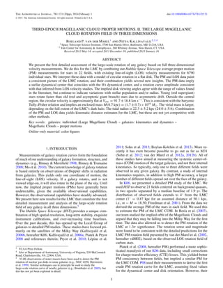
3. The Astrophysical Journal, 781:121 (20pp), 2014 February 1
van der Marel & Kallivayalil
-64
-66
-68
-70
-72
-74
90
80
70
RA
Figure 1. Spatially variable component μobs,var of the observed LMC PM field. The positions of 22 fields observed with HST are indicated by solid dots. The PM
vector shown for each field corresponds to the mean observed absolute PM of the stars in the given field, minus the constant vector μ0 shown in the inset on the bottom
left. The vector μ0 is our best-fit for the PM of the LMC COM (see Table 1 and Paper I). PMs are depicted by a vector that starts at the field location, with a size that
(arbitrarily) indicates the mean predicted motion over the next 7.2 Myr. Clockwise motion is clearly evident. The uncertainty in each PM vector is illustrated by an
open box centered on the end of each PM vector, which depicts the region ±ξ ΔμW by ±ξ ΔμN . The constant ξ = 1.36 was chosen such that the box contains 68.3% of
the two-dimensional Gaussian probability distribution. High-accuracy fields (with long time baselines, three epochs of data, and small error boxes) are shown in red,
while low-accuracy fields (with short time baselines, two epochs of data, and larger error boxes) are shown in green. The figure shows an (RA,DEC) representation of
the sky, with the horizontal and vertical extent representing an equal number of degrees on the sky. The figure is centered on the PM dynamical center (α0 , δ0 ) of the
LMC, as derived in the present paper (see Table 1).
(A color version of this figure is available in the online journal.)
(−1.9103, 0.2292) mas yr−1 . This vector is the best-fit PM of
the LMC COM as derived later in the present paper, and as
discussed in Paper I. Clockwise motion is clearly evident. The
goal of the subsequent analysis is to model this motion to derive
relevant kinematical and geometrical parameters for the LMC.
There are 10 “high-accuracy” fields with long time baselines
(∼7 yr) and three epochs of data,6 and 12 “low-accuracy” fields
with short time baselines (∼2 yr) and two epochs of data. The
PM measurement for each field represents the average PM of
N LMC stars with respect to one known background quasar.
The number of well-measured LMC stars varies by field, but
is in the range 8–129, which a median N = 31. The field size
for each PM measurement corresponds to the footprint of the
HST ACS/HRC camera, which is ∼0.5 × 0.5 arcmin.7 This is
negligible compared to the size of the LMC itself, which extends
to a radius of 10◦ –20◦ (vdM01; Saha et al. 2010).
Figure 1 illustrates the data, by showing the spatially
variable component of the observed PM field, μobs,var ≡
μobs − μ0 , where the constant vector μ0 = (μW 0 , μN0 ) =
2.2. Velocity Field Model
To interpret the LMC PM observations, one needs a model
for the PM vector μ = (μW , μN ) as a function of position on the
sky. The PM model can be expressed as a function of equatorial
coordinates, μmod (α, δ), or as a function of polar coordinates,
μmod (ρ, Φ), where ρ is the angular distance from the LMC
COM and Φ is the corresponding position angle measured from
north over east. Generally speaking, the model can be written
as a sum of two vectors, μmod = μsys + μrot , representing the
contributions from the systemic motion of the LMC COM and
from the internal rotation of the LMC, respectively.
6
This includes one field with a long time baseline for which there is no data
for the middle epoch.
The third-epoch of data was obtained with the WFC3/UVIS camera, which
has a larger field of view. However, the footprint of the final PM data is
determined by the camera with the smallest field of view.
7
3

4. The Astrophysical Journal, 781:121 (20pp), 2014 February 1
van der Marel & Kallivayalil
Consider first the contribution from the systemic motion. The
three-dimensional velocity that determines how the LMC COM
moves through space is a fixed vector. However, the projection
of this vector onto the west and north directions depends on
where one looks in the LMC. This introduces an important
spatial variation in the PM field, due to several different effects,
including: (1) only a fraction cos(ρ) of the LMC transverse
velocity is seen in the PM direction; (2) a fraction sin(ρ) of the
LMC LOS velocity is also seen in the PM direction; and (3) the
directions of west and north are not fixed in a zenithal projection
centered on the LMC, due to the deviation of (α, δ) contours
from an orthogonal grid near the south Galactic pole (see
Figure 4 of van der Marel & Cioni 2001, hereafter vdMC01).
As a result, one can write μsys (α, δ) = μ0 + μper (α, δ). The first
term is the constant PM of the LMC COM, measured at the
position of the COM. The second term is the spatially varying
component of the systemic contribution, which can be referred
to as the “viewing perspective” component.
To describe the component of internal rotation, we assume
that the LMC is a flat disk with circular streamlines. This does
not assume that individual objects must be on a circular orbit, but
merely that the mean motion of every local patch is circular. This
is the same approach that has been used successfully to model
LOS velocities in the LMC (e.g., vdM02; O11). The assumption
is also similar to what is often assumed in the Milky Way, when
one assumes that the LSR follows circular motion. This still
allows for random peculiar motion of individual objects, but we
do not model these motions explicitly. Where relevant, we do
quantify the shot noise introduced by random peculiar motions
(Section 2.5) or the observed velocity dispersion of the random
peculiar motions (Section 3.2).
At any point in the disk, the relation between the transverse
velocity vt in km s−1 and the PM μ in mas yr−1 is given by
μ = vt /(4.7403885D), where D is the distance in kiloparsecs.
The distance D is not the same for all fields, and is not the same as
the distance D0 of the LMC COM. The LMC is an inclined disk,
so one side of the LMC is closer to us than the other. This has
been quantified explicitly by comparing the relative brightness
of stars on opposite sides of the LMC (e.g., vdMC01).
The analytical expressions for the mean PM field thus
obtained,
μmod (α, δ) = μ0 + μper (α, δ) + μrot (α, δ),
5. The rotation curve in the disk, V (R )/D0 , expressed in
angular units. Here R is the radius in the disk in physical
units, and R ≡ R/D0 . (Along the line of nodes, R =
tan(ρ); in general, the LMC distance must be specified to
calculate the radius in the disk is in physical units.)
The first two bullets define the geometrical properties of the
LMC, and the last three bullets its kinematical properties.
Figures 10(a) and (b) of vdM02 illustrate the predicted
morphology of the PM fields μper and μrot for a specific
LMC model tailored to fit the LOS velocity field. These two
components have comparable amplitudes. The spatially variable
component of the observed PM field μobs,var in Figure 1 provides
an observational estimate of the sum μper + μrot (compare
Equation (1)).
It should be kept in mind that a flat model with circular
streamlines is only approximately correct for the LMC, for
many different reasons. First, the LMC is not circular in its
disk plane (vdM01), so the streamlines are not expected to be
exactly circular. Fortunately, the gravitational potential is always
rounder than the density distribution, so circular streamlines
should give a reasonable low-order approximation. Second, the
modest V /σ of the LMC indicates that its disk is not particularly
thin (vdM02). So the flat-disk model should be viewed as an
approximation to the actual (three-dimensional) velocity field
as projected onto the disk plane. Third, it is possible that the
mass distribution of the LMC is lopsided, since this is definitely
the case for the luminosity distribution (as evidenced by the offcenter bar). Fourth, the LMC is part of an interacting system with
the SMC, which may have induced non-equilibrium motions
and tidally induced structural and kinematical features. And
fifth, the peculiar motions of individual patches in the disk may
not average to zero. This might happen if there are complex
mixtures of different stellar populations, or if there are moving
groups of stars in the disk that have not yet phase-mixed (e.g.,
young stars that recently formed from a single giant molecular
cloud).
Despite the simplifications inherent to our approach, models
with circular streamlines do provide an important and convenient baseline for any dynamical interpretation. The best-fitting
circular streamline model and its corresponding rotation curve
are well-defined quantities, even when the streamlines are not in
fact circular. Much of our knowledge of disk galaxy dynamics
is based on such model fits. Our observations of Paper I provide
the first ever detailed insight into the large-scale PM rotation
field of any galaxy. The obvious first approach is therefore to
fit the new data assuming mean circular motion, which is the
same approach that has been used in all LOS velocity studies
of LMC tracers. This allows us to address the extent to which
the PM and LOS data are mutually consistent, and to identify
areas in which our model assumptions may be breaking down.
The results can serve as a basis for future modeling attempts
that allow for more complexity in the internal LMC structure or
dynamics, but such models are outside the scope of the present
paper.
Further possible complications like disk precession and
nutation are almost never included in dynamical model fits to
data for real galaxies. But as first discussed in vdM02, any
precession or nutation of a disk would impact the observed
LOS or PM field, and would add extra terms and complexity to
Equation (1). At the time of the vdM02 study, only low-quality
PM estimates for the LMC COM were available. Given these
estimates, it was necessary to include a non-zero di/dt (albeit
at less than 2σ significance) to fit the LOS velocity field (see
(1)
were presented in vdM02. We refer the reader to that paper
for the details of the spherical trigonometry and linear algebra
involved. The following model parameters uniquely define the
model.
1. The projected position (α0 , δ0 ) of the LMC COM, which is
also the dynamical center of the LMC’s rotation.
2. The orientation of the LMC disk, as defined by the inclination i (with 0◦ defined as face-on) and the position angle
Θ of the line of nodes (the intersection of the disk and sky
planes), measured from north over east. Equation (1) applies to the case in which these viewing angles are constant
with time, di/dt = dΘ/dt = 0.
3. The PM of the LMC COM, (μW 0 , μN0 ), expressed in the
heliocentric frame (i.e., not corrected for the reflex motion
of the Sun).
4. The heliocentric LOS velocity of the LMC COM,
vLOS,0 /D0 , expressed in angular units (for which we
use mas yr−1 throughout this paper).
4

5. The Astrophysical Journal, 781:121 (20pp), 2014 February 1
van der Marel & Kallivayalil
Figure 8 of vdM02). With the advent of higher-quality HST
PM data, the evidence for this non-zero di/dt has gone away
(K06; van der Marel et al. 2009). In view of this, we consider
only models without precession or nutation as our baseline
throughout most of this paper. But we do consider models with
precession or nutation in Section 4.7, and reconfirm that also
with our new HST data and analysis, there is no statistically
significant evidence for non-zero di/dt or dΘ/dt.
(see vdM02): the rotation curve V (R ), the inclination angle i
(since the observed LOS velocity component is approximately
V (R ) sin i), and the component vt0c of the transverse COM
velocity vector v t0 projected onto the line of nodes (which adds
a solid-body component to the observed rotation). So the rotation
curve can only be determined from the LOS velocity field if i
and vt0c are assumed to be known independently. Typically (e.g.,
vdM02; O11), i has been estimated from geometric methods
(e.g., vdMC01) and vt0c from proper motion studies (e.g.,
K06). It should be noted that the transverse COM velocity
component vt0s in the direction perpendicular to the line of
nodes is determined uniquely by the LOS velocity field, as is
the position angle Θ of the line of nodes itself. And of course,
the systemic LOS velocity vLOS,0 is determined much more
accurately by the LOS velocity field than by the PM field.
An important difference between the two observationally
accessible fields is that the PM field constrains velocities
in angular units (mas yr−1 ), whereas the LOS velocity field
constrains the same velocities in physical units (km s−1 ). Hence,
comparison of the results for, e.g., V (R ) or vt0s from the two
fields constrains the LMC distance D0 . This is discussed further
in Section 4.6.
2.3. Information Content of the Proper Motion
and Line-of-sight Velocity Fields
The PM field is defined by the variation of two components
of motion over the face of the LMC. By contrast, the LOS
velocity field is defined by the variation of only one component
of motion. The PM field therefore contains more information,
and has more power to discriminate the parameters of the model.
As we will show, important constraints can be obtained with only
22 PM measurements,8 whereas LOS velocity studies require
hundreds or thousands of stars.
The following simple arguments show that knowledge of the
full PM field in principle allows unique determination of all
model parameters, without degeneracy.
1. The dynamical center (α0 , δ0 ) is the position around which
the spatially variable component of the PM field has a welldefined sense of rotation.
2. The azimuthal variation of the PM rotation field determines
both of the LMC disk orientation angles (Θ, i). Perpendicular to the line of nodes (i.e., Φ = Θ ± 90◦ ), all of the
rotational velocity V (R ) in the disk is seen as a PM (and
none is seen along the LOS). By contrast, along the line
of nodes (i.e., Φ = Θ or Θ + 180◦ ), only approximately
V (R ) cos i is seen as a PM (and approximately V (R ) sin i
is seen along the LOS). The near and far side of the disk
are distinguished by the fact that velocities on the near side
imply larger PMs.
3. The PM of the LMC COM, (μW 0 , μN0 ), is the PM at the
dynamical center.
4. The systemic LOS velocity vLOS,0 /D0 in angular units
follows from the radially directed component of the PM
field. A fraction sin(ρ)vLOS,0 is seen in this direction
(appearing as an “inflow” for vLOS,0 > 0 and an “outflow”
for vLOS,0 < 0). This component is almost perpendicular
to the more tangentially oriented component induced by
rotation in the LMC disk, so the two are not degenerate.
However, the radially directed component is small near the
galaxy center (e.g., sin(ρ) 0.07 for ρ 4◦ ), so exquisite
PM data would be required to constrain vLOS,0 /D0 with
meaningful accuracy.
5. The rotation curve V (R )/D0 in angular units follows from
the PMs along the line-of-nodes position angle Θ.
2.4. Fitting Methodology
In our earlier analysis of K06, we treated (μW 0 , μN0 ) as the
only free parameters to be determined from the PM data. All
other quantities were kept fixed to estimates previously obtained
either by vdM02 from a study of the LMC LOS velocity field,
by vdMC01 from a study of the LMC orientation angles, or
by Freedman et al. (2001) from a study of the LMC distance.
P08 took the same approach, but as discussed in Section 1,
they did treat the rotation curve V (R ) as a free function to
be determined from the data. Keeping model parameters fixed
a priori is reasonable when only limited data is available.
However, this does have several undesirable consequences.
First, it does not use the full information content of the PM
data, which actually constrains the parameters independently.
Second, it opens the possibility that parameters are used that are
not actually consistent with the PM data. And third, it leads
to underestimates of the error bars on the LMC COM PM
(μW 0 , μN0 ), since the uncertainties in the geometry and rotation
of the LMC are not propagated into the answers (as discussed
in Paper I).
The three-epoch PM data presented in Paper I have much
improved quality over the two-epoch measurements presented
by K06 and P08, as evident from Figure 1. We therefore now
treat all of the key parameters that determine the geometry and
kinematics of the LMC as free parameters to be determined
from the data. There are M = 22 LMC fields, and hence
Ndata = 2M = 44 observed quantities (there are two PM
coordinates per field). By comparison, the model is defined
by the seven parameters (α0 , δ0 , μW 0 , μN0 , vLOS,0 /D0 , i, Θ) and
the one-dimensional function V (R )/D0 . The rotation curves of
galaxies follow well-defined patterns, and are therefore easily
parameterized with a small number of parameters. We use a
very simple form with two parameters
By contrast, full knowledge of the LOS velocity field does not
constrain all the model parameters uniquely. Specifically, there
is strong degeneracy between three of the model parameters
8
Bekki (2011) used LMC N-body models to calculate that hundreds of fields
would need to be observed to accurately determine the COM PM of the LMC
through a simple mean. However, he did not model the improvement obtained
by measuring the average PM of multiple stars in each field (as we do in our
observations), nor the improvement obtained by estimating the COM PM by
fitting a two-dimensional rotation model (as we do in our analysis). His results
are therefore not directly applicable to our study. However, the models of
Bekki (2011) do highlight that estimates of kinematical quantities can have
larger uncertainties or be biased, if the real structure of the LMC is more
complicated than is typically assumed in models.
V (R )/D0 = (V0 /D0 ) min [R /(R0 /D0 ), 1)]
(2)
(similar to P08 and O11). This corresponds to a rotation
curve that rises linearly to velocity V0 at radius R0 , and
stays flat beyond that. The quantity V0 /D0 is the rotation
amplitude expressed in angular units. Later in Section 4.5 we
5

6. The Astrophysical Journal, 781:121 (20pp), 2014 February 1
van der Marel & Kallivayalil
also present unparameterized estimates of the rotation curve
V (R ). Sticking with the parameterized form for now, we have
an overdetermined problem with more data points (Ndata = 44)
than model parameters (Nparam = 9), so this is a well-posed
mathematical problem. We also know from the discussion in
Section 2.3 that the model parameters should be uniquely
defined by the data without degeneracy. So we proceed by
numerical fitting of the model to the data.
To fit the model we define a χ 2 quantity
best fit. For this figure, we subtracted the systemic velocity contribution μsys = μ0 + μper implied by the best-fit model, from
both the observations and the model. By contrast to Figure 1, this
now also subtracts the spatially varying viewing perspective. So
the observed rotation component μobs,rot ≡ μobs − μ0 − μper
is compared to the model component μrot . Clockwise motion is
clearly evident in the observations, and this is reproduced by the
model.
2
The best-fit model has χmin = 116.0 for NDF = 36. Hence,
2
1/2
(χmin /NDF )
= 1.80. So even though the model captures
the essence of the observations, it is not formally statistically
consistent with it. There are three possible explanations for
this. First, the observations could be affected by unidentified
low-level systematics in the data analysis, in addition to the
well-quantified random uncertainties. There could be many
possible causes for this, including, e.g., limitations in our model
point spread functions, geometric distortions, or charge transfer
efficiency. Second, shot noise from the finite number of stars
may be important for some fields with low N, causing the mean
PM of the observed stars to deviate from the true mean motion in
the LMC disk. And third, the model may be too over-simplified
(e.g., if there are warps in the disk, or if the streamlines in
the LMC disk deviate from circles at a level comparable to
our measurement uncertainties). It is difficult to establish which
explanation may be correct, and the explanation may be different
for different fields.
Two of our HST fields are close to each other at a separation
◦
of only 0. 16, and this provides some additional insight into
potential sources of error. The fields, labeled L12 and L14
◦
in Table 1 of Paper I, are located at α ≈ 75. 6 and δ ≈
◦
−67. 5 (see Figure 1). Since the fields are so close to each
other, the best-fit model predicts that the PMs should be
similar, μmod,L12 − μmod,L14 = (−0.015, −0.031) mas yr−1 .
However, the observations differ by μL12 − μL14 = (−0.110 ±
0.047, −0.001 ± 0.037) mas yr−1 . This level of disagreement
can in principle happen by chance (9% probability), but maybe a
possible additional source of error is to blame. The disagreement
in this case cannot arise because the model is too oversimplified,
since almost any model would predict that closely separated
fields in the disk have similar PMs. Also, shot noise is too
small to explain the difference. These fields had N = 16–18
stars measured, and a typical velocity dispersion in the disk is
σ ≈ 20 km s−1 (vdM02). This implies a shot noise error (per
coordinate, per field) of only ∼0.02 mas yr−1 , which is below
the random errors for these fields. These fields have lower N and
smaller random errors than most other fields, so this means that
shot noise in general plays at most a small role.10 So in the case
of these fields, and maybe for the sample as a whole, it is likely
that we are dealing with unidentified low-level systematics in
the data analysis.
2
Given that (χmin /NDF )1/2 = 1.80 for the sample as a whole,
the size of any systematic errors could be comparable to the
random errors in our PM measurements. This must be taken
into account in any interpretation or analysis of the data. The
astrometric observations presented in Paper I are extremely
challenging. So the relatively small size of any systematic
M
2
χPM ≡
[(μW,obs,i − μW,mod,i )/ΔμW,obs,i ]2
i=1
+ [(μN,obs,i − μN,mod,i )/ΔμN,obs,i ]2
(3)
that sums the squared residuals over all M fields. We minimize
2
χPM as function of the model parameters using a down-hill
simplex routine (Press et al. 1992). Multiple iterations and
checks were built in to ensure that a global minimum was found
in the multi-dimensional parameter space, instead of a local
minimum.
Once the best-fitting model parameters are identified, we
calculate error bars on the model parameters using Monte Carlo
simulations. Many different pseudodata sets are created that
are analyzed similarly to the real data set. The dispersions in
the inferred model parameters are a measure of the 1σ random
errors on the model parameters. Each pseudodata set is created
by calculating for each observed field the best-fit model PM
prediction, and by adding to this random Gaussian deviates.
The deviates are drawn from the known observational error
2
2
2
bars, multiplied by a factor (χmin /NDF )1/2 . Here χmin is the χPM
value of the best-fit model, and NDF = Ndata − Nparam + Nfixed
is the number of degrees of freedom, with Nfixed the number of
parameters (if any) that are not optimized in the fit. In practice
2
we find that χmin is somewhat larger than NDF , indicating that the
actual scatter in the data is slightly larger than what is accounted
for by random errors. This is not surprising, given the complexity
of the astrometric data analysis and the relative simplicity of the
model. The approach used to create the pseudo-data ensures that
the actual scatter is propagated into the final uncertainties on the
model parameters.
It is known from LOS velocity studies that vLOS,0 = 262.2 ±
3.4 km s−1 (vdM02), and from stellar population studies that
D0 = 50.1 ± 2.5 kpc (m − M = 18.50 ± 0.10; Freedman
et al. 20019 ). So vLOS,0 is known to ∼1% accuracy and D
to ∼5% accuracy. Not surprisingly, we have found that the
PM data cannot constrain the model parameter vLOS,0 /D0 with
similar accuracy. Therefore, we have kept vLOS,0 /D0 fixed in
our analysis to the value implied by existing knowledge. At
m − M = 18.50, 1 mas yr−1 corresponds to 237.58 km s−1 .
Hence, vLOS,0 /D0 = 1.104 ± 0.053 mas yr−1 . The uncertainty
in this value was propagated into the analysis by using randomly
drawn vLOS,0 /D0 values in the fitting of the different Monte
Carlo generated pseudodata sets.
2.5. Data–Model Comparison
Table 1 lists the parameters of the best-fit model and their
uncertainties. These parameters are discussed in detail in
Section 4. Figure 2 shows the data–model comparison for the
10
This assumes that the distribution of stellar peculiar velocities in each field
is Gaussian and symmetric. This assumption might in principle break down if
there are complex mixtures of different stellar populations, or if there are
moving groups of stars in the disk that have not yet phase-mixed, as discussed
in Section 2.2. However, any such effects cannot be much larger than the
2
random errors in our PM measurements, given that (χmin /NDF )1/2 = 1.80 for
our best-fit model.
9
The more recent study of Freedman et al. (2012) obtained a smaller
uncertainty, m − M = 18.477 ± 0.033, but to be conservative, we use the older
Freedman et al. (2001) distance estimate throughout this paper.
6

7. The Astrophysical Journal, 781:121 (20pp), 2014 February 1
van der Marel & Kallivayalil
Table 1
LMC Model Parameters: New Fit Results from Three-dimensional Kinematics
Quantity
(1)
α0
δ0
i
Θ
μW 0
μN0
vLOS,0
V0,PM /D0
V0,PM b
V0,LOS
V0,LOS sin i b
R0 /D0
D0 c
Unit
(2)
deg
deg
deg
deg
mas yr−1
mas yr−1
km s−1
mas yr−1
km s−1
km s−1
km s−1
kpc
PMs
PMs+Old
vLOS Sample
(4)
(3)
78.76 ± 0.52
−69.19 ± 0.25
39.6 ± 4.5
147.4 ± 10.0
−1.910 ± 0.020
0.229 ± 0.047
262.2 ± 3.4a
0.320 ± 0.029
76.1 ± 7.6
...
...
0.024 ± 0.010
50.1 ± 2.5 kpc
79.88 ± 0.83
−69.59 ± 0.25
34.0 ± 7.0
139.1 ± 4.1
−1.895 ± 0.024
0.287 ± 0.054
261.1 ± 2.2
0.353 ± 0.034
83.8 ± 9.0
55.2 ± 10.3
30.9 ± 2.6
0.075 ± 0.005
50.1 ± 2.5 kpc
PMs+Young
vLOS Sample
(5)
80.05 ± 0.34
−69.30 ± 0.12
26.2 ± 5.9
154.5 ± 2.1
−1.891 ± 0.018
0.328 ± 0.025
269.6 ± 1.9
0.289 ± 0.025
68.8 ± 6.4
89.3 ± 18.8
39.4 ± 1.9
0.040 ± 0.003
50.1 ± 2.5 kpc
Notes. Column 1 lists the model quantity, and column 2 its units. Column 3 lists the values from the model fit to
the PM data in Section 2. Columns 4 and 5 list the values from the model fit to the combined PM and LOS velocity
data in Section 3, for the old and young vLOS sample, respectively. From top to bottom, the following quantities are
listed: position (α0 , δ0 ) of the dynamical center; orientation angles (i, Θ) of the disk plane, being the inclination
angle and line-of-nodes position angle, respectively; PM (μW 0 , μN0 ) of the COM; LOS velocity vLOS,0 of the
COM; amplitude V0,PM /D0 or V0,PM of the rotation curve in angular units or physical units, respectively, as
inferred from the PM data. Amplitude V0,LOS of the rotation curve as inferred from the LOS velocity data, and
observed component V0,LOS sin i. Turnover radius R0 /D0 of the rotation curve, expressed as a fraction of the
distance (the rotation curve being parameterized so that it rises linearly to velocity V0 at radius R0 , and then stays
flat at larger radii); and the distance D0 .
a Value from vdM02, not independently determined by the model fit. Uncertainty propagated into all other model
parameters.
b Quantity derived from other parameters, accounting for correlations between uncertainties.
c Value from Freedman et al. (2001), corresponding to a distance modulus m−M = 18.50±0.10, not independently
determined by the model fit. Uncertainty propagated into all other model parameters.
in conflict with the dynamical center implied by the new PM
analysis. These differences are discussed in detail in Section 4.
Motivated by these differences, we decided to perform a new
analysis of the available LOS velocity data from the literature,
taking into account the new PM results. This yields a full threedimensional view of the rotation of the LMC disk.
errors, as well as the good level of agreement in the data–model
comparison of Figure 2, are extremely encouraging. For our
2
model fits, the fact that χmin > NDF is accounted for in
the Monte Carlo analysis of pseudo-data by multiplying all
2
observational errors by (χmin /NDF )1/2 . So the actual residuals
in the data–model comparison, independent of their origin,
are accounted for when calculating the uncertainties in the
model parameters. This includes both random and systematic
errors.
3.1. Data
It is well-known that the kinematics of stars in the LMC
depends on the age of the population, as it does in the Milky
Way. Young populations have small velocity dispersions, and
high rotation velocities. By contrast, old populations have higher
velocity dispersions (e.g., van der Marel et al. 2009), and lower
rotation velocities (see Table 4) due to asymmetric drift. For this
reason, we compiled two separate samples from the literature
for the present analysis: a “young” sample and an “old” sample.
The young sample is composed of RSGs, which is the youngest
stellar population for which detailed accurate kinematical data
exist. The old sample is composed of a mix of carbon stars,
AGB stars, and RGB stars.11
For our young sample, we combined the RSG velocities of
Prevot et al. (1985), Massey & Olsen (2003), and O11 (adopting
the classification from their Figure 1). For the old sample, we
combined the carbon star velocities of Kunkel et al. (1997),
Hardy et al. (2001; as used also by vdM02), and O11; the
3. LINE-OF-SIGHT ROTATION FIELD
Many studies exist of the LOS velocity field of tracers in the
LMC, as discussed in Section 1. Two of the most sophisticated
studies are those of vdM02 and O11. The vdM02 study modeled
the LOS velocities of ∼1000 carbon stars, and its results formed
the basis of the rotation model used in K06. The more recent
O11 study obtained a rotation fit to the LOS velocities of
∼700 red supergiants (RSGs), and also presented ∼4000 new
LOS velocities for other giant and AGB stars. The parameters
of the vdM02 and O11 rotation models are presented in Table 2.
Comparison of the vdM02 and O11 parameters to those
obtained from our PM field fit in Table 1 shows a few important
differences. The COM PM values used by both vdM02 and O11
are inconsistent with our most recent estimate from Paper I.
This is important, because the transverse motion of the LMC
introduces a solid body rotation component into the LMC LOS
velocity field, which must be corrected to model the internal
LMC rotation. Also, the dynamical centers either inferred
(vdM02) or used (O11) by the past LOS velocity studies are
11 Many of these stars in the LMC are in fact “intermediate-age” stars, and are
significantly younger than the age of the universe. We use the term “old” for
simplicity, and only in a relative sense compared to the younger RSGs.
7

8. The Astrophysical Journal, 781:121 (20pp), 2014 February 1
van der Marel & Kallivayalil
-64
-66
near side
-68
-70
-72
far side
line of nodes
-74
90
80
70
RA
Figure 2. Data–model comparison for the rotation component μobs,rot of the observed LMC PM field, with similar plotting conventions as in Figure 1. For each field
we now show in color the mean observed absolute PM of the stars in the given field, minus the component μsys = μ0 + μper implied by the best-fit model (see
Table 1). The latter subtracts the systemic motion of the LMC, and includes not only the PM of the LMC COM (as in Figure 1) but also the spatially varying viewing
perspective component. Solid black vectors show the rotation component μrot of the best-fit model. The observations show clockwise motion, which is reproduced by
the model. A dotted line indicates the line of nodes, along position angle Θ. Another dotted line connects the near and the far sides of the LMC disk, along position
angles Θ − 90◦ and Θ + 90◦ , respectively. Along the near-far direction, PMs are larger by a factor 1/ cos i than along the line of nodes. However, distances along the
near-far direction are foreshortened by a factor cos i compared to distances along the line of nodes (as indicated by the length of the dotted lines). The lines intersect at
the dynamical center (α0 , δ0 ). The geometrical parameters (Θ, i, α0 , δ0 ) are all uniquely defined by the model fit to the data, as is the rotation curve in the disk which
is shown in Figure 6.
All samples were brought to a common velocity scale by
applying additive velocity corrections to the data for each
sample. These were generally small,12 except for the Zhao et al.
(2003) sample.13 We adopted the absolute velocity scale of O11
as the reference. Since they observed both young and old stars
in the same fields with the same setup, this ties together the
velocity scales of the young and old samples. To bring other
samples to the O11 scale we used stars in common between
the samples, and we also compared the residuals relative to a
common velocity field fit.
Our final samples contain LOS velocities for 723 young
stars and 6067 old stars in the LMC. Figure 3 shows a visual
representation of the discrete velocity field defined by the stars
in the combined sample. The coverage of the LMC is patchy
oxygen-rich and extreme AGB star velocities of O11; and the
RGB star velocities of Zhao et al. (2003; selected from their
Figure 1 using the color criterion B − R > 0.4), Cole et al.
(2005), and Carrera et al. (2011).
When a star is found in more than one data set, we retained
only one of the multiple velocity measurements. If a measurement existed from O11, we retained that, because the O11 data
set is the largest and most homogeneous data set available. Otherwise we retained the measurement from the data set with the
smallest random errors.
Stars with non-conforming velocities were rejected iteratively
using outlier rejection. For the young and old samples we
rejected stars with velocities that differ by more than 45 km s−1
and 90 km s−1 from the best-fit rotation models, respectively. In
each case this corresponds to residuals 4σ , where σ is the LOS
velocity dispersion of the sample. The outlier rejection removes
both foreground Milky Way stars, as well as stripped SMC stars
that are seen in the direction of the LMC (estimated by O11 as
∼6% of their sample).
Prevot et al. (1985): +1.1 km s−1 ; Massey & Olsen (2003): +2.6 km s−1 ;
Kunkel et al. (1997): +2.7 km s−1 ; Hardy et al. (2001): −1.6 km s−1 ; Cole
et al. (2005): +3.0 km s−1 ; Carrera et al. (2011): +2.5 km s−1 .
13 Field F056 Conf 01: −16.6 km s−1 ; F056 Conf 02: −6.2 km s−1 ; F056
Conf 04: −29.6 km s−1 ; F056 Conf 05: −9.0 km s−1 ; F056 Conf 21:
−16.8 km s−1 ; fields as defined in Table 1 of Zhao et al. (2003).
12
8

9. The Astrophysical Journal, 781:121 (20pp), 2014 February 1
van der Marel & Kallivayalil
-60
-65
-70
-75
100
80
RA
60
Figure 3. LMC LOS velocity field defined by 6790 observed stellar velocities available from the literature. All stars in the combined young and old samples discussed
in the text are shown. Each star is color-coded by its velocity according to the legend at the top. Most of the stars at large radii are carbon stars from the study of
Kunkel et al. (1997); these stars are shown with larger symbols. A velocity gradient is visible by eye, and this is modeled in Section 3 to constrain rotation models for
the LMC. The area shown in this figure is larger than that in Figures 1, 2, and 5.
vLOS,mod = vLOS,sys + vLOS,rot , representing the contributions
from the systemic motion of the LMC COM and from the internal rotation of the LMC, respectively. The analytical expressions
for the LOS velocity field vLOS,mod (α, δ) thus obtained were presented in vdM02. As before, we refer the reader to that paper
for the details of the spherical trigonometry and linear algebra
involved.
By contrast to Section 2, we are now dealing with LOS
velocities of individual stars, and not the mean PM of groups of
stars. So while we still assume that the mean motion in the disk
is circular, we now expect also a peculiar velocity component in
the individual measurements. By fitting the model to the data,
we force these peculiar velocities to be zero on average. The
spread in peculiar velocities provides a measure of the LOS
velocity dispersion of the population.
In Section 2 we have fit the PM data by themselves, and
in other studies such as vdM02 and O11, the LOS data have
been fit by themselves. These approaches require that some
systemic velocity components (vLOS,0 for the PM field analysis,
and (μW 0 , μN0 ) for the LOS velocity field analysis) must be
fixed a priori to literature values. But clearly, the best way to
use the full information content of the data is to fit the PM and
LOS data simultaneously. This is therefore the approach we take
here.
and incomplete, as defined by the observational setups used by
the various studies. The young star sample is confined almost
entirely to distances 4◦ from the LMC center. This is where the
old star sample has most of its measurements as well. However,
a sparse sampling of old star velocities does continue all the
way out to ∼14◦ from the LMC center. A velocity gradient
is easily visible in the figure by eye. What is observed is the
sum of the internal rotation of the LMC and an apparent solidbody rotation component due to the LMC’s transverse motion
(vdM02). The latter component contributes more as one moves
further from the LMC center, which causes an apparent twisting
of the velocity field with radius.
3.2. Fitting Methodology
To interpret the LOS velocity data we use the same rotation field model for a circular disk as in Section 2.2.
The model is defined by the seven parameters (α0 , δ0 , D0 μW 0 ,
D0 μN0 , vLOS,0 , i, Θ) and the one-dimensional function V (R ),
which we parameterize with the two parameters V0 and R0
as in Equation (2). Note that the LOS velocity field depends
on the physical velocities vW 0 ≡ D0 μW 0 , vN0 ≡ D0 μN0 ,
vLOS,0 , and V (R ), unlike the PM field, which depends on
the angular velocities μW 0 , μN0 , vLOS,0 /D0 , and V (R )/D0 .
As before, the model can be written as a sum of two terms,
9

10. The Astrophysical Journal, 781:121 (20pp), 2014 February 1
van der Marel & Kallivayalil
measurement error ΔvLOS . For all the data used here, ΔvLOS
σLOS , so it is justified to not include the individual measurement
2
errors ΔvLOS,i explicitly in the definition of χLOS .
2
As before, we minimize χ as function of the model parameters using a down-hill simplex routine (Press et al. 1992), with
multiple iterations and checks built in to ensure that a global
minimum is found. We calculate error bars on the best-fit model
parameters using Monte Carlo simulations. The pseudo PM data
for this are generated as in Section 2.4. The pseudo LOS velocity data are obtained by drawing new velocities for the observed
stars. For this we use the predictions of the best-fit model, to
which we add random Gaussian deviates that have the same
scatter around the fit as the observed velocities.
In minimizing χ 2 , we treat all model parameters as free
parameters that are used to optimize the fit. However, we
keep the distance fixed at m − M = 18.50 (Freedman et al.
2001). The uncertainty Δ(m − M) = 0.1 is accounted for by
including it in the Monte Carlo simulations that determine the
uncertainties on the best-fit parameters. As discussed later in
Section 4.6, the combination of PM and LOS data does constrain
the distance independently. However, this does not (yet) yield
higher accuracy than conventional methods.
The stars for which we have measured PMs form essentially a
magnitude limited sample, composed of a mix of young and old
stars. This mix is expected to have a different rotation velocity
than a sample composed entirely of young or old stars. For this
reason, we allow the rotation amplitude V0,PM in the PM field
model to be different from the rotation amplitude V0,LOS in the
velocity field model. Both amplitudes are varied independently
to determine the best-fit model. However, we do require the
scale length R0 of the rotation curve and also the parameters
that determine the orientation and dynamical center of the disk
to be the same for the PM and LOS models.
With this methodology, we do two separate fits. The first fit is
to the combination of the PM data and the young LOS velocity
sample, and the second fit is to the combination of the PM
data and the old LOS velocity sample. This has the advantage
(compared to a single fit to all the data, with only a different
rotation amplitude for each sample) of providing two distinct
answers. Comparison of the results then provides insight into
both the systematic accuracy of the methodology, and potential
differences in geometrical or kinematical properties between
different stellar populations.
Table 2
LMC Model Parameters: Literature Results from
Line-of-sight Velocity Analyses
Quantity
Unit
e(1)
vdM02
(Carbon Stars)
(3)
(2)
α0
δ0
i
Θ
μW 0
μN0
vLOS,0
V0,LOS
V0,LOS sin i i
R0 /D0
D0
deg
deg
deg
deg
mas yr−1
mas yr−1
km s−1
km s−1
km s−1
kpc
O11
(RSGs)
(4)
81.91 ± 0.98
−69.87 ± 0.41
34.7 ± 6.2a,d
129.9 ± 6.0
−1.68 ± 0.16a,e
0.34 ± 0.16a,e
262.2 ± 3.4
49.8 ± 15.9
28.4 ± 7.9
0.080 ± 0.004j
50.1 ± 2.5 kpca,k
81.91 ± 0.98a,b,c
−69.87 ± 0.41a,b,c
34.7 ± 6.2a,b,d
142 ± 5
−1.956 ± 0.036a,b,f
0.435 ± 0.036a,b,f
263 ± 2
87 ± 5g,h
50 ± 3h
0.048 ± 0.002
50.1 ± 2.5 kpca,b,k
Notes. Parameters from model fits to LMC LOS velocity data, as obtained by
vdM02 and O11; listed in columns 3 and 4, respectively. The table layout and
the quantities in column 1 are as in Table 1. Parameter uncertainties are from
the listed papers. Many of these are underestimates, for the reasons stated in the
footnotes.
a Value from a different source, not independently determined by the model fit.
b Uncertainties in this parameter were not propagated in the model fit.
c vdM02.
d vdMC01.
e Average of pre-HST measurements compiled in vdM02.
f P08.
g Degenerate with sin i. The uncertainty is an underestimate. It does not reflect
the listed inclination uncertainty, which adds an uncertainty of 15.6% to V0,LOS .
h Degenerate with μ
c0 ≡ −μW 0 sin Θ + μN0 cos Θ. The uncertainty is an
underestimate, and does not reflect the listed uncertainty in the COM PM,
or the use of now outdated values for the COM PM.
i Quantity derived from other parameters.
j Determined by fitting a function of the form in Equation (2) to Table 2 of
vdM02.
k Value from Freedman et al. (2001), corresponding to a distance modulus
m − M = 18.50 ± 0.10, not independently determined by the model fit.
To fit the combined data, we define a χ 2 quantity
2
2
χ 2 ≡ χPM + χLOS .
(4)
2
The quantity χPM is as defined in Equation (3). The observational
PM errors are adjusted as in Section 2.5 so that the best fit to the
2
PM data by themselves yields χPM = NDF . Similarly, we define
3.3. Data–model Comparison
N
2
χLOS ≡
[(vLOS,obs,i − vLOS,mod,i )/σLOS,obs ]2 ,
Table 1 lists the parameters of the best-fit model and their
uncertainties. The quality of the model fits to the PM data is
similar to what was shown already in Figure 2 for fits that
did not include any LOS velocity constraints. A data–model
comparison for the fits to the LOS velocity data is shown in
Figure 4. The fits are adequate. It is clear that the young stars
rotate more rapidly than the old stars, and have a smaller LOS
velocity dispersion. The continued increase in the observed
rotation amplitude with radius is due to the solid-body rotation
component in the observed velocity field that is induced by the
transverse motion of the LMC.
The parameters for the best fit models to the combined PM and
LOS velocity samples can be compared to the results obtained
when only the PMs are fit (Table 1), or the results that have been
obtained in the literature when only the LOS velocities were fit
(Table 2). This shows good agreement for some quantities, and
interesting differences for others. We proceed in Section 4 by
(5)
i=1
which sums the squared residuals over all N LOS velocities.
Here σLOS,obs is a measure of the observed LOS velocity
dispersion of the sample, which we assume to be a constant
for each LOS velocity sample. We set σLOS,obs to be the rms
scatter around the best-fit model that is obtained when the LOS
2
data are fit by themselves (this yields χLOS = N, analogous to
2
the case for χPM ).
This approach yields that σLOS,obs = 11.6 km s−1 for the
young sample, and σLOS,obs = 22.8 km s−1 for the old sample.
This confirms, as expected, that the older stars have a larger
velocity dispersion. These results are broadly consistent with
previous work (e.g., vdM02; Olsen & Massey 2007). Note that
σLOS,obs represents a quadrature sum of the intrinsic velocity
dispersion σLOS of the stars and the typical observational
10

11. The Astrophysical Journal, 781:121 (20pp), 2014 February 1
van der Marel & Kallivayalil
Figure 4. Data–model comparison for LOS velocities available from the literature. Each panel shows the heliocentric velocity of observed stars as function of the
position angle Φ on the sky. The displayed range of the angle Φ is 0◦ –720◦ , so each star is plotted twice. The left column is for the young star sample described in the
text; the middle and right columns are for the old star sample. Each panel corresponds to a different range of angular distances ρ from the LMC center, as indicated.
The curves show the predictions of the best-fit models (calculated at the center of the radial range for the given panel), that also fit the new PM data.
(A color version of this figure is available in the online journal.)
discussing the results and their comparisons in detail, and what
they tell us about the LMC.
Freeman 1972). However, the old stars that dominate the mass
of the LMC show a much more regular large-scale morphology.
This is illustrated in Figure 5, which shows the number density
distribution of red giant and AGB stars extracted from the
2MASS survey (vdM01).14 Despite this large-scale regularity,
there does not appear to be a single well-defined center. It has
long been known that different methods and tracers yield centers
that are not mutually consistent, as indicated in the figure.
4. LMC GEOMETRY, KINEMATICS, AND STRUCTURE
4.1. Dynamical Center
The LMC is morphologically peculiar in its central regions,
with a pronounced asymmetric bar. Moreover, the light in optical
images is dominated by the patchy distribution of young stars
and dust extinction. As a result, the LMC has become known
as a prototype of “irregular” galaxies (e.g., de Vaucouleurs &
14
The figure shows a grayscale representation of the data in Figure 2(c) in
vdM01, but in equatorial coordinates rather than a zenithal projection.
11

12. The Astrophysical Journal, 781:121 (20pp), 2014 February 1
van der Marel & Kallivayalil
-64
-66
-68
HI
PM
Yng
outer bar
Old
-70
vdM02
-72
-74
90
80
70
RA
Figure 5. Determinations of dynamical and photometric centers of the LMC, overplotted on a grayscale image with overlaid contours (blue) of the number density
distribution of old stars in the LMC (extracted from the 2MASS survey; vdM01). Each center is discussed in the text, and is indicated as a circle with error bars.
Solid circles are from the present paper (Table 1), while open circles are from the literature. White circles are dynamical centers, while yellow circles are photometric
centers. Labels are as follows. PM: stellar dynamical center inferred from the model fit to the new PM data; Old/Yng: stellar dynamical center inferred from the model
fit to the combined sample of new PM data and old/young star LOS velocities; vdM02: stellar dynamical center previously inferred from the LOS velocity field of
carbon stars; H i: gas dynamical center of the cold H i disk (Luks & Rohlfs 1992; Kim et al. 1998); bar: densest point in the bar (de Vaucouleurs & Freeman 1972;
vdM01); outer: center of the outer isoplets, corrected for viewing perspective (vdM01). The rotation component μobs,rot of the observed LMC PM field is overplotted
with similar conventions as in Figure 2. The three-epoch data (red) have significantly smaller uncertainties than the two-epoch data (green), but the actual uncertainties
are shown only in Figure 2.
◦
1 kpc away from the densest point in the bar (1 kpc = 1. 143 at
D0 = 50.1 kpc).
These offsets do not pose much of a conundrum. Numerical simulations have established that an asymmetric density
distribution and offset bar in the LMC can be plausibly induced by tidal interactions with the SMC (e.g., Bekki 2009;
Besla et al. 2012). What has been more puzzling is the
position of the stellar dynamical center at (αLOS , δLOS ) =
◦
◦
◦
◦
(81. 91 ± 0. 98, −69. 87 ± 0. 41), as determined by vdM02 from
the LOS velocity field of carbon stars. Olsen & Massey (2007)
independently fit the same data, and obtained a position (and
other velocity field fit parameters) consistent with the vdM02
value. The vdM02 stellar dynamical center was adopted by subsequent studies of LOS velocities (e.g., O11) and PMs (K06,
P08), without independently fitting it. This position is consistent with the densest point of the bar and with the center of
◦
◦
the outer isophotes. But it is 1. 41 ± 0. 43 away from the H i dynamical center. vdM02 argued that this may be due to the fact
that H i in the LMC is quite disturbed, and may be subject to
non-equilibrium gas-dynamical forces. However, more recent
The densest point in the LMC bar is located asymmetrically within the bar, on the southeast side at (αbar , δbar ) =
◦
◦
◦
◦
(81. 28 ± 0. 24, −69. 78 ± 0. 08) (vdM01; de Vaucouleurs &
Freeman 1972).15 The center of the outer isoplets in Figure 5,
corrected for the effect of viewing perspective, is at
◦
◦
◦
◦
(αouter , δouter ) = (82. 25 ± 0. 31, −69. 50 ± 0. 11) (vdM01). This
◦
◦
is on the same side of the bar, but is offset by 0. 44 ± 0. 14.
By contrast, the dynamical center of the rotating H i disk
of the LMC is on the opposite side of the bar, at
◦
◦
◦
◦
(αH i , δH i ) = (78. 77 ± 0. 54, −69. 01 ± 0. 19) (Kim et al. 1998;
16
◦
◦
Luks & Rohlfs 1992). This is 1. 18 ± 0. 21, i.e., more than
15
We adopt the center determined by vdM01, but base the error bar on the
difference with respect to the center determined by de Vaucouleurs & Freeman
(1972). To facilitate comparison between different centers, we use decimal
degree notation throughout for all positions, instead of hour, minute, second
notation. The uncertainty in degrees of right ascension generally differs from
the uncertainty in degrees of declination by approximately a factor
cos(δ) ≈ 0.355.
16 We adopt the average of the centers determined by Kim et al. (1998) and
Luks & Rohlfs (1992), and estimate the error in the average based on the
difference between these measurements.
12

13. The Astrophysical Journal, 781:121 (20pp), 2014 February 1
van der Marel & Kallivayalil
only the line-of-nodes position angle, since the inclination is
degenerate with the amplitude of the rotation curve. But when
applied to PMs, the kinematic technique yields both viewing
angles (see Section 2.3).
Existing constraints on the disk orientation obtained with
these techniques were reviewed in, e.g., van der Marel (2006)
and van der Marel et al. (2009). Some more recent results have
appeared in, e.g., Koerwer (2009), O11, Haschke et al. (2012),
Rubele et al. (2012), and Subramanian & Subramaniam (2013).
All studies in the past decade or so agree that the inclination is
in the range i ≈ 25◦ –40◦ , and that the line-of-nodes position
angle is in the range Θ ≈ 120◦ –155◦ . However, the variations
between the results from different studies are large, and often
exceed significantly the random errors in the best-fit parameters.
Some of this variation may be real, and due to spatial variations
in the viewing angles due to warps and twists of the disk
plane, combined with differences in spatial sampling between
studies, differences between different tracer populations, and
contamination by possible out of plane structures (e.g., O11).
◦
◦
Our best-fit model to the PM velocity field has i = 39. 6 ± 4. 5
◦
◦
and Θ = 147. 4 ± 10. 0. The implied viewing geometry of the
disk is illustrated in Figure 2. The inferred orientation angles
are within the range of expectation based on previous work,
although they are at the high end. However, they are perfectly
plausible given what is known about the LMC. This is an
important validation of the accuracy of the PM data and of
our modeling techniques. It is the first time that PMs have been
used to derive the viewing geometry of any galaxy. However,
the random errors in our estimates are not sufficiently small to
resolve the questions left open by past work (apart from the
fact that variations in previously reported values appear to be
dominated by systematic variations, and not random errors).
When we fit not only the PM data, but also LOS velocities,
the best-fit viewing angles change (Table 1), in some cases
by more than the random errors. However, all inferred values
continue to be within the range of what has been reported in the
literature. The best-fit inclination with PM data and the old star
◦
◦
vLOS sample is i = 34. 0 ± 7. 0, consistent e.g., with the value
◦
◦
i = 34. 7 ± 6. 2 inferred geometrically by vdMC01 (and used
subsequently in the kinematical studies of vdM02 and O11).
The best-fit line-of-nodes position angle with the PM data and
◦
◦
the old star vLOS sample is Θ = 139. 1 ± 4. 1. This is somewhat
◦
◦
larger than the carbon star result Θ = 129. 9 ± 6. 0 obtained by
vdM02, due primarily to the different dynamical center inferred
here.
The best-fit line-of-nodes position angle with the PM data
◦
◦
and the young star vLOS sample is Θ = 154. 5 ± 2. 1. This is
◦
◦
larger than the result Θ = 142 ± 5 obtained by O11 for the
same vLOS sample, due primarily to the different dynamical
center inferred here. The best-fit inclination with the PM data
◦
◦
and the young star vLOS sample is i = 26. 2 ± 5. 9. This is
somewhat smaller than, but consistent with, the value obtained
when the old star vLOS sample is used. However, the line-ofnodes position angles for the fits with the young and old stars
◦
◦
differ by ΔΘ = 15. 4 ± 4. 6. This is an intriguing result, since the
data for these samples were analyzed in identical fashion, and
they do yield consistent dynamical centers. This suggests that
there may be real differences in the disk geometry or kinematics
for young and old stars, apart from their rotation amplitudes.
Indeed, the values inferred here kinematically using young
stars are consistent with the values inferred geometrically for
(young) Cepheids, by Nikolaev et al. (2004). They found that
◦
◦
◦
◦
i = 30. 7 ± 1. 1 and Θ = 151. 0 ± 2. 4. By contrast, the values
numerical simulations in which the morphology of the LMC is
highly disturbed due to interactions with the SMC have shown
that the dynamical centers of the gas and stars often stay closely
aligned (Besla et al. 2012).
The best-fit stellar dynamical center from our model fit to
◦
◦
◦
◦
the PM field is at (α0 , δ0 ) = (78. 76 ± 0. 52, −69. 19 ± 0. 25).
This agrees with the H i dynamical center (see Figure 5). But
it differs from the stellar dynamical center inferred by vdM02
◦
◦
by 1. 31 ± 0. 44, which is inconsistent at the 99% confidence
level. This is surprising, because the PM field and LOS velocity
field are simply different projections of the three-dimensional
velocity field of the stellar population. So one would expect the
inferred dynamical centers to be the same.
When we fit the PM data and LOS velocities simultaneously
(Section 3), we find centers that are somewhat intermediate between the PM-only dynamical center, and the vdM02 dynamical
center (see Figure 5). This is a natural outcome, as these model
fits try to compromise between data sets that apparently prefer
different centers. The old star sample that we use here is some
six times larger than the sample used by vdM02, and yields a
center that is consistent with the young star sample used here.
Hence, the fact that LOS velocities prefer a stellar dynamical
center more toward the southeast of the bar is a generic result,
and does not appear to be due to some peculiarity with the
carbon star sample used by vdM02. However, the dynamical
centers that we infer from the combined PM and LOS samples
are much closer to the H i dynamical center than the vdM02
dynamical center. Specifically, the offsets from the H i center
◦
◦
◦
◦
are 0. 70 ± 0. 33 for the old vLOS sample and 0. 54 ± 0. 22 for the
young vLOS sample. Such offsets occur by chance only 9% and
6% of the time, respectively. Hence, they most likely signify a
systematic effect and not just a chance occurrence.
In reality, it is likely that the H i and stellar dynamical centers
are coincident, since both the stars and the gas orbit in the same
gravitational potential. Some unknown systematic effect may
therefore be affecting the LOS velocity analyses. For example,
there is good reason to believe that the true dynamical structure
of the LMC is more complicated than the circular orbits in a
thin plane used by our models (e.g., warps and twists of the disk
plane have been suggested by vdMC01, Olsen & Salyk 2002,
and Nikolaev et al. 2004). The uncertainties thus introduced may
well affect different tracers differently, leading to systematic
offsets such as those reported here. Visual inspection of the
PM vector field in Figure 2 strongly supports that the center of
rotation must be close to the position identified by the PM-only
model fit. For example, the PM vectors in the central region
do not have a definite sense of rotation around the position
identified by vdM02. Visual inspection of the LOS velocity
field in Figure 4 shows the difficulty of determining an accurate
center from such data. Either way, the results in Table 1 and
Figure 5 definitely indicate the LMC stellar dynamical center
is much closer to the H i dynamical center than was previously
believed.
4.2. Disk Orientation
Existing constraints on the orientation of the LMC disk come
from two techniques. The first technique is a geometric one,
based on variations in relative distance to tracers in different
parts of the LMC disk (vdMC01). The second is a kinematic
method, based on fitting circular orbit models to the velocity
field of tracers, as we have done here. The geometric technique
yields both the inclination and line-of-nodes position angle.
When applied to LOS velocities, the kinematic technique yields
13

14. The Astrophysical Journal, 781:121 (20pp), 2014 February 1
van der Marel & Kallivayalil
inferred here kinematically using old stars are more consistent
with some sets of orientation angles that have been inferred
geometrically for AGB and RGB stars (e.g., vdMC01; Olsen &
Salyk 2002).
All results obtained here confirm once again that the position
angle of the line of nodes differs from the major axis of the
◦
◦
projected LMC body, which is at 189. 3 ± 1. 4. This implies that
the LMC is not circular in the disk plane (vdM01).
R [kpc]
0
1
2
3
4
5
0.6
100
0.4
50
0.2
4.3. Systemic Transverse Motion
3-epoch data
2-epoch data binned
2-epoch data
In the best-fit model to the PM data, the final result for the LMC COM PM is μ0 = (μW,0 , μN,0 ) =
(−1.910 ± 0.020, 0.229 ± 0.047) mas yr−1 . Paper I presented
a detailed discussion of this newly inferred value, including a
comparison to previous HST and ground-based measurements.
There are three components that contribute to the final PM
error bars, namely: (1) the random errors in the measurements
of each field; (2) the excess scatter between measurements from
different fields that is not accounted for by random errors, disk
rotation, and viewing perspective; and (3) uncertainties in the
geometry and dynamics of the best-fitting disk model. The contribution from the random errors can be calculated simply by
calculating the error in the weighted average of all measurements. This yields ΔμW 0,rand = ΔμN0,rand = 0.008 mas yr−1 .
This sets an absolute lower limit to how well one could do in
estimating the LMC COM PM from these data, if there were
no other sources of error. As discussed above, the scatter between fields increases the error bars by a factor 1.80. Therefore,
ΔμW 0,rand+scat = ΔμN0,rand+scat = 0.014 mas yr−1 . Since errors
add in quadrature, this implies that ΔμW 0,scat = ΔμN0,scat =
0.012 mas yr−1 . And finally the contribution from uncertainties
in geometry and dynamics of the best-fitting disk model are
ΔμW 0,mod = 0.014 mas yr−1 and ΔμN0,mod = 0.045 mas yr−1 .
The final errors bars equal (Δμ2 + Δμ2 + Δμ2 )1/2 . So our
scat
rand
mod
knowledge of the geometry and kinematics of the LMC disk is
now the main limiting factor in our understanding of the PM of
the LMC COM.
The exact position of the LMC dynamical center is an
important uncertainty in models of the LMC disk. For this
reason, we explored explicitly how the fit to the PM velocity field
depends on the assumed center. For example, we ran models in
which the center was kept fixed to the position identified by
vdM02 (even though this center is strongly ruled out by our
data). This changes only one of the COM PM components
significantly, namely μN0 , the LMC COM PM in the north
direction. Its value increases by ∼0.20 mas yr−1 when the
vdM02 center is used instead of the best-fit PM center. When we
use instead the centers from our combined PM and LOS velocity
fits, then μN0 increases by 0.06–0.10 mas yr−1 , while again μW 0
stays the same to within the uncertainties (see Table 1). We have
found more generally that if the center is moved roughly in
the direction of the position angle of the LMC bar (PA ≈ 115◦ ;
vdM01), then the implied μN0 changes while the implied μW 0 is
unaffected. If instead the center is moved roughly perpendicular
to the bar, then μW 0 changes while the implied μN0 is unaffected.
As discussed in Paper I, μW 0 affects primarily the Galactocentric
velocity of the LMC, while μN0 affects primarily the direction of
the orbit as projected on the sky. In practice, all of the centers that
have been plausibly identified for the LMC align roughly along
the bar (see Figure 5). Any remaining systematic uncertainties
in the LMC center position therefore affect primarily μN0 , and
not μW 0 .
0
0
0.02
0.04
0.06
0.08
0
0.1
Figure 6. LMC rotation curve inferred from the observed PM field as described
in Section 4.5.1. V is the rotation velocity in the disk at cylindrical radius R.
The left and bottom axes are expressed in angular and dimensionless units,
respectively, as directly constrained by the data. The right and top axes show
the corresponding physical units, assuming an LMC distance D0 = 50.1 kpc
(m − M = 18.50). Green and red data points show the results from individual
HST fields with two and three epochs of data, respectively. Magenta data points
show the result of binning the two-epoch data points into R/D0 bins of size
0.018. The red and magenta data points are listed in Table 3. The black curve
is the best-fit parameterization of the form given by Equation (2), with the
surrounding black dashed curves indicating the 1σ uncertainty.
(A color version of this figure is available in the online journal.)
4.4. Systemic Line-of-sight Motion
In our fits to the PM field we kept the parameter vLOS,0 /D0 =
1.104 ± 0.053 mas yr−1 fixed to the value implied by preexisting measurements. However, we did also run models
in which it was treated as a free parameter. This yielded
vLOS,0 /D0 = 1.675 ± 0.687 mas yr−1 . This is consistent with
the existing knowledge, but not competitive with it in terms
of accuracy. Interestingly, the result does show at statistical
confidence that vLOS,0 > 0. So the observed PM field in
Figure 1 contains enough information to demonstrate that
the LMC is moving away from us. This is analogous to the
situation for the LOS velocity field, which contains enough
information to demonstrate that the LMC’s transverse velocity
is predominantly directed Westward (Figure 8 of vdM02).
In our fits of the combined PM and LOS velocity data, we did
fit independently for the systemic LOS velocity. When using the
old star vLOS sample, this yields vLOS,0 = 261.1 ± 2.2 km s−1 .
This is consistent with the results of vdM02 and Olsen & Massey
(2007). However, when using the young star vLOS sample, we
obtain vLOS,0 = 269.6 ± 1.9 km s−1 . This differs significantly
both from the old star result, and from the result of O11 for the
same young star sample (Table 2). This is a reflection of the
different centers used in the various fits, and is not due to an
intrinsic offset in systemic velocity between young and old stars.
When we fit the young star data with a center that is fixed to be
identical to that for the old stars, we do find systemic velocities
vLOS,0 that are mutually consistent.
4.5. Rotation Curve
4.5.1. Rotation Curve from the Proper Motion Field
In the best-fit model to only the PM data, the rotation
curve rises linearly to R0 /D0 = 0.024 ± 0.010, and then stays
flat at V0,PM /D0 = 0.320 ± 0.029. At a distance modulus
m − M = 18.50 ± 0.10 (Freedman et al. 2001), this implies
14

15. The Astrophysical Journal, 781:121 (20pp), 2014 February 1
van der Marel & Kallivayalil
Table 4
LMC Rotation Curve from LOS Velocities
Table 3
LMC Rotation Curve from Proper Motions
R/D0
(1)
0.0112
0.0118
0.0274
0.0360
0.0365
0.0449
0.0497
0.0519
0.0623
0.0693
0.0749
0.0872
0.0886
0.0930
R
V /D0
ΔV /D0
V
ΔV
(kpc) (mas yr−1 ) (mas yr−1 ) (km s−1 ) (km s−1 )
(2)
(3)
(4)
(5)
(6)
0.56
0.59
1.37
1.80
1.83
2.25
2.49
2.60
3.12
3.47
3.76
4.37
4.44
4.66
0.117
0.159
0.360
0.250
0.360
0.192
0.211
0.333
0.246
0.308
0.355
0.361
0.481
0.330
0.080
0.023
0.085
0.050
0.060
0.063
0.063
0.059
0.108
0.045
0.041
0.035
0.070
0.049
27.7
37.8
85.5
59.4
85.6
45.6
50.2
79.2
58.5
73.2
84.4
85.7
114.4
78.3
19.0
5.6
20.1
11.9
14.3
15.0
15.0
14.1
25.6
10.6
9.7
8.3
16.6
11.6
R/D0
Field
(s)
(7)
(1)
L7, 21
L3
L5, 13, 15, 19
L12
L14
L8, 9, 20
L4
L16
L10, 17, 18
L22
L1
L2
L6
L11
0.011
0.026
0.044
0.060
0.076
0.097
0.113
0.131
0.151
0.173
(kpc)
(2)
V
[young]
(km s−1 )
(3)
ΔV
[young]
(km s−1 )
(4)
V
[old]
(km s−1 )
(5)
ΔV
[old]
(km s−1 )
(6)
0.5
1.3
2.2
3.0
3.8
4.9
5.7
6.6
7.6
8.7
11.2
54.9
90.7
89.0
...
...
...
...
...
...
4.7
3.1
2.4
3.6
...
...
...
...
...
...
10.6
20.3
29.2
43.7
62.7
55.2
57.4
34.4
52.7
48.3
1.4
1.4
1.6
1.7
2.5
5.5
5.4
6.8
7.6
7.6
R
Notes. Column 1 lists R ≡ R/D0 , where R is the radius in the disk. Column 2
lists the corresponding R in kpc, for an assumed LMC distance D0 = 50.1 kpc
(m−M = 18.50). Columns 3 and 4 list the rotation velocity V in km s−1 with its
uncertainty, determined as in Section 4.5.2, for the young vLOS sample. Columns
5 and 6 list the same quantities for the old vLOS sample. Error bars include only
the shot noise from the measurements, and not the propagated errors from the
uncertainties in other LMC model parameters. The rotation curves are shown in
Figure 7.
Notes. Column 1 lists R ≡ R/D0 , where R is the radius in the disk. Column 2
lists the corresponding R in kpc, for an assumed LMC distance D0 = 50.1 kpc
(m − M = 18.50). Column 3 lists the rotation velocity V /D0 in angular
units, derived from the PM data as described in Section 4.5. Column 4 lists
the corresponding random uncertainty ΔV /D0 . Columns 5 and 6 list the
corresponding rotation velocity V and its random uncertainty ΔV in km s−1 , for
an assumed D0 = 50.1 kpc. Column 7 lists the field identifiers from Paper I.
Three-epoch measurements are listed singly, and two-epoch measurements are
binned together in R/D0 bins of size 0.018. Error bars include only the random
noise in the measurements, and not the propagated errors from the uncertainties
in other LMC model parameters. The rotation curve is shown in Figure 6.
could be rotating significantly faster than the H i gas. When
we use the method discussed above on our own reanalysis of
the two-epoch PM data, the resulting unparameterized rotation
curve is qualitatively similar to that of P08, but the uncertainties
are very large. With the improved quality of our three-epoch
data, the rotation curve is much better determined. Moreover, the
rotation amplitude comes down to V0,PM = 76.1 ± 7.6 km s−1 ,
which is more in line with expectation.
The uncertainties in our unparameterized rotation curve in
Table 3 are underestimates. They do not account for the fact
that there may also be systematic errors in the data at levels
comparable to the random errors (see Section 2.5). Small scale
fluctuations in the rotation curve in Figure 6 (e.g., between fields
L12 and L14 at R ≈ 1.8 kpc) are consistent with noise when
both the random and systematic sources of error are taken into
account. The uncertainties in our unparameterized rotation curve
also do not take into account the propagated uncertainties in
other model parameters (such as the dynamical center, viewing
angles, and COM motion). The weighted average V /D0 in
Table 3 for R > R0 equals 0.323 ± 0.015 mas yr−1 . By
contrast, the best-fit from the parameterized model in Table 1
is 0.320 ± 0.029 mas yr−1 . Since errors add in quadrature, the
systematic errors and uncertainties in other model parameters
contribute an uncertainty of 0.025 mas yr−1 to the rotation
amplitude. This dominates the error budget, even though it is
small compared to the typical per-field error bars in Table 3. So
the random per-field PM uncertainties are not the main limiting
factor in our understanding of the rotation curve amplitude.
When we fit not only the PM data, but also the LOS velocity
data, then the PM rotation amplitude V0,PM changes by about the
random uncertainty ΔV0,PM = ± 7.6 km s−1 . When we fit the
old star vLOS sample, V0,PM goes up, and when we fit the young
star sample, V0,PM goes down. This is because the inclusion
of the LOS velocities alters the best-fit line-of-nodes position
angle Θ to lower or higher values, respectively (Table 1). This
affects V0,PM , because our Monte Carlo simulations show that
Θ is anti-correlated with V0 .
that R0 = 1.18 ± 0.48 kpc and V0,PM = 76.1 ± 7.6 km s−1 .
This rotation curve fit is shown by the black lines in Figure 6.
To further assess the PM rotation curve, we also obtained a
non-parametric estimate for it. For each HST field we already
have from Figure 2 the observed rotation component μobs,rot ≡
μobs − μ0 − μper , as well as the best-fit model component μrot .
The model also provides the in-plane rotation velocity Vmod /D0
at the field location. We then estimate the observed rotation
velocity for each field as Vobs /D0 = [Vmod (R)/D0 ](μobs,rot ·
μrot /|μrot |2 ), where · designates the vector inner product. This
corresponds to modifying the model velocity by the component
of the residual PM vector that projects along the local direction
of rotation. Similarly, the uncertainty ΔVobs /D0 is estimated as
the projection of the observational PM error ellipse onto the
rotation direction.
Figure 6 shows the rotation curve thus obtained. Results
are shown for the individual HST fields, color-coded as in
Figures 1, 2, and 5 by whether two or three epochs of data
are available. The three-epoch measurements have good accuracy (median ΔV = 12 km s−1 ). By contrast, the twoepoch measurements have much larger uncertainties (median
ΔV = 36 km s−1 ), as was the case in P08. So for the twoepoch data we also plot the results obtained upon binning in
R bins of size 0.018. The rotation curve defined by combining
the three-epoch and binned two-epoch data is listed in Table 3.
The unparameterized rotation curve is fit reasonably well by the
simple parameterization given by Equation (2).
P08 estimated the PM rotation curve from only the twoepoch PM data. Their rotation velocity amplitude V0,PM =
120 ± 15 km s−1 exceeded the value derived from the radial
velocities of H i and young stars by approximately 30–40 km s−1
(O11). It would be hard to understand how any stars in the LMC
15

16. The Astrophysical Journal, 781:121 (20pp), 2014 February 1
0
1
2
3
4
R [kpc]
5
6
7
8
9
van der Marel & Kallivayalil
The turnover radii in our rotation curve fits, R0 /D0 =
0.075 ± 0.006 for the old stars, and R0 /D0 = 0.040 ± 0.004 for
the young stars, are similar to what was found by vdM02 and
O11, respectively (Table 2). The value of R0 for the young stars is
only about half that for the old stars. So the young stars not only
have a higher rotation curve amplitude, but the rotation curve
also rises faster. The value of the turnover radius R0 /D0 inferred
from the fit to only the PM data, R0 /D0 = 0.024 ± 0.010, is
even lower than the value for the young star vLOS sample, but
only at the ∼1.5σ level. We do not attach much significance to
this, given the sparse radial sampling of our PM data, especially
with high-quality WFC3 fields at small radii (only one field at
R < 2.5 kpc; see Figure 7). The radial behavior and turnover
of the rotation curve are therefore more reliably constrained by
the LOS data than by the PM data.
The values of V0,LOS implied by our fits are 55.2 ± 10.3 km s−1
for the old stars, and 89.3 ± 18.8 km s−1 for the young stars, respectively. These results are consistent with the results obtained
by vdM02 and O11 (Table 2). It should be noted that while O11
reported V0,LOS = 87 ± 5 km s−1 for the same sample of young
stars, their listed uncertainty did not include the uncertainty from
propagation of uncertainties in the center, inclination, COM PM,
or distance. The inclination alone (from vdMC01, as adopted
by O11) adds a 14 km s−1 uncertainty. So while the random
uncertainties between our fit and that of O11 are in fact similar,
our result should be more accurate in a systematic sense. This is
because of our new determination of, e.g., the dynamical center
and the COM PM. The good agreement between the V0,LOS values reported here and in O11 is actually somewhat fortuitous.
We find the LOS component of the rotation to be ∼20% less
than O11 did, but they adopted a larger inclination.
10
0.6
100
0.4
PM (mixed pop)
50
0.2
0
0
0.05
0.1
0.15
0
0.2
Figure 7. Comparison of LMC rotation curves inferred from different tracers
as described in the text, with axes similar to Figure 6. Red/Blue: young/old
star vLOS sample from Table 4; green: three-epoch HST PM data from Table 3.
Solid curves are the best-fit parameterizations of the form given by Equation (2),
with parameters from Table 1. The surrounding dashed curves indicate the 1σ
uncertainty. Error bars on the data points include only the shot/random noise
from the measurements. The parameterized curves also include the propagated
errors from the uncertainties in other LMC model parameters, except that the
vLOS fits shown do not include the inclination uncertainties.
(A color version of this figure is available in the online journal.)
4.5.2. Rotation Curve from the Line-of-sight Velocity Field
In our best-fit models to the vLOS data (combined with
the PM data), the rotation amplitude V0,LOS is not very accurately determined. This is because only a fraction sin i of
any velocity is observed along the line of sight. The inclination is not accurately known from our or any other data
(see Section 4.2), and the deprojection therefore introduces
significant uncertainty. By contrast, V0,LOS sin i is determined
much more accurately. For our old star sample, we find that
V0,LOS sin i = 30.9 ± 2.6 km s−1 . This is consistent with the
result from vdM02 (see Table 2). For our young star sample, we
find that V0,LOS sin i = 39.4 ± 1.9 km s−1 . So the young stars
have a higher rotation curve amplitude than the old stars, consistent with previous findings. However, the value inferred here is
about 20% less than the value implied by the rotation curve fits
of O11, for the same sample of stars (but not including PMs).
This is due primarily to the larger value of Θ inferred here.
As for the PM case, we also determined unparameterized
rotation curves from the LOS velocity data, separately for
the young and old star samples. For this we kept all model
parameters fixed, except the rotation amplitude, to the values in
Table 1. We then binned the stars by their radius R = R/D0 in
the disk, and fit the rotation amplitude separately for each radial
bin. The rotation curves thus obtained are listed in Table 4.
The uncertainties only take into account the shot noise from the
finite number of stars. This yields underestimates, because it
does not take into account the propagated uncertainties in other
model parameters. The inferred rotation curves are shown in
Figure 7, together with the parameterized fits from Table 1. The
rotation curves are well fit by the simple parameterization given
by Equation (2). For the parameterized fits, the uncertainty in
the amplitude shown is (ΔV0,LOS sin i)/ sin i; so this includes
the propagated uncertainty from all model parameters except the
inclination. In general, for all rotation curve results derived here
from LOS velocities, the inclination is the dominant uncertainty
(ΔV /V = [Δi/180◦ ]π/ tan i).
4.5.3. Comparison of Proper Motion and
Line-of-sight Rotation Curves
The rotation amplitude inferred from our PM data, V0,PM =
76.1 ± 7.6 km s−1 , falls between the values inferred from the
LOS velocities of old stars, V0,LOS = 55.2 ± 10.3 km s−1 ,
and young stars, V0,LOS = 89.3 ± 18.8 km s−1 , respectively
(see also Figure 7). This is because our stellar PM sample is
essentially a magnitude limited sample, composed of a mix of
young and old stars.
To assess quantitatively whether the rotation amplitudes
derived from the PM data and LOS velocities are consistent,
let us assume that a fraction f of the stars that contribute
to our PM measurements are young, and a fraction (1 − f )
are old. The designations “young” and “old” in this context
refer to the fact that the stars are assumed to have the same
kinematics as the stars in our young and old vLOS samples. This
implies an expected PM-inferred rotation amplitude V0,PM =
√
55.2+f (34.1) ± ([(1−f )10.3]2 +[f 18.8]2 ) km s−1 . Equating
this with the observed V0,PM implies that f = 0.61 ± 0.42.
Figure 6 of K06 shows a color–magnitude diagram (CMD)
of the LMC stars that contribute to our PM measurements. At
the magnitudes of interest, there are two main features in this
diagram. There is a blue plume, consisting of main sequence
stars and evolved massive stars at the blue edge of their blue
loops. And there is a red plume, consisting mostly of RGB stars
and some AGB stars. Bright RSGs, such as those in the vLOS
samples, are too rare to contribute significantly to our small
HST fields. To count the relative numbers of blue and red stars,
we adopt a separation at V − I = 0.65. We then find that the
fraction of blue stars (as ratio of the total stars that contribute
to our PM measurements) increases from ∼50% at the brightest
16

17. The Astrophysical Journal, 781:121 (20pp), 2014 February 1
van der Marel & Kallivayalil
magnitudes to ∼70% at the faintest magnitudes. If we assume
that the blue stars have kinematics typical of young stars, and the
red stars have kinematics typical of old stars, then this implies
f ≈ 0.6 ± 0.1. This CMD-based value is in excellent agreement
with the value inferred above from the observed kinematics. So
to within the uncertainties, the observed rotation of the LMC in
the PM direction is consistent with the observed rotation in the
LOS direction.
The LMC rotation amplitude V0,PM inferred from the PM field
is relatively insensitive to the inclination (see Section 2.3). By
contrast, the LOS velocity data accurately constrain V0,LOS sin i.
Since the fraction f must be between 0 and 1, comparison
of these quantities can set limits on the inclination. The inclination must be such that [V0,LOS sin i]old / sin i
V0,PM
[V0,LOS sin i]young / sin i. With the inferred values from Table 1
◦
◦
this implies that at 1σ confidence 18. 5
i
39. 3. As discussed in Section 4.2, this encompasses most of the results
reported in the literature. Alternatively, we could be less conservative and assume that we know from the CMD analysis that
f = 0.6 ± 0.1. In that case we obtain the more stringent range
◦
◦
24. 3 i 32. 4. But this assumes that we know the difference
in kinematics between different stars in our HST CMDs, which
has not actually been measured.
line of nodes (vdM02). Since μ⊥ is constrained by the PM data
in mas yr−1 , the distance D0 can be determined from the LOS
data in km s−1 . For accurate results, this method benefits from
having data that extends to large distances ρ, and from having a
sample with many velocity measurements. We therefore apply
it to the old star vLOS sample (see Figure 4). To use the full
information content of the data, and to adequately propagate all
uncertainties, one must fit the combined PM and old star vLOS
sample with m−M as a free parameter. When we do this while
◦
◦
keeping Θ = 139. 1 ± 4. 1 fixed to the previously obtained value
from Table 1, we obtain m − M = 18.53 ± 0.20 (similar to an
earlier estimate in van der Marel et al. 2009, which was based on
the vdM02 carbon star LOS velocity data and the K06 COM PM
estimate). This has a smaller random error than the result from
the rotational parallax method, but is still not competitive with
existing knowledge. Moreover, it may be a biased estimate.
When fitting m−M, one should really fit Θ simultaneously,
because Θ and m−M are generally anti-correlated in our model
fits. However, we found that the multi-dimensional solution
space becomes more degenerate when both Θ and m−M are
left to vary. Specifically, the best fit m−M can vary by ±0.2,
depending on how we choose to weight the PM data relative to
the LOS velocity data in the χ 2 definition (Equation (4)). So this
method does not currently yield a competitive distance either.
A final method for estimating the LMC distance from comparison of the PM and LOS velocity fields uses the observed
systemic LOS velocity. As stated in Section 4.4, our PM field
fit constrains vLOS,0 /D0 = 1.675 ± 0.687 mas yr−1 . Using the
known systemic LOS velocity vLOS,0 = 261.1 ± 2.2 km s−1 for
the old star vLOS sample, this yields an estimate for the distance:
m − M = 17.58 ± 0.89. Again, this is consistent with existing
knowledge, but not competitive in terms of accuracy.
4.6. Kinematical Distance Estimates
So far, we have assumed that the distance D0 to the LMC
center of mass is known. However, a comparison of the PM
and LOS velocity fields does in fact constrain the distance
independently, since PMs are measured in mas yr−1 , and LOS
velocities are measured in km s−1 . As we will discuss, this
comparison provides several independent distance constraints.
The first distance constraint is obtained by requiring that the
rotation amplitude measured from PMs matches that obtained
from LOS velocities. This is called the “rotational parallax”
method. Based on the discussion in the previous section, this
implies that
4.7. Disk Precession and Nutation
The preceding analysis in this paper has assumed that the
viewing angles of the LMC disk are constant with time. vdM02
showed that there are additional contributions to the PM and
LOS velocity fields when the viewing angles vary with time,
i.e., di/dt = 0 or dΘ/dt = 0. This corresponds to a precession
or nutation of the spin axis of the LMC disk. To induce such
motion requires external tidal torques. While it is not impossible
that such motion may exist, there is no theoretical requirement
that it should.
The main impact of a value di/dt = 0 is to induce a solidbody rotation component in the LOS velocity field, with its
steepest gradient perpendicular to the line of nodes. To assess
the existence of such a component, we repeated our fits to the
combined PM data and old star vLOS sample, but now with di/dt
free to vary. This yields di/dt = −0.08 ± 0.17 mas yr−1 . This
result is consistent with zero. So with the presently available
data, there is no need to invoke a non-zero value of di/dt.
Constraints on di/dt from the young star vLOS sample are
weaker, because those data don’t extended as far from the
COM, and don’t have as many velocity measurements. O11
inferred di/dt = −0.66 ± 0.29 mas yr−1 for that same sample
(−184◦ ± 81◦ Gyr−1 ). However, their uncertainty is an underestimate, because it does not propagate the known uncertainties
in the center, inclination, COM PM, or distance. Based on our
analysis of the young stars, we have found no compelling reason
to assume they require di/dt = 0. It would in fact be difficult
to understand how the spin axis of the young star disk could be
moving relative to the old star disk.
D0 = (f [V0,LOS ]young + (1 − f )[V0,LOS ]old )/[V0,PM /D0 ]. (6)
To use this equation, we must assume the relative fractions of
young and old stars that contribute to the PM measurements.
Using the analysis in Section 4.5.3, we set f = 0.6 ± 0.1.
With the inferred values from Table 1 this implies that D0 =
18.48 ± 0.40. This is consistent with existing knowledge (e.g.,
Freedman et al. 2001). However, the uncertainty is very large,
due primarily to the uncertainties in the LMC inclination. To
obtain a distance estimate with a random error Δ(m−M) 0.1,
◦
the inclination would have to be known to better than 1. 5, not
even accounting for other uncertainties. Based on the discussion
in Section 4.2, it is clear that this is not currently the case, despite
many papers devoted to the subject. Moreover, one would need
to know the fraction f more accurately than is possible with only
CMD information. So for the LMC, the method of rotational
parallax is not likely to soon yield a competitive distance
estimate.
An alternative method to constrain the LMC distance from
comparison of the PM and LOS velocity fields uses the observed
LOS velocities perpendicular to the line of nodes. Rotation is
perpendicular to the line of sight there, so that the observed
velocities are due entirely to the solid-body rotation induced
by the LMC’s transverse motion. Hence, the velocities obey
vLOS = ± D0 μ⊥ sin ρ, where ρ is the distance from the COM,
and μ⊥ is the component of the COM PM perpendicular to the
17