SlideShare a Scribd company logo
1 of 41
Download to read offline
EG43CH13_Horton ARI 27 July 2018 14:8
Annual Review of Environment and Resources
Mapping Sea-Level Change in
Time, Space, and Probability
Benjamin P. Horton,1,2
Robert E. Kopp,3,4
Andra J. Garner,3,5
Carling C. Hay,6
Nicole S. Khan,1
Keven Roy,1
and Timothy A. Shaw1
1
Asian School of the Environment, Nanyang Technological University, Singapore 639798,
Singapore; email: bphorton@ntu.edu.sg, nicolekhan@ntu.edu.sg, kroy@ntu.edu.sg,
tshaw@ntu.edu.sg
2
Earth Observatory of Singapore, Nanyang Technological University, Singapore 639798,
Singapore
3
Institute of Earth, Ocean, and Atmospheric Sciences, Rutgers University, New Brunswick,
New Jersey 08901, USA; email: robert.kopp@rutgers.edu, ajgarner@marine.rutgers.edu
4
Department of Earth and Planetary Sciences, Rutgers University, Piscataway,
New Jersey 08854, USA
5
Department of Marine and Coastal Sciences, Rutgers University, New Brunswick,
New Jersey 08901, USA
6
Department of Earth and Environmental Sciences, Boston College, Chestnut Hill,
Massachusetts 02467, USA; email: carling.hay@bc.edu
Annu. Rev. Environ. Resour. 2018. 43:13.1–13.41
The Annual Review of Environment and Resources is
online at environ.annualreviews.org
https://doi.org/10.1146/annurev-environ-
102017-025826
Copyright c 2018 by Annual Reviews.
All rights reserved
Keywords
sea level, climate change, Holocene, Last Interglacial, Mid-Pliocene Warm
Period, sea-level rise projections
Abstract
Future sea-level rise generates hazards for coastal populations, economies,
infrastructure, and ecosystems around the world. The projection of future
sea-level rise relies on an accurate understanding of the mechanisms driving
its complex spatio-temporal evolution, which must be founded on an un-
derstanding of its history. We review the current methodologies and data
sources used to reconstruct the history of sea-level change over geologi-
cal (Pliocene, Last Interglacial, and Holocene) and instrumental (tide-gauge
and satellite alimetry) eras, and the tools used to project the future spatial
and temporal evolution of sea level. We summarize the understanding of the
future evolution of sea level over the near (through 2050), medium (2100),
and long (post-2100) terms. Using case studies from Singapore and New
Jersey, we illustrate the ways in which current methodologies and historical
13.1
Review in Advance first posted
on August 3, 2018. (Changes may
still occur before final publication.)
Annu.Rev.Environ.Resour.2018.43.Downloadedfromwww.annualreviews.org
Accessprovidedby177.141.69.30on10/12/18.Forpersonaluseonly.
EG43CH13_Horton ARI 27 July 2018 14:8
data sources can constrain future projections, and how accurate projections can motivate the
development of new sea-level research questions across relevant timescales.
Contents
1. INTRODUCTION . . . . . . . . . . . . . . . . . . . . . . . . . . . . . . . . . . . . . . . . . . . . . . . . . . . . . . . . . . . . 13.2
2. MECHANISMS FOR GLOBAL, REGIONAL, AND LOCAL RELATIVE
SEA-LEVEL CHANGES . . . . . . . . . . . . . . . . . . . . . . . . . . . . . . . . . . . . . . . . . . . . . . . . . . . . . . 13.3
3. PAST AND CURRENT OBSERVATIONS OF SEA-LEVEL CHANGE. . . . . . . . 13.8
3.1. Reconstructions of Relative Sea Levels from Proxy Data. . . . . . . . . . . . . . . . . . . . . . 13.8
3.2. Reconstructions of Relative Sea Level from Instrumental Data . . . . . . . . . . . . . . . .13.12
3.3. Attribution of Twentieth-Century Global Mean Sea-Level Change . . . . . . . . . . .13.14
4. PROJECTIONS OF FUTURE SEA-LEVEL RISE. . . . . . . . . . . . . . . . . . . . . . . . . . . . . .13.14
4.1. Bottom-Up Approaches. . . . . . . . . . . . . . . . . . . . . . . . . . . . . . . . . . . . . . . . . . . . . . . . . . . . .13.15
4.2. Top-Down Approaches . . . . . . . . . . . . . . . . . . . . . . . . . . . . . . . . . . . . . . . . . . . . . . . . . . . . .13.16
4.3. Methods of Using Sea-Level Rise Projections . . . . . . . . . . . . . . . . . . . . . . . . . . . . . . . .13.17
4.4. Sea-Level Rise Projections . . . . . . . . . . . . . . . . . . . . . . . . . . . . . . . . . . . . . . . . . . . . . . . . . .13.18
5. SYNTHESIS . . . . . . . . . . . . . . . . . . . . . . . . . . . . . . . . . . . . . . . . . . . . . . . . . . . . . . . . . . . . . . . . . . .13.26
6. CONCLUSIONS . . . . . . . . . . . . . . . . . . . . . . . . . . . . . . . . . . . . . . . . . . . . . . . . . . . . . . . . . . . . . .13.29
1. INTRODUCTION
As recorded instrumentally and reconstructed from geological proxies, sea levels have risen and
fallen throughout Earth’s history, on timescales ranging from minutes to millions of years. Sea-
level projections depend on establishing a robust relationship between sea level and climate forcing,
but the vast majority of instrumental records contain less than 60 years of data, which are from the
late twentieth and early twenty-first centuries (1–3). This brief instrumental period captures only
a single climate mode of rising temperatures and sea level within a baseline state that is climatically
mild by geological standards. Complementing the instrumental records, geological proxies provide
valuable archives of the sea-level response to past climate variability, including periods of more
extreme global mean surface temperature (e.g., 4–7). Ultimately, information from the geological
record can help assess the relationship between sea level and climate change, providing a firmer
basis for projecting the future (8), but current ties between past changes and future projections
are often vague and heuristic. Greater interconnections between the two sub-disciplines is key to
major progress.
The linked problems of characterizing past sea-level changes and projecting future sea-level
rise face two fundamental challenges. First, regional and local sea-level changes vary substantially
from the global mean (9). Understanding regional variability is critical to both interpreting records
of past changes and generating local projections for effective coastal risk management (e.g., 9, 10).
Second, uncertainty is pervasive in both records of past changes and in the physical and statistical
modeling approaches used to project future changes (e.g., 11), and it requires careful quantifica-
tion and statistical analysis (12). Quantification of uncertainty becomes particularly important for
decision analysis related to future projections (e.g., 13).
Here, we review the mechanisms that drive spatial variability, as well as their contributions
to uncertainty in mapping sea level on different timescales. We describe methodologies and data
13.2 Horton et al.
Review in Advance first posted
on August 3, 2018. (Changes may
still occur before final publication.)
Annu.Rev.Environ.Resour.2018.43.Downloadedfromwww.annualreviews.org
Accessprovidedby177.141.69.30on10/12/18.Forpersonaluseonly.
EG43CH13_Horton ARI 27 July 2018 14:8
Pliocene: epoch in
the geologic timescale
that extends from 5.3
million to 1.8 million
years ago, during
which the Earth
experienced a
transition from
relatively warm
climates to the
prevailing cooler
climates of the
Pleistocene
Last Interglacial: the
interglacial stage prior
to the current
Holocene interglacial;
an interglacial is a
geological interval of
warmer global average
temperature,
characterized by the
absence of large ice
sheets in North
America and Europe;
extending from
approximately 130,000
to 115,000 years ago,
the Last Interglacial
corresponds to Marine
Isotope Stage 5e and is
also known as the
Eemian
Holocene:
current geological
epoch, beginning
approximately 11,650
years ago, after the last
glacial period; the start
of the Holocene is
formally defined by
chemical (δ18O) shifts
in an ice core from
northern Greenland
that reflect climate
warming
Relative sea level
(RSL): height of the
sea surface at a specific
location, measured
with respect to the
height of the surface of
the solid Earth
sources for piecing together lines of evidence related to past and future sea level to map changes
in space, time, and probability. We review the sources and statistical methods applied to proxy
[Pliocene, Last Interglacial (LIG) and Holocene] and instrumental (tide-gauge and satellites)
data, and the statistical and physical modeling approaches used to project future sea-level changes.
Finally, we highlight two case study regions—Singapore and New Jersey—to illustrate the way
in which proxy and instrumental data can improve future projections, and conversely how future
projections can guide the development of new sea-level research questions to further constrain
projections.
2. MECHANISMS FOR GLOBAL, REGIONAL, AND LOCAL RELATIVE
SEA-LEVEL CHANGES
Relative sea level (RSL) is defined as the difference in elevation between the sea surface and the
land. Global mean sea level (GMSL) is defined as the areal mean of either RSL or sea-surface
height over the global ocean. It is often approximated by taking various forms of weighted means of
individual RSL records, sometimes with correction for specific local processes. Over the twentieth
century, GMSL trends (14) were dominated by increases in ocean mass due to melting of land-
based glaciers (e.g., 15) and ice sheets (e.g., 16), and by thermal expansion of warming ocean water.
Changes in land water storage due to dam construction and groundwater withdrawal also made
a small contribution (e.g., 17). Over a variety of timescales, RSL differs from GMSL because
of key driving processes such as atmosphere/ocean dynamics, the static-equilibrium effects of
ocean/cryosphere/hydrosphere mass redistribution on the height of the geoid and the Earth’s
surface, glacio-isostatic adjustment (GIA), sediment compaction, tectonics, and mantle dynamic
topography (MDT). The driving processes are spatially variable and cause RSL change to vary in
rate and magnitude among regions (Figure 1).
Atmosphere/ocean dynamics are the dominant driver of spatial heterogeneity in RSL on annual
and multidecadal timescales (18–21), as well as a significant driver on longer timescales during
periods with limited land-ice changes, such as the Common Era (22–25). The highest rates of RSL
rise over the past two decades (greater than 15 mm/year) have occurred in the western tropical
Pacific (18, 26), although the pattern appears to have reversed since 2011 (27). Observations and
numerical model simulations (18, 28) confirm that the intensification of trade winds, which occurs
when the Pacific Decadal Oscillation (PDO) exhibits a negative trend, accounts for the amplitude
and spatial pattern of RSL rise in the western tropical Pacific. In the western North Atlantic Ocean,
changes in the strength and/or position of the Gulf Stream affect RSL trends differently north and
south of North Carolina, where the Gulf Stream separates from the US Atlantic coast and turns
toward northern Europe (19, 22, 23, 29). In fact, there is a ∼30-cm difference in sea-surface height
between New Jersey and North Carolina (29). Climate models project that by the late twenty-first
century, associated with a decline in the Atlantic Meridional Overturning Circulation (AMOC),
ocean dynamic sea-level rise of up to 0.2 to 0.3 m could occur along the western boundary of the
North Atlantic (30). However, coastal ocean dynamic variability in the western North Atlantic has
been largely driven over the past few decades by local winds, with limited evidence for coupling
to AMOC strength (21, 31).
Gravitational, rotational, and elastic deformational effects—also called static-equilibrium
effects—reshape sea level nearly instantaneously in response to the redistribution of mass be-
tween the cryosphere, the ocean, and the terrestrial hydrosphere (32–35). These effects are linked
to the change in self-gravitation of the ice sheets and liquid water, the response of the Earth’s
rotational vector to the redistribution of mass at the Earth’s surface, and the elastic response of
the solid Earth surface to changing surface loads (Figure 2b,c). Unique RSL change geometries,
www.annualreviews.org • Mapping Sea-Level Change in Time 13.3
Review in Advance first posted
on August 3, 2018. (Changes may
still occur before final publication.)
Annu.Rev.Environ.Resour.2018.43.Downloadedfromwww.annualreviews.org
Accessprovidedby177.141.69.30on10/12/18.Forpersonaluseonly.
EG43CH13_Horton ARI 27 July 2018 14:8
0.1
0.01
100
1
10
0.01
0.1
1
10
100
10–2 100 102 104 106
Age range (years)
Dataorproxy
2σ-verticalresolution(m)
Archeological, microatolls,
and salt marsh
Oxygen isotopes
Tide gauge
Satellite altimetry
Sedimentary and fixed
biological indicators
Coral reefs and
geomorphic indicators
10–2 100 102 104 106
Time duration (years)
Tectonics (seismic movement)
Post-glacial viscous deformation
Ocean dynamics
Tectonics (epeirogenic movement)
Elastic deformation and fingerprinting effects
Dynamic topography
Glacial/hydro-eustasy
Sediment compaction
Compaction (fluid withdrawal)
Steric effects
Lithospheric sediment loading
PotentialmagnitudeofRSL
changedrivenbyprocess(m)
Processes
Global
Local to
regional
a
b
Figure 1
(a) Mapping uncertainty of sea-level drivers on different timescales based on available estimates. The length of colored bars along the
x-axis represents the characteristic timescale over which a process may occur, rather than the total time duration over which the process
has been active. The color scale represents the range in magnitude of relative sea-level change driven by a process over an event or
observed/predicted timescale. It does not imply a specific relationship of the change in amplitude with timescale, given the nonlinear
nature of many of these processes. The color scheme for glacial eustasy is also scaled to encompass predicted changes in global mean
sea level of decimeters in the next several decades to meters over the next several centuries. (b) The uncertainty of instrumental and
proxy recorders of sea level. The x (age) axis represents the time span over which the proxy may be used (given the temporal range of
the dating method used to determine its age), rather than the proxy’s temporal uncertainty. To estimate the contribution of a given
process, the vertical and temporal resolution of a chosen instrument or proxy cannot exceed the magnitude and rate of sea-level change
driven by that process.
sometimes called “fingerprints,” can be associated with the melting of different ice sheets and
glaciers, and this response scales linearly with the magnitude of a marginal ice-mass change (32,
34). The dominant self-gravitation signal will result in a RSL fall near a shrinking land ice mass,
which will be compensated by a RSL rise in the far field that will be greater than the GMSL
signal expected from the water mass influx. The exact spatial pattern of RSL change depends on
the geometry of the melting undergone by the ice reservoir. Recent studies (36, 37) have exam-
ined how mass loss centered in different portions of an ice sheet or glacial region will affect RSL
13.4 Horton et al.
Review in Advance first posted
on August 3, 2018. (Changes may
still occur before final publication.)
Annu.Rev.Environ.Resour.2018.43.Downloadedfromwww.annualreviews.org
Accessprovidedby177.141.69.30on10/12/18.Forpersonaluseonly.
EG43CH13_Horton ARI 27 July 2018 14:8
mm/year DSL change (2006–2100, RCP8.5)
–3 –2 –1 0 1 2 3
mm/year GIA-driven RSL change
< –3 –2 –1 0 1 2
< –0.4 –0.2 0 0.2 0.4 0.6 0.8 1.21 1.4
Ratio of RSL change to GMSL change
b
< –0.4 –0.2 0 0.2 0.4 0.6 0.8 1.21 1.4
Ratio of RSL change to GMSL change
a
c
d
Figure 2
(a) Dynamic sea-level contribution to sea surface height (millimeter/year) from 2006–2100 under the RCP8.5 experiment of the
Community Earth System Model, as archived by Coupled Model Intercomparison Project Phase 5 (30). Elastic fingerprints of
projections of (b) Greenland ice-sheet mass loss and (c) West Antarctic ice-sheet mass loss, presented as ratios of RSL change to GMSL
change (140). (d) Contribution of glacio-isostatic adjustment (GIA) to present-day relative sea level (RSL) change (millimeter/year),
calculated using the ICE-5G ice loading history (52), combined with a maximum-likelihood solid-Earth model identified through a
Kalman smoother tide-gauge analysis (119). Modified from Kopp et al. (24).
www.annualreviews.org • Mapping Sea-Level Change in Time 13.5
Review in Advance first posted
on August 3, 2018. (Changes may
still occur before final publication.)
Annu.Rev.Environ.Resour.2018.43.Downloadedfromwww.annualreviews.org
Accessprovidedby177.141.69.30on10/12/18.Forpersonaluseonly.
EG43CH13_Horton ARI 27 July 2018 14:8
Global mean sea
level (GMSL): areal
average height of
relative sea level (or, in
some uses, sea-surface
height) over the
Earth’s oceans
combined; influenced
primarily by the
factors that influence
the volume of seawater
and the size and shape
of the ocean basins; in
the geological
literature, classically
referred to as “eustatic
sea level”
Static-equilibrium
effects: gravitational,
elastic, and rotational
effects of mass
redistribution at the
Earth surface, which
lead to changes in both
sea-surface height and
the height of the solid
Earth; these combined
effects give rise to what
are known as “sea-level
fingerprints,” or the
geographic pattern of
sea-level change
following the rapid
melting of ice sheets
and glaciers
Glacial isostatic
adjustment (GIA):
response of the solid
Earth to mass
redistribution during a
glacial cycle; isostasy
refers to a concept
whereby deformation
takes place in an
attempt to return the
Earth to a state of
equilibrium; GIA
refers to isostatic
deformation related to
ice and water loading
during a glacial cycle
differently. For example, New Jersey experiences a RSL fall in response to mass loss in southern-
most Greenland, even though it experiences a modest (approximately 50% of the global mean)
RSL rise in response to uniform melting across Greenland (Figure 2b).
Over longer timescales, GIA arises as the viscoelastic mantle responds to the transfer of mass
between land-based ice sheets and the global ocean during a glacial cycle. GIA induces defor-
mation of the solid Earth, as well as changes in Earth’s gravitational field and its rotational state
(38–43). After a change in surface load, the elastic component of the deformation is recovered
nearly instantaneously, but the viscoelastic properties of the underlying mantle determine the
characteristics of the recovery over longer timescales. In general, this recovery takes place over
thousands of years, although in localized regions underlain by low-viscosity mantle, it can take
place over decades to centuries (e.g., 44). On a global scale, at least in the Quaternary period, the
system does not reach isostatic equilibrium, because it is interrupted by the initiation of another
glacial cycle. The deformation that is observed today is the overprint of a series of glacial cycles
that extend from the Pliocene through the Pleistocene glacial cycles and into the Holocene (7, 45,
46).
GIA models simulate the evolution of the solid Earth as a function of the rheological structure
and ice-sheet history (42, 47, 48). During the glacial phase of a glaciation-deglaciation cycle,
the depression of land beneath ice sheets causes a migration of mantle material away from ice-
load centers. This migration results in the formation of a forebulge in regions adjacent to ice
sheets (e.g., the mid-Atlantic coast of the United States). Following the ice-sheet retreat, mantle
material flows toward the former load centers. These centers experience postglacial rebound,
while the forebulge retreats and collapses. In regions located beneath the centers of Last Glacial
Maximum ice sheets (e.g., Northern Canada and Fennoscandia), postglacial uplift has resulted in
RSL records characterized by a continuous fall; rates of present-day uplift greater than 10 mm/year
occur in these near-field locations (42). In the former forebulges, land is subsiding at a rate that
varies with distance from the former ice centers. Along the US Atlantic coast, rates of present-day
subsidence reach a maximum amplitude of close to 2 mm/year (49). In regions distal from the
former ice sheet, the GIA signal is much smaller (50). These regions are characterized by present-
day GIA-induced rates of RSL change that are near constant or show a slight fall (<0.3 mm/year),
due to hydro-isostatic loading (continental levering) and to a global fall in the ocean surface linked
to the hydro-and glacio-isostatic loading of the bottom of the Earth’s ocean basins (equatorial
ocean syphoning) (Figure 2d, 51).
Global models of the GIA process have contributed to our knowledge of solid Earth geody-
namics through the constraints they provide on the effective viscosity of the mantle. They also
provide a means to constrain the evolution of land-based ice sheets and ocean bathymetry over
a glacial cycle (e.g., 42, 52), which can in turn be used to provide boundary conditions for tests
of global climate models under paleoclimate conditions (e.g., 53). Global GIA models have tra-
ditionally relied on a simple Maxwell representation of the Earth’s rheology and on spherically
symmetric models of the Earth’s mantle viscosity. Research is currently underway to include com-
plex rheologies and lateral heterogeneity in mantle viscosity in GIA models, features that may be
of substantial importance in regions with a complex geological structure, such as West Antarctica
(e.g., 44).
Locally, RSL can also change in response to sediment compaction driven by natural processes
and by anthropogenic groundwater and hydrocarbon withdrawal (e.g., 54, 55). Many coastlines
are located on plains composed of unconsolidated or loosely consolidated sediments, which com-
pact under their own weight as the pressure of overlying sediments leads to a reduction in pore
space (54, 56). Sediment compaction can occur over a range of depths and timescales. In the Mis-
sissippi Delta, Late Holocene subsidence due to shallow compaction has been estimated to be as
13.6 Horton et al.
Review in Advance first posted
on August 3, 2018. (Changes may
still occur before final publication.)
Annu.Rev.Environ.Resour.2018.43.Downloadedfromwww.annualreviews.org
Accessprovidedby177.141.69.30on10/12/18.Forpersonaluseonly.
EG43CH13_Horton ARI 27 July 2018 14:8
Sediment
compaction:
reduction in the
volume of sediments
caused by a decrease in
pore space, which has
the effect of lowering
the height of the solid
Earth surface; can
occur naturally or due
to the anthropogenic
extraction of fluids
(such as water and
fossil fuels) from the
pore space
Mantle dynamic
topography (MDT):
differences in the
height of the surface of
the solid Earth caused
by density-driven flow
within the Earth’s
mantle
high as 5 mm/year (57). Anthropogenic groundwater or hydrocarbon withdrawal can accelerate
sediment compaction. For example, from 1958–2006 CE, subsidence in the Mississippi Delta was
7.6 ± 0.2 mm/year, with a peak rate of 9.8 ± 0.3 mm/year prior to 1991 that corresponded to the
period of maximum oil extraction (58). Many other deltaic regions, including the Ganges, Chao
Phraya, and Pasig deltas, experience high rates of subsidence, linked to a combination of natural
and anthropogenic sediment compaction, and they exhibit some of the highest rates of present-day
RSL rise (59). Deeper, often poorly understood, processes also contribute to coastal subsidence,
including thermal subsidence and fault motion (60).
On some coastlines, deformation caused by tectonics can be an important driver of RSL change.
Indeed, reconstructions of RSL can be used to estimate the presence and rate of vertical land
motion caused by coastal tectonics at regional spatial scales (e.g., 61). Coastlines may have near-
instantaneous or gradual rates of uplift or subsidence due to coseismic movement associated with
earthquakes or longer-term post- or interseismic deformation. Geodetic measurements of the
2011 Tohoku-oki and the 2004 Indian Ocean megathrust earthquakes revealed several meters of
near-instantaneous coseismic vertical land motion (e.g., 62), which were followed by postseismic
recovery that quickly exceeded the amount of coseismic change (63, 64). Based on a collection
of bedrock thermochronometry measurements (65), gradual rates of vertical land motion vary
from <0.01 mm/year to 10 mm/year. Stable, cratonic regions (e.g., central and western Australia,
central North America, and eastern Scandinavia) exhibit negligible vertical land motion rates
of <0.01 mm/year. Rates are higher (0.01–0.1 mm/year) along passive margins (e.g., southeast-
ern Australia, Brazil, and the US Atlantic coast) and the highest vertical land motion rates (1–
10 mm/year) are found in several tectonically active mountainous areas (e.g., the Coastal Moun-
tains of British Columbia, Papua New Guinea, and the Himalayas). Most of these rate estimates
are integrated over several millions to tens of millions of years [and may include influence from
other low-frequency signals such as MDT or karstification (66)], and therefore have insufficient
resolution to reveal temporal variations on shorter timescales (65).
A common approach to calculate long-term tectonic vertical land motion uses LIG shore-
lines, often inappropriately assuming that, once tectonically corrected, the elevation of GMSL
at the LIG was ∼5 m above present. However, when calculating long-term tectonics from LIG
shorelines, uncertainty in LIG GMSL and departures from GMSL due to GIA in response to
glacial-interglacial cycles and excess polar ice-sheet melt relative to present-day values must be
considered (67, 68). Instrumental observations (e.g., global positioning system, interferometric
synthetic-aperture radar) of vertical land motion can provide the resolution to decipher temporal
variations in rates, although the observation period is too short to capture the full period over
which these processes operate.
MDT refers to the surface undulations induced by mantle flow (69, 70). One of the most
important consequences of MDT studies is their influence on estimates of long-term GMSL
and RSL change (69). Several geophysical approaches have been developed to model global
and regional MDT. Husson & Conrad (71) proposed that the dynamic effect of longer-term
(∼108
years) change in tectonic velocities on GMSL could be up to ∼80 m from a model based
on boundary layer theory. Conrad & Husson (72) used a forward model of mantle flow based
on the present-day mantle structure and plate motions to estimate that the current rate of
GMSL rise induced by MDT is <1 m/million years. An increasing body of evidence suggests
that MDT can contribute to regional RSL change at rates of >1 m/100 kyr (e.g., 73, 74). The
uncertainties due to MDT in RSL reconstructions become increasingly large further back in
time (73, 75). Observationally, MDT is essentially indistinguishable from long-term tectonic
change.
www.annualreviews.org • Mapping Sea-Level Change in Time 13.7
Review in Advance first posted
on August 3, 2018. (Changes may
still occur before final publication.)
Annu.Rev.Environ.Resour.2018.43.Downloadedfromwww.annualreviews.org
Accessprovidedby177.141.69.30on10/12/18.Forpersonaluseonly.
EG43CH13_Horton ARI 27 July 2018 14:8
Sea-level proxy: any
physical, biological, or
chemical feature with a
systematic and
quantifiable
relationship to sea
level at its time of
formation
3. PAST AND CURRENT OBSERVATIONS OF SEA-LEVEL CHANGE
3.1. Reconstructions of Relative Sea Levels from Proxy Data
Geological reconstructions of RSL are derived from sea-level proxies, the formation of which
was controlled by the past position of sea level (76). Sea-level proxies, which have a systematic
and quantifiable relationship with contemporary tides (77), include sedimentary, geomorphic,
archeological, and fixed biological indicators, as well as coral reefs, coral microatolls, salt-marsh
flora, and salt-marsh fauna (Figure 1b). The relationship of a proxy to sea level is defined by its
“indicative meaning,” which describes the central tendency (reference water level) and vertical
range (indicative range) of its relationship with tidal level(s).
Under the uniformitarian assumption that the indicative meaning is constant in time, the
indicative meaning can be determined empirically by direct measurement of modern analogs.
The reconstruction begins with field measurement of the elevation of a paleo sea-level proxy with
respect to a common datum (e.g., mean tide level). The vertical uncertainty of a RSL reconstruction
is primarily related to the indicative range of the sea-level proxy (Figure 1b). For proxies that form
in intertidal settings, including most sedimentary, fixed biological, and geomorphic indicators,
vertical uncertainties are proportional to the magnitude of local tidal range. In contrast, the
vertical distribution of corals varies among species and is driven by light attenuation, along with
a host of other factors (78). Although vertical RSL uncertainties are not systematically larger for
older reconstructions, paleo-tidal range change (see, e.g., 79) or variations in the relationship of a
proxy to sea level over time may introduce unquantified uncertainties.
Paleo sea-level proxies are dated to provide a chronology for past RSL changes. The method
used to date a proxy dictates the age range over which it may be used (Figure 1b). Sea-level
proxies can be dated directly using radiometric methods. Radiocarbon dating is used to obtain
chronologies over decades to ∼50,000 years, whereas methods such as U-series or luminescence
dating can be used over hundreds of thousands of years (80). Sea-level proxies may also be dated by
correlation with marine oxygen isotope stages, magnetic reversals, or other chronologies using bio-
orchemostratigraphy.TheageuncertaintiesofRSLreconstructionsincreaseovertime(e.g.,8,68).
Three geological intervals have been the focus of particular attention for sea-level recon-
structions, because they provide analogues for future predicted changes: the Mid-Pliocene Warm
Period (MPWP), the LIG stage, and the Holocene.
3.1.1. Mid-Pliocene Warm Period (∼3.2 to 3.0 million years ago). The MPWP is the most
recent period in geologic time with temperatures comparable to those projected for the twenty-
first century (e.g., 81). The period is characterized by a series of 41-kyr, orbitally paced climate
cycles marked by three abrupt shifts in the stacked oxygen isotope record (82, 83). During this
time, atmospheric CO2 ranged between approximately 350 and 450 ppm, and the configuration
of oceans and continents was similar to today’s, which permits feasible comparison of oceanic
and atmospheric conditions in models of Pliocene and modern climate (84, 85). Global climate
model simulations estimate peak global mean surface temperatures between 1.9–3.6◦
C above
preindustrial (86).
Both modeling and field evidence suggest that polar ice sheets were smaller during the MPWP,
but constraints on the magnitude of GMSL maxima are highly uncertain. Early reconstructions of
Pliocene sea levels have been derived from estimates of global ice volume from the temperature-
corrected oxygen isotope composition of foraminifera and ostracods (e.g., 87), although the an-
alytical uncertainties (∼±10 m) and the uncertainties associated with separating the ice volume,
temperature, and diagenetic signals may be greater than the estimated magnitude of GMSL change
from the present (8). Therefore, attention has focused on geomorphic proxy reconstructions from
13.8 Horton et al.
Review in Advance first posted
on August 3, 2018. (Changes may
still occur before final publication.)
Annu.Rev.Environ.Resour.2018.43.Downloadedfromwww.annualreviews.org
Accessprovidedby177.141.69.30on10/12/18.Forpersonaluseonly.
EG43CH13_Horton ARI 27 July 2018 14:8
Representative
Concentration
Pathway (RCP):
one of a set of four
standardized pathways,
developed by the
global climate
modeling and
integrated assessment
modeling
communities,
describing possible
future pathways of
climate forcing over
the twenty-first
century; Extended
Concentration
Pathways extended the
RCPs to the end of the
twenty-third century
paleoshoreline deposits (e.g., 88, 89) or erosional features caused by sea-level fluctuations such as
disconformities on atolls (e.g., 90). Estimating GMSL during the Pliocene is complicated by the
amount of time elapsed since the formation of sea-level proxies, which allows processes operating
over long timescales, such as tectonic uplift or MDT, to create differences between RSL and
GMSL of up to tens of meters (e.g., 74). The uncertain contribution of RSL change from MDT
makes reconstructions from this period highly challenging, although increasing the number and
spatial distribution of RSL reconstructions from the Pliocene may help to derive a GMSL estimate
consistent with model predictions of GIA and MDT that use a unique and internally consistent
set of physical conditions (7).
3.1.2. Last Interglacial (∼129,000–116,000 years ago). During the LIG, global mean surface
temperature was comparable to or slightly warmer than present, although the peak LIG CO2 con-
centration of ∼285 ppm (e.g., 91) was considerably less than that of the present (∼400 ppm). Global
mean sea-surface temperature was ∼0.5 ± 0.3◦
C above its late nineteenth-century level (92).
Model simulations indicate little global mean surface temperature change during the Last Inter-
glacial stage, whereas combined land and ocean proxy data imply ∼1◦
C of warming, but with possi-
ble spatio-temporal sampling biases (93). Due to higher orbital eccentricity during the LIG, polar
warming was more extreme (94). Greenland surface temperatures peaked ∼5–8◦
C above prein-
dustrial levels (95), and Antarctic temperatures were ∼3–5◦
C warmer (96), both comparable to late
twenty-first-century projections under Representative Concentration Pathway (RCP) 8.5 (97).
LIG RSL reconstructions are much more abundant than those for the MPWP (e.g., 4, 6,
68, 78, 98; see also Figure 3c). Geomorphic (marine terraces, shore platforms, beachrock, beach
deposits and ridges, abrasion and tidal notches, and cheniers), sedimentary (lagoonal deposits),
coral reef, and geochemical sea-level proxies are used to reconstruct RSL changes during this
period (e.g., 68). Compilations of RSL data combined with spatio-temporal statistical and GIA
modeling indicate that peak GMSL was extremely likely >6 m but unlikely >9 m above present
(6, 99). These estimates are in agreement with site-specific, GIA-corrected coastal records in the
Seychelles at 7.6 ± 1.7 m (4) and in Western Australia at 9 m (100) above present (Figure 3c).
GMSL during the LIG may have experienced multiple peaks, possibly associated with orbitally
driven, asynchronous land-ice minima at the two poles (e.g., 8, 99). A significant fraction of
the Greenland ice sheet remained intact throughout the LIG period, with recent alternative
reconstructions limiting the peak Greenland GMSL contribution to ∼2 m (95) or 4–6 m (101) of
the ice sheet’s total 7-m sea-level equivalent mass. Thermal expansion and the melting of mountain
glaciers together likely contributed ∼1 m (102, 103). This implies a significant contribution to
LIG GMSL from Antarctic ice melt. However, there is little direct observational evidence of
mass loss from the Antarctic region. Additional constraints from RSL reconstructions in mid- to
high-latitude regions may help to partition contributions from Greenland and Antarctica (104).
Estimates of LIG GMSL have not yet incorporated the effects of MDT, which may contribute
as much as 4 ± 7 m (1σ) to RSL change in some regions (e.g., Southwestern Australia) (73). In
contrast to MPWP, the magnitudes of RSL change due to GIA and MDT are roughly the same
order, although the spatial pattern associated with the two processes should be distinct (e.g., 4,
73). Whether a formal accounting for MDT would significantly alter the estimated height of the
LIG highstand is unknown.
3.1.3. The Holocene (11,700 years ago to present). A global temperature reconstruction for
the early to middle Holocene (from ∼9.5–5.5 ka), driven by both marine and terrestrial proxies,
suggests a global mean surface temperature ∼0.8◦
C higher than preindustrial temperatures (105).
This estimate, however, conflicts with climate models that simulate a warming trend through
www.annualreviews.org • Mapping Sea-Level Change in Time 13.9
Review in Advance first posted
on August 3, 2018. (Changes may
still occur before final publication.)
Annu.Rev.Environ.Resour.2018.43.Downloadedfromwww.annualreviews.org
Accessprovidedby177.141.69.30on10/12/18.Forpersonaluseonly.
EG43CH13_Horton ARI 27 July 2018 14:8
B4
B1
B2
B3
B6
B5
A1
12 10 8 6 4 2 0
a The Instrumental Period
b The Holocene
c The last Interglacial
1900 1920 1940 1960 1980 2000
–200
–150
–100
–50
0
50
GMSL(mm)GMSL(m)
Calendar year
–50
–40
–30
–20
–10
0
–60
Age (ka)
5. San Francisco, USA
2000195019001850
10
0
–10
–20
–30
–40
10
0
–10
–20
–30
–40
10
0
–10
–20
–30
–40
10
0
–10
–20
–30
–40
10
0
–10
–20
–30
–401. New York, USA1. 2. Marseille, France
4. Hawaii, USA 6. Perth, Australia
3. Stockholm,
Sweden
0246810121416
−10
0
10
20
30
40
50
2. Arisaig, Scotland
0246810
−30
−25
−20
−15
−10
−5
0
5
4. Northeastern Brazil
−40
−30
−20
−10
0
10
−10
0
10
20
30
40
024681012
6. Langebaan Lagoon,
South Africa
3. West Guangdong,
Southern China
0246810
–40
–30
–20
–10
0
10
024681012
1. Southern Disko Bugt,
Greenland
−20
0
20
40
60
80
100
120
−5
0
5
10
15
20
25
0246810
5. South Shetland Island,
Antarctica
2000195019001850 2000195019001850
Instrumental
Geological
δ18O reconstruction
Index point
Terrestrial limiting
Marine limiting
Instrumental
Holocene
Last Interglacial
Time period
Data
Coral
Tide gauge
Lambeck et al. (2014)
ICE-5G (Peltier 2004)
ICE-6G (Peltier et al. 2015)
Bradley et al. (2016)
Dangendorf et al. (2017)
Hay et al. (2015; GPR)
Hay et al. (2015; KS)
Jevrejeva et al. (2014)
Church & White (2011)
A2
A3
Calendar year
Age (ka)
Age (ka)
A4
A5
A6
C1
C2
C3
C4
C5
RSL(cm)RSL(m)RSL(m)
RSL(m)
110115120125130135
110115120125130135110115120125130
110115120125130135115120125130135 110
3. Red Sea
4. Seychelles 5. Western Australia
–50
–40
–30
–20
–10
2. Netherlands
1. Barbados
135
–80
–60
–40
–20
0
20
−2
0
2
4
6
8
10
−20
0
20
40
60
−2
0
2
4
6
8
10
12
GMSL(m)
–40
–30
–20
–10
0
10
135 130 125 120 115 110
Age (ka)
Kopp et al. (2009)
(Caption appears on following page)
13.10 Horton et al.
Review in Advance first posted
on August 3, 2018. (Changes may
still occur before final publication.)
Annu.Rev.Environ.Resour.2018.43.Downloadedfromwww.annualreviews.org
Accessprovidedby177.141.69.30on10/12/18.Forpersonaluseonly.
EG43CH13_Horton ARI 27 July 2018 14:8
Figure 3 (Figure appears on preceding page)
Reconstructions of global mean sea level (GMSL) and relative sea level (RSL) (6, 25, 119) from (a) the instrumental period, (b) the
Holocene, and (c) the Last Interglacial. (a) GMSL estimates derived from instrumental period from Dangendorf et al. (2017) (118)
(green), Hay et al. (2015; Gaussian process regression (GPR)) (119) (dark blue), Hay et al. (2015; Kalman smoothing (KS)) (119) (light
blue), Jevrejeva et al. (2014) (117) (orange), and Church & White (2011) (116) (purple), as well as individual RSL records from tide
gauges obtained from the Permanent Service for Mean Sea Level (PSMSL). (b) GMSL (and sea-level equivalent signal) derived from
far-field data (purple: Lambeck et al. (2014) (46), with 2-σ uncertainty range) and from GIA models [ICE-5G (Peltier 2004) (52) (red);
ICE-6G (Peltier et al. 2015) (42) (blue); Bradley et al. 2016 (111) (black)]. RSL data from Southern Disko Bugt (175, 176); Arisaig,
Scotland (177); West Guangdong, southern China (178); Northeastern Brazil (179); South Shetland Island, Antarctica (180); and
Langebaan Lagoon, South Africa (181). (c) GMSL estimate from Kopp et al. (6) and RSL reconstructions from Barbados (182–192)
interpreted using coral depth distributions presented in Hibbert et al. (78), the Netherlands (193) as interpreted by Kopp et al. (6), the
Red Sea continuous δ18O record (green crosses) with probabilistic model and 95% confidence interval shown (green shading) (194), the
Seychelles (195), and Western Australia (100, 196–206) where coral data are interpreted as a lower limit on RSL. Unless otherwise
indicated, all model uncertainties are 1-σ, whereas data uncertainties are 2-σ. error bars cross at the median of the vertical probability
density function of each data point and U-series data are screened following guidelines presented in Hibbert et al. (78) or Dutton et al.
(195). With the exception of the Red Sea dataset, RSL reconstructions have not been corrected for tectonic motion. To demonstrate
the impact that tectonics may play on RSL reconstructions, we plot data from Barbados (C1) using uncorrected elevations (solid lines)
and elevations corrected for tectonic uplift (dashed lines).
the Holocene. The discrepancy may be due to uncertainties in both the seasonality of proxy
reconstructions and the sensitivity of climate models to orbital forcing (106). Recent evidence
suggests that estimates of global temperatures may be biased by sub-seasonal sensitivity of marine
and coastal temperature estimates from the North Atlantic, with pollen records from North
America and Europe instead suggesting a later period of peak warmth from ∼5.5–3.5 ka, with
temperatures ∼0.6◦
C warmer than the late nineteenth century (107).
The Holocene has more abundant and highly resolved RSL reconstructions than previous
interglacial periods (Figure 3b, 45). These reconstructions are sourced from sedimentary (wet-
land, deltaic, estuarine, lagoonal facies), geomorphic (beachrock, tidal and abrasional notches),
archaeological, coral reef, coral microatoll, and other biological sea-level proxies. The abundance
of RSL data from this period, combined with the preservation of near-field glacial deposits, has
contributed to the development of a relatively well-constrained history of ice-sheet retreat, par-
ticularly in the Northern Hemisphere (108). However, questions remain about Antarctic and
Greenland contributions to GMSL (e.g., 109, 110), the timing of when (prior to the twentieth
century rise) land-ice contributions to GMSL ceased (e.g., 46, 111, 112), and the magnitude and
timescale of internal variability in glaciers, ice sheets, and the ocean.
Given the resolution of Holocene data, detailed sea-level reconstructions from this period are
important for constraining local to regional processes and providing estimates of rates of change.
GIA is the dominant process driving spatial variability during the Holocene (45). Records from
locations formerly covered by ice sheets (near-field regions such as Antarctica, Greenland, Canada,
Sweden, and Scotland) reveal a complex pattern of RSL fall from a maximum marine limit due to
the net effect of inputs from melting of land-based ice sheets and glacio-isostatic uplift. Rates of
RSL fall in near-field regions during the early Holocene were up to −69 ± 9 m/ka (45). Regions
near the periphery of ice sheets (intermediate-field locations such as the mid-Atlantic and Pacific
coasts of the United States, the Netherlands, Southern France, and St. Croix) display fast rates
of RSL rise (up to 10 ± 1 m/ka) in the early Holocene in regions near the center of forebulge
collapse. Regions far from ice sheets exhibit a mid-Holocene highstand, the timing (between 8
and 4 ka) and magnitude (between <1 and 6 m) of which vary among South American, African,
Asian, and Oceania regions. With diminishing contributions from GIA and melting of land-based
ice sheets during the past several millennia, lower amplitude local- to regional-scale processes,
such as steric effects or ocean dynamics, are manifested in RSL records (22).
www.annualreviews.org • Mapping Sea-Level Change in Time 13.11
Review in Advance first posted
on August 3, 2018. (Changes may
still occur before final publication.)
Annu.Rev.Environ.Resour.2018.43.Downloadedfromwww.annualreviews.org
Accessprovidedby177.141.69.30on10/12/18.Forpersonaluseonly.
EG43CH13_Horton ARI 27 July 2018 14:8
Tide gauge: device
for measuring the
height of the sea
surface with respect to
a reference height
fixed to the solid Earth
Although the past two millennia (the Common Era) may not be a direct analog for future
changes, semi-empirical relationships between high-resolution RSL reconstruction can be paired
with temperature reconstructions (e.g., 113) that show periods of both warming (e.g., Medieval
Climate Anomaly) and cooling (e.g., Little Ice Age) to show climate forcing on timescales (multi-
decadal to multicentennial) and magnitudes relevant to future climate and sea-level scenarios (e.g.,
25). The more complete geologic record in the Common Era permits the reconstruction of con-
tinuous time series of decimeter-scale RSL change over this period using salt-marsh sequences and
coral microatolls (5). The resolution of reconstructions is comparable to future sea-level changes
over the next decades to centuries, which enables an examination of regional dynamic variability
in sea level that is not possible for earlier periods (24). In addition, the GIA signal is approximately
linear over the Common Era and, therefore, easier to quantify its contribution to RSL.
3.2. Reconstructions of Relative Sea Level from Instrumental Data
Tide-gauge measurements of RSL date back to at least eighteenth century, with archived records
available for Amsterdam beginning in 1700, Liverpool beginning in 1768, and Stockholm begin-
ning in 1774 (114). Originally put in place to monitor tides for shipping purposes, most of the
earliest records are located in northern Europe and along the coasts of North America, and many
contain persistent data gaps through time. It was not until the mid-twentieth century that most of
the current tide-gauge network, which includes tide gauges in the southern hemisphere and the
Arctic Ocean, became operational (115). Contained in each tide-gauge record is the combined
effect of local, regional, and global sea-level processes that take place over timescales ranging from
minutes to centuries. The Permanent Service for Mean Sea Level compiles the world’s tide-gauge
records into two databases: raw unprocessed time series are contained in the metric database; and
the revised local reference database contains the time series referenced to a common datum (1).
Today, sea levels are on a long-term rising trend along a large majority of coastlines (Figure 3a;
see also 26, 115, 116). Rates of RSL change derived from tide-gauge data varied both spatially and
temporally during the twentieth century, and decadal rates of GMSL rise show large variations
throughout this period (116). Dense tide-gauge records along the US Atlantic coast have resulted
in numerous studies that show rates of RSL rise exceeding GMSL rise. This sea-level rise has been
attributed to the combination of GIA, ocean dynamics, and land-based ice melt (20, 49). Tide-
gauge records from Alaska, northern Canada, and Fennoscandia illustrate the impact of GIA on
local and regional sea level (Figure 3b). These regions, which were covered by ice during the
Last Glacial Maximum, are experiencing RSL changes that are dominated by ongoing postglacial
rebound of the solid Earth. As the land uplifts at rates >10 mm/year, the result is RSL fall (48).
Given the regional variability in sea level, and the spatio-temporal sparsity of the tide-gauge
network, inferring GMSL over the nineteenth and twentieth centuries is a difficult task. The
first attempts to compute GMSL involved regional averaging of small subsets of tide gauges (2).
The tide gauges included in these subsets had to satisfy multiple criteria, including being lo-
cated far from regions experiencing significant sea-level changes due to GIA and having at least
60 years of observations with minimal data gaps. Resulting subsets ranged from 9 to 22 sites
and estimates of GMSL fall in the range of 1.7–1.8 mm/year. Extending the simple regional
averaging technique, Jevrejeva et al. (115, 117) used a “virtual station” approach that sequen-
tially averages pairs of tide gauges to produce a single virtual tide gauge exists in each region.
This approach, with a GMSL estimate over the twentieth century of 1.9 ± 0.3 mm/year and
3.1 ± 0.6 mm/year over 1993–2009 (Figure 4), produces a more robust estimate of the uncer-
tainty than the simple averaging technique by better addressing the spatial sparsity in the tide-
gauge network. More recently, Dangendorf et al. (118) extended the virtual station approach.
13.12 Horton et al.
Review in Advance first posted
on August 3, 2018. (Changes may
still occur before final publication.)
Annu.Rev.Environ.Resour.2018.43.Downloadedfromwww.annualreviews.org
Accessprovidedby177.141.69.30on10/12/18.Forpersonaluseonly.
EG43CH13_Horton ARI 27 July 2018 14:8
1.51.0 2.0 2.5 3.53.0 4.0 4.5
(n) Douglas (1997)
(m) Holgate (2007)
(l) Nerem et al. (2010)
(e) Dangendorf et al. (2017)
(g) Hay et al. (2015; KS)
(f) Hay et al. (2015; GPR)
(h) Jevrejeva et al. (2014)
(j) Church & White (2011)
(i) Ray & Douglas (2011)
(k) Cazenave & Llovel (2010)
(d) Jevrejeva et al. (2014)
(c) Church et al. (2013)
(b) Watson et al. (2015; VM1)
(a) Watson et al. (2015; VM2)
Satellite
estimates
(since 1993)
Tide gauge
reconstructions
(20th and 21st century)
0.5
Sea-level rate (mm/year)
Figure 4
Rates of sea-level rise, and the 1-σ uncertainty range, over the twentieth century (green dots) and over the
satellite altimetry era (blue dots) derived from tide-gauge and satellite altimetry observations. The time
windows for reach reconstruction are as follows: (a) 1993–2014 (VM2; 127) , (b) 1993–2014 (VM1; 127);
(c) 1993–2010 (125); (d) 1993–2009 (117); (e) 1901–1990, 1993–2012 (118) ; ( f ) 1901–1990 (GPR; 119);
(g) 1901–1990, 1993–2010 (KS; 119); (h) 1900–1999, 1993–2009 (117); (i) 1900–2009 (121) ; ( j) 1901–1990,
1993–2009 (116); (k) 1992–2010 (120) ; (l) 1993–2010 (26); (m) 1904–2003 (3); (n) 1880–1990 (207).
Satellite altimetry:
measurement of the
height of the sea
surface through
satellite-based
techniques such as
radar altimetry
They simulated local geoid changes and observations of vertical land motion to correct the tide
gauges for local sea level effects, resulting in a 1901–1990 GMSL estimate of 1.1 ± 0.3 mm/year
and a 1993–2012 estimate of 3.1 ± 1.4 mm/year.
Tacklingtheproblemofspatio-temporalsparsitydifferently,Hayetal.(119)combinedthetide-
gauge records with process-based models of the underlying physics driving global and regional
sea-level change using two techniques: a multi-model Kalman smoother and Gaussian process
regression. These two methodologies estimate GMSL by first estimating, from the tide-gauge
record, the magnitudes of the individual processes contributing to local and global sea level, then
summing the individual contributors to produce GMSL estimates. During 1901–1990, the Kalman
smoother and Gaussian process regression techniques produced GMSL rise estimates of 1.2 ± 0.2
mm/year and 1.1 ± 0.4 mm/year, respectively. During the altimetry era, from 1993–2010, the
Kalman smoother technique estimates that GMSL rose at 3.0 ± 0.7 mm/year (Figure 4).
Since 1992, the long but incomplete tide-gauge record has been supplemented with near-
global satellite altimetry observations. Satellite altimeter missions have provided maps of absolute
sea level every 10 days within approximately ± 66o
, permitting changes in the sea surface to be
determined for the majority of the world ocean (120). Unlike tide gauges, which are inherently only
located along the world’s coastlines, satellite altimetry observations have provided new insight into
previously unobserved ocean basins. The combination of tide gauge and altimetry observations has
the potential to shed new insights on both GMSL and RSL; however, combining these two data
sources is also not a simple task. For example, coastal processes and vertical land motion, which are
not observed by satellite altimeters, can be the dominant processes captured in tide-gauge records.
Accurately characterizing and separating sea-level noise from sea-level signal is an ongoing
challenge (116, 121). In empirical orthogonal function approaches, satellite altimetry observations
are used to determine the dominant global patterns of sea surface height change over the past
∼25 years. The magnitudes of these patterns are then constrained over the twentieth century
with the tide-gauge observations. GMSL estimates using this technique for 1901–1990 are
www.annualreviews.org • Mapping Sea-Level Change in Time 13.13
Review in Advance first posted
on August 3, 2018. (Changes may
still occur before final publication.)
Annu.Rev.Environ.Resour.2018.43.Downloadedfromwww.annualreviews.org
Accessprovidedby177.141.69.30on10/12/18.Forpersonaluseonly.
EG43CH13_Horton ARI 27 July 2018 14:8
approximately 1.5 ± 0.2 mm/year (116), whereas over the longer time period of 1900–2009,
GMSL estimates increase to 1.7 ± 0.2 mm/year (Figure 4, 116, 121). It is a matter for debate as to
whether the observed dominant short-term patterns of variability over the satellite era are the most
appropriate ones to characterize patterns of long-term variability over the tide-gauge era (122).
As the satellite altimetry record length grows, so does the satellite derived time series of (near)
global mean sea surface height (123, 124). These estimates of 2.6–3.2 mm/year (125–127) are
obtained by computing area weighted averages of the near global sea surface height fields. It is now
possible to use the 25-year altimetry record to estimate the acceleration in GMSL since 1993. This
acceleration of 0.084 ± 0.025 mm/year2
(128) represents a starting point for putting recent GMSL
estimates into historical context. Developing new statistically robust methodologies to combine
the satellite altimetry data with the tide gauge observations is an important and daunting task, and
it is necessary in order to quantify local and regional accelerations over the twentieth century.
3.3. Attribution of Twentieth-Century Global Mean Sea-Level Change
Attribution studies focus on the extent to which twentieth (and early twenty-first) century GMSL
can be affirmatively tied to the effects of human-caused warming (129). These studies—relying on
a variety of both physical modeling and statistical techniques—generally agree that a large portion
of the twentieth-century rise, including most GMSL rise over the past quarter of the twentieth
century, is tied to anthropogenic warming (25, 130–132).
For example, Slangen et al. (132) used a suite of physical models of global climate and land-ice
surface mass balance, together with correction terms for omitted factors, to compare GMSL with
and without natural forcing. They found that natural forcing could account for approximately
50% of the modeled historical GMSL change from 1900–2005, and only approximately 10% of
modeled historical GMSL change from 1970–2005. Kopp et al. (25) calibrated a statistical model
to the relationship between temperature and rate of sea-level change over the past two millennia,
and found that—had the twentieth-century global mean surface temperature been the same as the
average over 500–1800 CE—twentieth-century GMSL rise would have been approximately 35%
(90% probable range: −13 to +59%) of its instrumental value.
4. PROJECTIONS OF FUTURE SEA-LEVEL RISE
Our knowledge of past and present changes in sea level can help us understand and predict its
future evolution. Methods used to project sea-level changes in the future can be categorized
along two basic axes: (1) the degree to which they disaggregate the different drivers of sea-level
change, and (2) the extent to which they attempt to characterize probabilities of future outcomes
(Figure 5). The former axis separates projections that tabulate individual processes—including
projections focused on central ranges, scenarios attempting to assess upper bounds of plausible
sea-level rise, and probabilistic bottom-up projections—from semi-empirical approaches based
on global climate and sea-level statistics, as well as some expert judgement-based approaches. The
latter axis separates approaches focused on assessing either central or extreme outcomes from fully
probabilistic approaches.
Sea-level rise projections published in the past several years have largely been conditional
on different RCPs (133). The RCPs represent a range of possible future climate forcing path-
ways, including a high-emission pathway with continued growth of CO2 emissions (RCP8.5), a
moderate-emission pathway with stabilized emissions (RCP4.5), and a low-emission pathway con-
sistent with the Paris Agreement’s goal (134) of net-zero CO2 emissions in the second half of this
13.14 Horton et al.
Review in Advance first posted
on August 3, 2018. (Changes may
still occur before final publication.)
Annu.Rev.Environ.Resour.2018.43.Downloadedfromwww.annualreviews.org
Accessprovidedby177.141.69.30on10/12/18.Forpersonaluseonly.
EG43CH13_Horton ARI 27 July 2018 14:8
Aggregated Disaggregated
Disaggregation
Distributioncomprehensiveness
Point
estimate
Fully
probabilistic
Bottom-up
scenarios
Top-down
scenarios
Bottom-up
central ranges
High-end
estimates
Probabilistic
approaches
Semi-empirical
models
Top-down expert
judgement
Figure 5
Taxonomy of sea-level rise projections methods. The horizontal axis separates methods based on the degree
to which they disaggregate the different drivers of sea-level change. The vertical axis separates methods
based on the extent to which they attempt to characterize probabilities of future outcomes.
Dynamic sea level:
sea-surface height
variations produced by
oceanic and
atmospheric
circulation and by
temperature and
salinity distributions
century (RCP2.6). The use of the RCPs enables comparisons among projections from different
studies and different methods (135–142).
4.1. Bottom-Up Approaches
Most projections are based on a bottom-up accounting of contributions from different driving
factors of global and regional sea-level change. Estimates of different contributing factors may be
based on a quantitative or semi-quantitative literature meta-analysis. For example, climate models
such as those included in the Coupled Model Intercomparison Projection Phase 5 are often used
to inform projections of thermal expansion and dynamic sea-level change as well as to drive models
of glacier surface mass balance. Alternatively, estimates of factors that contribute to sea-level rise
may also be based on the output of a single model study of complex processes such as marine–ice
sheet dynamics [e.g., the use of DeConto & Pollard (143) in Kopp et al. (144)] or on simplified
models that capture the core dynamics of a process such as ocean heat uptake in response to climate
forcing (135, 142). Estimates of sea-level contributions may also be based on heuristic judgements,
for example, of the plausible acceleration of ice flow through outlet glaciers (145).
4.1.1. Central-range estimates. In the literature, many bottom-up estimates focus on charac-
terizing central ranges for key contributing factors, defined by a median, a single low quantile,
and a single high quantile (e.g., 146, 147), typically the 17th and 83rd or 5th and 95th percentile
values.
4.1.2. High-end estimates. High-end (sometimes referred to as “worst-case”) bottom-up es-
timates complement central-range estimates. Pfeffer et al. (145) constructed a high-end (2.0 m
GMSL rise by 2100) sea-level rise scenario based on plausible accelerations of Greenland ice
discharge, determined partially by the fastest local, annual rates of ice-sheet discharge currently
www.annualreviews.org • Mapping Sea-Level Change in Time 13.15
Review in Advance first posted
on August 3, 2018. (Changes may
still occur before final publication.)
Annu.Rev.Environ.Resour.2018.43.Downloadedfromwww.annualreviews.org
Accessprovidedby177.141.69.30on10/12/18.Forpersonaluseonly.
EG43CH13_Horton ARI 27 July 2018 14:8
observed. This estimate has subsequently been debated, and additional contributions from thermal
expansion [based on an Earth system model (148)], groundwater discharge, and Antarctica (e.g.,
55) have been suggested, raising the high-end projection to ∼2.6 m. Furthermore, the highest
among DeConto & Pollard’s (143) ensemble of Antarctic simulations exceeded 1.7 m of sea-level
rise from Antarctica alone in 2100 under RCP8.5, suggesting that high-end outcomes well in
excess of 3 m of GMSL rise by 2100 cannot be excluded under RCP8.5.
4.1.3. Probabilistic approaches. Probabilistic approaches build on both the central range and
high-end approaches, aiming to estimate a single, comprehensive probability distribution of sea-
level rise from a bottom-up accounting of different components. The relationship between central
range projections and probabilistic projections can be relatively straightforward: central range
projections are often presented with 1 or 2σ putative standard errors (e.g., 147), which have a
natural probabilistic interpretation if a particular distributional form is assumed. The relationship
between high-end estimates and probabilistic projections is interpreted in a broader variety of
ways. For example, Kopp et al. (140) highlighted the agreement between the 99.9th percentile
of their RCP8.5 GMSL projection (2.5 m) and other high-end estimates, whereas Jevrejeva et al.
(126) used the 95th percentile of an RCP8.5 projection (1.8 m) as an upper limit.
The first published probabilistic GMSL projections were developed by Titus & Narayanan
(149) for the US Environmental Protection Agency, based on a suite of coupled simple physical
models with parameters informed by structured expert elicitation. Probabilistic approaches expe-
rienced a resurgence in the past half-decade, in part because of concerns regarding the adequacy
of communication about high-end uncertainty in IPCC AR5 sea-level projections (126, 137, 138,
140). Probabilistic studies have been largely constrained to use the climate scenarios run by large
model intercomparison projects. However, some more recent probabilistic studies rely on simple
coupled models of different components, allowing for more flexible simulations (135, 136, 141,
142, 150).
4.2. Top-Down Approaches
Top-down approaches for estimating GMSL focus on comprehensive metrics of change, rather
than a bottom-up accounting of individual driving factors. Most top-down studies are semi-
empirical in nature.
4.2.1. Semi-empirical approaches. Semi-empirical approaches rely on historical statistical re-
lationships between GMSL change and driving factors such as temperature. One of the earliest
GMSL projections (151) used such a relationship, fitting approximated GMSL as a lagged linear
function of global mean surface temperature; their relationship (roughly 16 cm/◦
C) would yield a
likely twenty-first century GMSL rise of approximately 0.2–0.3 m under RCP2.6, and 0.4–0.8 m
under RCP8.5. They noted, however, the potential for rapid loss of marine-based ice in Antarctica
to raise their projections significantly. This particular study did not formally account for uncer-
tainty in the relationship between temperature and sea level, and thus would fall at the lower end
of our probabilistic axis. However, uncertainty analysis is straightforward with simple parametric
approaches, and subsequent semi-empirical studies have generally been highly probabilistic.
The current generation of semi-empirical approaches began with Rahmstorf (152), who fit
the historical rate of GMSL change as a function of temperature disequilibrium. Combining a
semi-empirical approach that includes uncertainty estimates on key parameters with probabilistic
projections of the global mean surface temperature response to different forcing scenarios can yield
formally complete probability distributions of future GMSL rise. Such projections are, however,
13.16 Horton et al.
Review in Advance first posted
on August 3, 2018. (Changes may
still occur before final publication.)
Annu.Rev.Environ.Resour.2018.43.Downloadedfromwww.annualreviews.org
Accessprovidedby177.141.69.30on10/12/18.Forpersonaluseonly.
EG43CH13_Horton ARI 27 July 2018 14:8
sensitive to the choice of calibration data set—an additional level of uncertainty not typically
formally quantified within a single study and preventing a formal probabilistic evaluation. These
choices can have a significant impact. For example, Kopp et al. (144), using a calibration based on
reconstructions of temperature and GMSL over the past two millennia, project a rise of 0.3–0.9 m
(at the 90% confidence level) over the twenty-first century under RCP4.5, whereas Schaeffer et al.
(153), using a calibration based on a single geological reconstruction from North Carolina (5),
project 0.6–1.2 m.
4.2.2. Expert judgement. In the course of scientific practice, experts integrate many streams of
information to revise their assessments of the world and the way it behaves; Bayes’ theorem, as used
in formal statistical analyses, is a formalization of this process. On some level, all projections of
future change are based on expert judgement, frequently expressed within the deliberative context
of a scientific publication or assessment panel.
A variety of approaches—some relatively informal, others based on more rigorous social scien-
tific practices—use this integration process executed by individuals as an object of study in its own
right, and extract from it estimates of the likelihood of different future outcomes. In the sea-level
realm, structured expert elicitation—a formal method in which experts are guided in the inter-
pretation of probabilities in a workshop setting before having their responses weighted based on
their performance on calibration questions—has been used to assess the probability distribution
of future ice-sheet changes (154). Less structured, more informal expert surveys have also been
used to assess the response of GMSL as a whole to different forcing scenarios (155).
4.3. Methods of Using Sea-Level Rise Projections
The approaches described above are “science-first” approaches—focused on integrating a variety
of lines of information to produce a scientific judgement about future global and/or regional sea-
level changes. These approaches are not generally designed to produce projections that can be
directly used in a decision process. Yet in the absence of ongoing dialogue between scientists and
decision makers, this distinction can give rise to confusion. For example, approaches focused ex-
clusively on central ranges omit information about high-end outcomes that can be crucial for risk
management, whereas approaches focused exclusively on high-end estimates could lead to exces-
sively costly and conservative decisions. Bottom-up probabilistic approaches and semi-empirical
approaches can provide self-consistent information about both central tendencies and high-end
outcomes, but relying on results from a single estimated probability distribution can mask ambi-
guity and potentially provide a false sense of security about the (un)likelihood of extreme outcomes
(156). Caveats expressed in primary scientific literature are frequently lost in the translation to
assessment reports.
4.3.1. Scenario approaches. One approach to dealing with these challenges is to use the un-
derlying scientific literature—drawing on multiple methodologies—to develop scenarios against
which decisions can be tested. For example, the National Research Council defined a range of
heuristically motivated “plausible variations in GMSL rise,” spanning 50–150 cm between the
1980s and 2100, which they recommended be used for engineering sensitivity analyses (157). In
some contexts, such scenario-based projections are categorized together with scientific projec-
tions. We argue that this is a categorization error: Discrete scenarios for decision analysis can
be scientifically justified only when based on projections developed using the suite of scientific
approaches discussed above.
www.annualreviews.org • Mapping Sea-Level Change in Time 13.17
Review in Advance first posted
on August 3, 2018. (Changes may
still occur before final publication.)
Annu.Rev.Environ.Resour.2018.43.Downloadedfromwww.annualreviews.org
Accessprovidedby177.141.69.30on10/12/18.Forpersonaluseonly.
EG43CH13_Horton ARI 27 July 2018 14:8
Deep uncertainty:
also known as
ambiguity or
Knightian uncertainty;
describes uncertainties
for which it is not
possible to develop a
single,
well-characterized
probability
distribution
4.3.2. Probabilistic approaches and deep uncertainty. One motivation for developing com-
plete probability distributions for future sea-level rise is their direct utility in specific decision
frameworks. For example, benefit-cost analyses employ probability distributions of future change
as an input; probabilistic projections are thus crucial for assessing metrics such as the social cost
of greenhouse gas emissions (e.g., 158). Similarly, probability distributions of future sea-level rise
can be combined with probability distributions of future storm tides to estimate future flood prob-
abilities (e.g., 159, 160). However, some decision makers have expressed confusion regarding the
distinction between Bayesian probabilities of future changes and historical, frequentist probability
distributions for variables such as storm tides in a stationary climate. Although the reality of climate
change means that no probability distribution can be truly based on the assumption of station-
arity, the familiarity of such assumptions can mask deep uncertainty and lead to overconfidence
(156).
Sea-level rise projections, particularly for the second half of this century and beyond, exhibit
ambiguity: They have no uniquely specifiable probability distribution, and different approaches
yield distributions that differ considerably. The field of decision making under uncertainty has
developed several approaches to cope with ambiguity (e.g., 161). Some approaches rely on em-
ploying multiple probability distributions, which can reveal the robustness (or lack thereof ) of a
probability-based judgement to the underlying uncertainty in scientific knowledge that may not
be captured within a single probability distribution. Possibility theory (162) provides one approach
for combining multiple lines of evidence to produce a “probability box” that bounds the upper
and lower limits of different quantiles of a probability distribution, revealing areas of relatively
low and relatively high ambiguity. We apply a simpler but related approach below, summarizing
literature projections for different scenarios in “very likely” ranges that are constructed from the
minima of 5th-percentile projections and maxima of 95th-percentile projections.
4.4. Sea-Level Rise Projections
We summarize recent literature projections of GMSL rise for 2050, 2100, 2150, and 2300, as well
as recent studies on multi-millennial sea-level rise commitments (Table 1, Figure 6a). Most of
these studies are based on the RCPs, which allow the quantile projections produced by different
studies to be directly compared to one another.
Sea-level rise projections conditional on different RCPs do not, however, align with the differ-
ent temperature targets laid out in the 2015 Paris Agreement, which aims to hold “the increase in
the global average temperature to well below 2◦
C above pre-industrial levels and [pursue] efforts
to limit the temperature increase to 1.5◦
C above pre-industrial levels” (134, §2-1a). Among the
RCPs, both the 2.0◦
C and 1.5◦
C Paris Agreement temperature targets are most consistent with
RCP2.6, although some RCP4.5 projections are consistent with 2.0◦
C. Thus, there has also been
a recent set of studies focused on different scenarios consistent with these goals, providing another
point for cross-study comparison (163–166).
In order to compare values across different studies that use different temporal baselines, we
have normalized sea-level projections:
SLRAd j = SLR
t
(Y − Y0)
, 1.
where SLRAd j is the normalized sea-level rise projection, SLR is the sea-level rise reported in
the study, t is the time range in years (in the case of 2050 projections, t = 50), Y is the study end
year, and Y0 is the study baseline year. In cases where a range of years is used for either the study
endpoint, or for the study baseline, we use the central year from the range for Equation 1 above.
13.18 Horton et al.
Review in Advance first posted
on August 3, 2018. (Changes may
still occur before final publication.)
Annu.Rev.Environ.Resour.2018.43.Downloadedfromwww.annualreviews.org
Accessprovidedby177.141.69.30on10/12/18.Forpersonaluseonly.
EG43CH13_Horton ARI 27 July 2018 14:8
Table 1 Global mean sea-level rise projections (median, 17th to 83rd percentile range, and 5th to
95th percentile range)a
Year Percentile range projections
50 (median) 17–83 5–95
Probabilistic projections
Kopp14
RCP8.5
2050 0.29 0.24–0.34 0.21–0.38
2100 0.79 0.62–1.00 0.52–1.21
2150 1.30 1.00–1.80 0.80–2.30
2300 3.18 1.75–5.16 0.98–7.37
RCP4.5
2050 0.26 0.21–0.31 0.18–0.35
2100 0.59 0.45–0.77 0.36–0.93
2150 0.90 0.60–1.30 0.40–1.70
2300 1.92 0.7–3.49 0–5.31
RCP2.6
2050 0.25 0.21–0.29 0.18–0.33
2100 0.50 0.37–0.65 0.29–0.82
2150 0.70 0.50–1.10 0.30–1.50
2300 1.42 0.32–2.88 −0.22–4.70
Grinsted15
RCP8.5
2100 0.80 0.58–1.20 0.45–1.83
Jackson16
RCP8.5 High-end
2050 0.27 0.20–0.34 0.17–0.44
2100 0.80 0.60–1.16 0.49–1.60
RCP8.5
2100 0.72 0.52–0.94 0.35–1.13
RCP4.5
2100 0.52 0.34–0.69 0.21–0.81
Kopp17
RCP8.5
2050 0.31 0.22–0.40 0.17–0.48
2100 1.46 1.09–2.09 0.83–2.43
2150 4.09 3.17–5.47 2.92–5.98
2300 11.69 9.80–14.09 9.13–15.52
RCP4.5
2050 0.26 0.18–0.36 0.14–0.43
2100 0.91 0.66–1.25 0.50–1.58
2150 1.72 1.21–2.72 0.90–3.22
2300 4.21 2.75–5.95 2.11–6.96
(Continued)
www.annualreviews.org • Mapping Sea-Level Change in Time 13.19
Review in Advance first posted
on August 3, 2018. (Changes may
still occur before final publication.)
Annu.Rev.Environ.Resour.2018.43.Downloadedfromwww.annualreviews.org
Accessprovidedby177.141.69.30on10/12/18.Forpersonaluseonly.
EG43CH13_Horton ARI 27 July 2018 14:8
Table 1 (Continued)
Year Percentile range projections
50 (median) 17–83 5–95
RCP2.6
2050 0.23 0.16–0.33 0.12–0.41
2100 0.56 0.37–0.78 0.26–0.98
2150 0.87 0.55–1.21 0.39–1.52
2300 1.42 0.83–2.30 0.50–3.00
Nauels17a
RCP8.5
2050 0.25 0.20–0.30
2100 0.71 0.58–0.87
2150 3.76 2.74–5.25
2300 4.66 3.36–6.72
RCP4.5
2050 0.23 0.19–0.28
2100 0.52 0.43–0.63
2150 1.21 0.70–1.56
2300 1.73 1.27–2.27
RCP2.6
2050 0.22 0.17–0.27
2100 0.43 0.34–0.54
2150 0.63 0.50–0.83
2300 1.00 0.79–1.33
Jackson18
Stab2.0
2100 0.48 0.33–0.61 0.23–0.71
Stab1.5
2100 0.42 0.29–0.56 0.19–0.64
Rasmussen18
Stab2.0
2050 0.25 0.20–0.32 0.17–0.37
2100 0.55 0.40–0.75 0.30–0.94
2150 0.89 0.54–1.34 0.35–1.78
Stab1.5
2050 0.24 0.20–0.28 0.18–0.32
2100 0.47 0.35–0.64 0.28–0.82
2150 0.68 0.41–1.06 0.28–1.50
Semi-empirical projections
Jevrejeva12
RCP8.5
2050 0.33 0.24–0.46
2100 1.00 0.74–1.50
(Continued)
13.20 Horton et al.
Review in Advance first posted
on August 3, 2018. (Changes may
still occur before final publication.)
Annu.Rev.Environ.Resour.2018.43.Downloadedfromwww.annualreviews.org
Accessprovidedby177.141.69.30on10/12/18.Forpersonaluseonly.
EG43CH13_Horton ARI 27 July 2018 14:8
Table 1 (Continued)
Year Percentile range projections
50 (median) 17–83 5–95
RCP4.5
2050 0.29 0.21–0.41
2100 0.67 0.47–1.00
RCP3-PD
2050 0.27 0.20–0.38
2100 0.52 0.33–0.75
Schaeffer12
RCP8.5
2100 1.02 0.72–1.39
RCP4.5
2100 0.90 0.64–1.21
2300 3.55 2.12–5.27
RCP3-PD
2100 0.75 0.52–0.96
2300 1.99 1.18–3.09
Stab2.0
2100 0.80 0.56–1.05
2300 2.67 1.56–4.01
Stab1.5
2100 0.77 0.54–0.99
2300 1.49 0.87–2.36
Kopp16
RCP8.5
2100 0.76 0.59–1.05 0.52–1.31
RCP4.5
2100 0.51 0.39–0.69 0.33–0.85
RCP2.6
2100 0.38 0.28–0.51 0.24–0.61
Bittermann17
Stab2.0
2050 0.24 0.19–0.31
2100 0.50 0.39–0.61
2150 0.67 0.50–0.86
Stab1.5
2050 0.19 0.15–0.24
2100 0.37 0.29–0.46
2150 0.49 0.36–0.65
Jackson18
Stab2.0
2100 0.65 0.45–0.89 0.31–1.12
Stab1.5
2100 0.55 0.38–0.74 0.27–0.89
(Continued)
www.annualreviews.org • Mapping Sea-Level Change in Time 13.21
Review in Advance first posted
on August 3, 2018. (Changes may
still occur before final publication.)
Annu.Rev.Environ.Resour.2018.43.Downloadedfromwww.annualreviews.org
Accessprovidedby177.141.69.30on10/12/18.Forpersonaluseonly.
EG43CH13_Horton ARI 27 July 2018 14:8
Table 1 (Continued)
Year Percentile range projections
50 (median) 17–83 5–95
Central range
Perrette13
RCP8.5
2050 0.28 0.23–0.34
2100 1.06 0.78–1.43
RCP4.5
2050 0.28 0.23–0.32
2100 0.86 0.66–1.11
RCP3-PD
2050 0.28 0.23–0.32
2100 0.75 0.49–0.94
Slangen14
RCP8.5
2100 0.74 0.45–1.04
RCP4.5
2100 0.57 0.37–0.77
Mengel16
RCP8.5
2050 0.19 0.14–0.26
2100 0.81 0.55–1.26
RCP4.5
2050 0.17 0.13–0.22
2100 0.51 0.35–0.74
RCP2.6
2050 0.17 0.12–0.21
2100 0.38 0.27–0.53
Schleussner16
Stab2.0
2100 0.50 0.36–0.65
Stab1.5
2100 0.41 0.29–0.53
Bakker17
RCP8.5
2050 0.23 0.21–0.34
2100 1.11 0.81–1.52
RCP4.5
2050 0.21 0.19–0.31
2100 0.68 0.52–0.93
(Continued)
13.22 Horton et al.
Review in Advance first posted
on August 3, 2018. (Changes may
still occur before final publication.)
Annu.Rev.Environ.Resour.2018.43.Downloadedfromwww.annualreviews.org
Accessprovidedby177.141.69.30on10/12/18.Forpersonaluseonly.
EG43CH13_Horton ARI 27 July 2018 14:8
Table 1 (Continued)
Year Percentile range projections
50 (median) 17–83 5–95
RCP2.6
2050 0.18 0.17–0.29
2100 0.51 0.38–0.68
Goodwin17
RCP8.5
2100 0.73–1.05
RCP4.5
2100 0.53–0.86
RCP2.6
2100 0.43–0.67
Nauels17b
RCP8.5
2050 0.25 0.18–0.33
2100 0.88 0.59–1.27
RCP4.5
2100 0.67 0.43–0.99
RCP2.6
2050 0.20 0.14–0.29
2100 0.49 0.33–0.71
Wong17
RCP8.5
2050 0.30 0.25–0.40
2100 1.50 1.09–2.07
RCP4.5
2050 0.28 0.22–0.35
2100 0.77 0.56–1.30
RCP2.6
2050 0.26 0.20–0.33
2100 0.55 0.43–0.74
a
Studies have been categorized as probabilistic (projections that sample uncertainty for different driving factors and present
multiple quantiles in the original study), semi-empirical (projections made with a model that uses a statistical relationship
between global mean temperature and GMSL, without computing individual factors), or central range (projections that are
either not semiempirical and also do not sample uncertainty for different driving factors, or that focus the original study
exclusively on a central, low, and high quantile).
b
Probabilistic models include Kopp14 (140), Grinsted15 (137), Jackson16 (138), Kopp17 (144), Nauels17a (142), Jackson18
(164), and Rasmussen18 (165). Semi-empirical models include Jevrejeva12 (139), Schaeffer12 (153), Kopp16 (25),
Bittermann17 (163), and Jackson18 (164). Central range models include Perrette13 (208), Slangen14 (147), Mengel16 (141),
Schleussner16 (166), Bakker17 (135), Goodwin17 (136), Nauels17b (209), and Wong17 (150).
www.annualreviews.org • Mapping Sea-Level Change in Time 13.23
Review in Advance first posted
on August 3, 2018. (Changes may
still occur before final publication.)
Annu.Rev.Environ.Resour.2018.43.Downloadedfromwww.annualreviews.org
Accessprovidedby177.141.69.30on10/12/18.Forpersonaluseonly.
EG43CH13_Horton ARI 27 July 2018 14:8
4.4.1. Projections for 2050. Near-term projections (through 2050) exhibit minimal sensitivity
to emission pathways and a relatively small spread among studies (135, 138–141, 144, 150, 163).
Across various RCPs and temperature scenarios, median GMSL projections in these studies range
from 0.2–0.3 m. A conservative interpretation of these different studies would place the very
likely GMSL rise between 2000 and 2050, across possible forcing pathways, at 0.1–0.5 m, with
the benefit of transitioning from rapid emission growth to rapid emission decline being <0.1 m
(Table 1, Figure 6a).
4.4.2. Projections for 2100. In the second half of the century and beyond, the spread in pro-
jections grows substantially due to both alternative methods and emissions uncertainty. Within
a
0 0.1 0.2 0.3 0.4 0.5
Rasmussen18
Jackson18 SE
Jackson18 PB
Bittermann17
Schleussner16
Schaeffer12
Rasmussen18
Jackson18 SE
Jackson18 PB
Bittermann17
Schleussner16
Schaeffer12
Wong17
Nauels17b
Nauels17a
Kopp17 DP16
Goodwin17 sToSL
Bakker17
Mengel16
Kopp16
Jackson16
Jackson16 HighEnd
Grinsted15
Slangen14
Kopp14
Perrette13
Schaeffer12
Jevrejeva12
Wong17
Nauels17b
Nauels17a
Kopp17 DP16
Goodwin17 sToSL
Bakker17
Mengel16
Kopp16
Jackson16
Slangen14
Kopp14
Perrette13
Schaeffer12
Jevrejeva12
Wong17
Nauels17b
Nauels17a
Kopp17 DP16
Goodwin17 sToSL
Bakker17
Mengel16
Kopp16
Kopp14
Perrette13
Schaeffer12
Jevrejeva12
Sea-level rise (m)
2050
0 0.5 1 1.5 2 2.5
2100
Figure 6
(a) Near-term (2050; left), mid-term (2100; center), and long-term (2300; right) sea-level rise projections for RCP2.6, RCP4.5, and
RCP8.5 scenarios, respectively, as well as for scenarios stabilizing global mean temperature at 1.5◦C (Stab1.5) and 2.0◦C (Stab2.0)
above preindustrial levels (Stab1.5). Shown are the 5-95th-percentile ranges (thin bars), 17th–83rd percentile ranges (thick bars), and
median (circles) global mean sea-level (GMSL) rise projections (in meters). The AR5 “likely” ranges of 2050 and 2100 sea-level rise for
each RCP scenario are shown by colored shading on the left and center panels, respectively. Gray shading on the right-most panel
represents the range of IPCC AR5 2300 sea-level rise projections. (b) Decomposition of uncertainty in GMSL projections, following
the DP16 projections of Kopp et al. (144). Red represents within-scenario variance due to the Antarctic ice sheet (AIS), cyan the
variance due to the Greenland ice sheet (GIS), blue the variance due to glaciers and ice caps (GIC), green the variance due to thermal
expansion (TE), and purple the variance due to land-water storage (LWS). The yellow line represents the total variance, pooling across
RCP2.6, RCP4.5, and RCP8.5 (Scen). Until the 2040s, cross-scenario variance is negligible, leading to a total variance across RCPs
that is slightly smaller than the variance within RCP4.5 (represented by the sum of all other contributions). In the second half of the
twenty-first century, across-scenario variance grows to dominate uncertainty.
13.24 Horton et al.
Review in Advance first posted
on August 3, 2018. (Changes may
still occur before final publication.)
Annu.Rev.Environ.Resour.2018.43.Downloadedfromwww.annualreviews.org
Accessprovidedby177.141.69.30on10/12/18.Forpersonaluseonly.
EG43CH13_Horton ARI 27 July 2018 14:8
0
0.2
0.4
0.6
0.8
1
Fractionofvariance
2020 2040 2060 2080 2100
Year (CE)
Scen
LWS
TE
GIC
GIS
AIS
b
0 2 4 6 8 10 12 14 16
2300
RCP2.6RCP2.6RCP2.6
RCP4.5RCP4.5RCP4.5
RCP8.5RCP8.5RCP8.5
Stab1.5Stab1.5Stab1.5
Stab2.0Stab2.0Stab2.0
Sea-level rise (m)
Figure 6
(Continued)
a single forcing pathway, uncertainty in the response of the polar ice sheets to climate changes
becomes increasingly dominant (Figure 6b), but uncertainty across scenarios becomes at least as
large and often larger. Across RCPs and studies, median projections for total twenty-first-century
GMSL rise range from as low as 0.4 m under RCP2.6 (25, 141) to as high as 1.5 m under RCP8.5 in
simulations allowing for an aggressively unstable Antarctic ice sheet (150). Scenario choice exerts
a great deal of influence, with median projections ranging from 0.4 to 0.8 m under RCP2.6, 0.5
to 0.9 m under RCP4.5, and 0.7 to 1.5 m under RCP8.5 (25, 135–142, 144, 147, 150). Assessing
across studies yields a very likely GMSL rise of 0.2–1.0 m under RCP2.6, 0.2–1.6 m under RCP4.5,
and 0.4–2.4 m under RCP8.5 (Table 1, Figure 6a).
Studies attempting to assess the difference in GMSL rise between 1.5◦
C and 2.0◦
C warmer
worlds that are consistent with goals of the Paris Agreement largely occupy the space of RCP2.6
and the cooler fraction of RCP4.5 projections. Excluding one older semi-empirical study (153),
normalized projections of median 2100 sea-level rise range from 0.4–0.6 m under a scenario in
which global average temperatures stabilize at 1.5◦
C (163) and from 0.5–0.7 m under a scenario
in which global average temperatures stabilize at 2.0◦
C (164). Across studies, very likely ranges
are 0.2–1.0 m under 1.5◦
C stabilization and 0.2–1.1 m under 2.0◦
C stabilization (163–166).
4.4.3. Projections for 2150. Across the past three and a half decades, the end of the twenty-
first-century has remained the endpoint of most GMSL projections, even as that endpoint has
crept closer. With the twenty-second century now within the lifetime of some infrastructure
www.annualreviews.org • Mapping Sea-Level Change in Time 13.25
Review in Advance first posted
on August 3, 2018. (Changes may
still occur before final publication.)
Annu.Rev.Environ.Resour.2018.43.Downloadedfromwww.annualreviews.org
Accessprovidedby177.141.69.30on10/12/18.Forpersonaluseonly.
EG43CH13_Horton ARI 27 July 2018 14:8
Marine Isotope
Stages: warm and
cool periods in Earth
paleoclimate inferred
from oxygen isotope
data from deep sea
core samples; timescale
was developed by
Cesare Emiliani in the
1950s as a standard to
correlate Quaternary
climate records
investments, a small number of studies have looked beyond (140, 142, 144). Across three studies,
median estimates of GMSL rise between 2000 and 2150 range from 0.6–0.9 m under RCP2.6,
0.9–1.7 m under RCP4.5, and 1.3–4.1 m under RCP8.5. Across studies, very likely ranges are
0.3–1.5 m under RCP2.6, 0.4–3.2 m under RCP4.5, and 0.8–6.0 m under RCP8.5.
Among studies focused on the difference between 1.5◦
C and 2.0◦
C of warming, two (163, 165)
have projected 2150 sea-level rise. Median projections extend from 0.5 m to 0.7 m for 1.5◦
C of
warming and from 0.7 m to 0.9 m for 2.0◦
C of warming. Very likely ranges are 0.3–1.5 m for
1.5◦
C and 0.4–1.8 m for 2.0◦
C.
4.4.4. Projections for 2300. The same three studies providing 2150 RCP projections (140, 142,
144) also provide projections through 2300, the temporal endpoint of the extensions of the RCPs.1
One semi-empirical study (167) also provides projections on this timescale. Unsurprisingly, the
difference among scenarios is extremely large by 2300—by which time, the extension of RCP2.6
is characterized by an atmospheric CO2 concentration lower than today, whereas the extension of
RCP8.5 is characterized by a CO2 concentration of nearly 2,000 ppm. Median estimates of GMSL
rise between 2000 and 2300 range from 1.0–2.0 m under RCP2.6, 1.7–4.2 m under RCP4.5, and
3.2–11.7 m under RCP8.5. Across studies, very likely ranges are −0.2 to 4.7 m under RCP2.6, 0.0
to 7.0 m under RCP4.5, and 1.0 to 15.5 m under RCP8.5 (Figure 6a).
Kopp et al. (144) provide two sets of projections, one (labeled K14), based on an extension of
Kopp et al. (140) that, for ice sheets, is largely consistent with the IPCC’s Fifth Assessment Report,
and one (labeled DP16) incorporating results from the Antarctic ice-sheet model of DeConto &
Pollard (143). The difference between these two projections highlights the importance of Antarctic
ice-sheet behavior on this timescale. In K14, the 90% credible projections are −0.2 to 4.7 m under
RCP2.6, 0.0 to 5.3 m under RCP4.5, and 1.0 to 7.4 m under RCP8.5. In DP16, the corresponding
projections are 0.5–3.0 m under RCP2.6, 2.1–7.0 m under RCP4.5, and 9.1–15.6 m under RCP8.5.
The incorporation of the results of a mechanistic model for the Antarctic ice sheet narrows the
projection range under low emissions but shifts and fattens it under high emissions.
4.4.5. Multi-millennial projections. The effects of climate change on sea level are not felt
instantaneously; rather, due to the slow response time of deep ocean heat uptake and the sluggish
response of ice sheets, they play out over millennia. The long-term sea-level response to a given
emission future is sometimes called a “sea-level commitment” (168). Levermann et al. (168) use a
combination of physical models for ocean warming, glaciers, ice caps, and ice-sheet contributions
to assess the sea-level change arising from two millennia of exposure to a constant temperature.
Over 2,000 years, they find a sea-level commitment of approximately 2.3 m/◦
C of warming. They
note, however, that over longer time periods Greenland exhibits an abrupt threshold of ice loss
between 0.8 and 2.2◦
C that ultimately adds approximately 6 m to GMSL. Incorporating this abrupt
threshold yields a relationship, they conclude, that is consistent with paleo–sea-level constraints
from the LIG, the MPWP, and Marine Isotope Stage 11 (approximately 411–401 thousand years
ago). Over two millennia, they project a commitment of 1.4–5.2 m from 1◦
C of warming, 3.0–
7.7 m from 2◦
C of warming, and 6.0–12.1 m from 4◦
C of warming. Over ten millennia, these
numbers increase to 1.5–10.9 m, 3.5–13.5 m, and 12.0–16.0 m. Clark et al. (169) use physical
models to consider not only the translation between temperature and long-term sea-level change,
but also the translation between emissions and temperature. For a scenario in which 1,280 Gt C
are emitted after the year 2000—roughly comparable to RCP4.5, and leading to a peak warming
1
Kopp et al.’s (140) projections are extended to 2300 in Kopp et al. (144).
13.26 Horton et al.
Review in Advance first posted
on August 3, 2018. (Changes may
still occur before final publication.)
Annu.Rev.Environ.Resour.2018.43.Downloadedfromwww.annualreviews.org
Accessprovidedby177.141.69.30on10/12/18.Forpersonaluseonly.
EG43CH13_Horton ARI 27 July 2018 14:8
of approximately 2.5◦
C above preindustrial levels—they find a 10,000-year sea-level commitment
in excess of 20 m. They estimate that historical CO2 emissions have already locked in 1.2–2.2 m
of sea-level rise, and phasing emissions down to zero over the course of the next ∼90 years will
lock in another ∼9 m.
A few additional studies have focused on individual drivers of sea-level rise and the possible
long-term contributions to sea level from specific mechanisms. Numerous studies have used Earth
system models of intermediate complexity to assess the long-term thermal expansion contribution
to GMSL rise, which amounts to approximately 0.2–0.6 m/◦
C (11). Zickfeld et al. (170) found that
the slow response time of the oceans is important even for their response to short-lived climate
forcers. For example, if CH4 emissions cease, 75% of the CH4-induced thermal expansion persists
for 100 years, and approximately 40% persists for 500 years.
In addition, other studies have used coupled ice-sheet/ice-shelf models to examine the long-
term response of the Antarctic ice sheet to RCP forcings. Golledge et al. (171) found that RCP2.6
would lead to 0.1–0.2 m of GMSL rise from Antarctica by 2300 and 0.4–0.6 m by 5000 CE,
whereas RCP4.5 would lead to 0.6–1.0 m by 2300 and 2.8–4.3 m by 5000 CE, and RCP8.5 would
lead to 1.6–3.0 m by 2300 and 5.2–9.3 m by 5000 CE. DeConto & Pollard (143), using an ice-
sheet model that accounts for marine ice-sheet instability, ice-shelf hydrofracturing, and ice-cliff
collapse, found that RCP2.6 would lead to approximately −0.5 to +2.4 m of GMSL rise from
Antarctica by 2500 CE, whereas RCP4.5 would lead to 2.0–7.1 m and RCP8.5 to 9.7–17.6 m.
5. SYNTHESIS
Bayesian and related probabilistic approaches are becoming increasingly widespread in recon-
structing the spatio-temporal history of GMSL and RSL (e.g., 12, 25, 119). Bayesian reasoning
represents a formal, probabilistic extension of the method of multiple working hypotheses, in-
volving the identification of either a discrete or continuous set of alternative hypotheses or an
assessment of the strength of prior evidence for each hypothesis. To date, however, probabilistic
analyses of past and future changes have largely transpired in different domains. One of the ad-
vantages of the rigor provided by formal approaches is that this need not be the case. Uncertainty
quantification in future projections can guide the identification of useful research questions for
paleo–sea level science, and the resulting improvements in understanding the past can lead to
refined future projections.
Probabilistic projections allow the identification of the major drivers of variance and, thus, the
areas where investigation has the potential to yield the greatest reduction in that variance. Under
the DP16 projections of Kopp et al. (144), for example, RSL projections in New Jersey (Figure 7)
and Singapore (Figure 8) both are highly sensitive to the fate of the Antarctic ice sheet. Physical
uncertainty in the Antarctic response (distinct from scenario uncertainty) accounts for at least
∼25% of projection variance at both sites throughout the twenty-first century. In Singapore, the
second largest contributor to projection variance for much of the century is the geological back-
ground (e.g., land subsidence), and the third largest contributor is atmosphere/ocean dynamics.
By contrast, in New Jersey, atmosphere/ocean dynamics are the dominant contributor to variance
through most of the century, whereas uncertainty in the geological background is negligible. This
analysis would, thus, guide research to improve RSL projections in both localities toward the
Antarctic, but it also highlights the importance of the geological background in Singapore and of
a better characterization of North Atlantic atmosphere/ocean dynamics (Figures 7 and 8).
The deep uncertainty regarding the behavior of marine-based parts of the Antarctic ice sheet
has been noted since the earliest days of modern GMSL rise projections (e.g., 151), based on ge-
ological considerations. The Antarctic response during past warm periods serves as an important
www.annualreviews.org • Mapping Sea-Level Change in Time 13.27
Review in Advance first posted
on August 3, 2018. (Changes may
still occur before final publication.)
Annu.Rev.Environ.Resour.2018.43.Downloadedfromwww.annualreviews.org
Accessprovidedby177.141.69.30on10/12/18.Forpersonaluseonly.
EG43CH13_Horton ARI 27 July 2018 14:8
0
1
2
3
RSL(m)
RCP8.5
RCP4.5
RCP2.6
2000 2010 2020 2030 2040 2050 2060 2070 2080 2090 2100
Year (CE)
0
0.5
1
Fractionofvariance
Scen
Geo
DSL
LWS
TE
GIC
GIS
AIS
–3000 –2500 –2000 –1500 –1000 –500 0 500 1000 1500 2000
Year (CE)
–12
–10
–8
–6
–4
–2
0
RSL(m)
a Atlantic City, New Jersey
b
c
Figure 7
(a) Geological reconstruction of past relative sea level (RSL) in Atlantic City, New Jersey. Red boxes indicate
sea-level index points within 0.5◦ angular distance. The yellow-orange curve indicates annual tide-gauge
data. The gray curve is a prediction of past RSL at Atlantic City from a spatio-temporal empirical
hierarchical model (25) fit to a database of western North Atlantic sea-level proxies and tide-gauge data.
(b) Projections of RSL change in Atlantic City, New Jersey, under the RCP2.6 (green), RCP4.5 (orange), and
RCP8.5 (purple) emission scenarios, from the DP16 projections of Kopp et al. (144). Lines indicate median
projections; boxes indicate 5th–95th percentile projections for 2100, relative to 2000 CE. (c) Drivers of the
uncertainty in the RSL projections of b. Wedges indicate the fractional contributions of different processes
to the total variance, pooled across the three RCPs and using RCP4.5 as a baseline [(red) AIS, Antarctic ice
sheet; (cyan) GIS, Greenland ice sheet; (blue) GIC, glaciers and ice caps; (green) TE, global mean thermal
expansion; (magenta) LWS, global mean land-water storage; (yellow) DSL, dynamic sea level; (grey) Geo,
nonclimatic, geological background processes]. The Scen (yellow-orange) line represents the total variance
pooled across all emission scenarios.
diagnostic of the performance of models used to project ice-sheet behavior in future warm cli-
mates. For example, DeConto & Pollard’s (143) estimates of the Antarctic contribution to GMSL
during the LIG (3.6–7.4 m) and MPWP (5–15 m) serve as a filter on ensemble members viewed
as having reasonable physical parameterizations. Under both high- and low-emissions scenarios,
LIG behavior correlates with sea-level contributions in 2100 (r = 0.52 for RCP2.6 and r = 0.35 for
RCP8.5), whereas Pliocene behavior correlates strongly (r = 0.67) with behavior under RCP8.5.
13.28 Horton et al.
Review in Advance first posted
on August 3, 2018. (Changes may
still occur before final publication.)
Annu.Rev.Environ.Resour.2018.43.Downloadedfromwww.annualreviews.org
Accessprovidedby177.141.69.30on10/12/18.Forpersonaluseonly.
EG43CH13_Horton ARI 27 July 2018 14:8
a Singapore
b
c
0
1
2
3
RSL(m)
RCP8.5
RCP4.5
RCP2.6
2000 2010 2020 2030 2040 2050 2060 2070 2080 2090 2100
Year (CE)
0
0.5
1
Fractionofvariance
Scen
Geo
DSL
LWS
TE
GIC
GIS
AIS
–7000 –6000 –5000 –4000 –3000 –2000 –1000 0 1000 2000
Year (CE)
–15
–10
–5
0
5
RSL(m)
Figure 8
(a) Geological reconstruction of past relative sea level (RSL) in Singapore. Red boxes indicate sea-level index points. The orange curve
indicates annual tide-gauge data at Raffles Light House, and the gray curve is a prediction of past RSL from an empirical hierarchical
model (25) fit to the proxy and tide-gauge data. (b) Projections of future RSL change at Raffles Light House, Singapore, under the
RCP2.6 (green), RCP4.5 (orange), and RCP8.5 (purple) emission scenarios, from the DP16 projections of Kopp et al. (144). Lines
indicate median projections; boxes indicate 5th–95th percentile projections for 2100, relative to 2000 CE. (c) Drivers of uncertainty in
the RSL projections in panel b. Wedges indicate the fractional contribution of different processes to the total variance, pooled across
the three RCPs and using RCP4.5 as a baseline [(red) AIS, Antarctic ice sheet; (cyan) GIS, Greenland ice sheet; (blue) GIC, glaciers and
ice caps; (green) TE, global mean thermal expansion; (magenta) LWS, global mean land-water storage; (yellow) DSL, dynamic sea level;
(grey) Geo, nonclimatic, geological background processes]. The Scen (yellow-orange) line represents the total variance pooled across all
emission scenarios.
The Pliocene correlation is even stronger (r = 0.83) for RCP8.5 in 2500, as is the LIG correlation
for RCP2.6 (r = 0.61). These modeling results support the heuristic idea that the LIG provides
information relevant to the long-term future in a low-emission world and that the Pliocene and
other warmer past periods provide information relevant to a higher-emission world. Unfortu-
nately, whereas significant progress may be possible over the next decade in understanding the
www.annualreviews.org • Mapping Sea-Level Change in Time 13.29
Review in Advance first posted
on August 3, 2018. (Changes may
still occur before final publication.)
Annu.Rev.Environ.Resour.2018.43.Downloadedfromwww.annualreviews.org
Accessprovidedby177.141.69.30on10/12/18.Forpersonaluseonly.
Mapping Sea-Level Change inTime, Space, and Probability

More Related Content

What's hot

Presentation final
Presentation finalPresentation final
Presentation finalRileyGarvey
 
Climate Change an hazard zonation on the circum-arctic permafrost region
Climate Change an hazard zonation on the circum-arctic permafrost regionClimate Change an hazard zonation on the circum-arctic permafrost region
Climate Change an hazard zonation on the circum-arctic permafrost regionSimoneBoccuccia
 
Capstone Presentation
Capstone PresentationCapstone Presentation
Capstone PresentationMattieRourk
 
Presentation final
Presentation finalPresentation final
Presentation finalHudsonAdams
 
Gulf.report.dec.01.2010
Gulf.report.dec.01.2010Gulf.report.dec.01.2010
Gulf.report.dec.01.2010John Hutchison
 
final thesis Ziad Railoun
final thesis Ziad Railounfinal thesis Ziad Railoun
final thesis Ziad RailounZaid Railoun
 
Cle International Nepa Conference Presentation 2011 January 17 Presentation...
Cle International Nepa Conference Presentation 2011   January 17 Presentation...Cle International Nepa Conference Presentation 2011   January 17 Presentation...
Cle International Nepa Conference Presentation 2011 January 17 Presentation...awaltner
 
19 17 jan17 13158 27092-1-rv-revision(edit)
19 17 jan17 13158 27092-1-rv-revision(edit)19 17 jan17 13158 27092-1-rv-revision(edit)
19 17 jan17 13158 27092-1-rv-revision(edit)IAESIJEECS
 
Effect of climate change and land subsidence on wmz in tidal lowland
Effect of climate change and land subsidence on wmz in tidal lowlandEffect of climate change and land subsidence on wmz in tidal lowland
Effect of climate change and land subsidence on wmz in tidal lowlandRahmadi Dadi
 
Presentation: Unit 3 background information
Presentation: Unit 3 background informationPresentation: Unit 3 background information
Presentation: Unit 3 background informationSERC at Carleton College
 
Earthquake disaster prevention in thailand sent 13-5-2013
Earthquake disaster prevention in thailand sent 13-5-2013Earthquake disaster prevention in thailand sent 13-5-2013
Earthquake disaster prevention in thailand sent 13-5-2013Tanakrom Pangam
 

What's hot (19)

Presentation final
Presentation finalPresentation final
Presentation final
 
Mercator Ocean newsletter 26
Mercator Ocean newsletter 26Mercator Ocean newsletter 26
Mercator Ocean newsletter 26
 
Climate Change an hazard zonation on the circum-arctic permafrost region
Climate Change an hazard zonation on the circum-arctic permafrost regionClimate Change an hazard zonation on the circum-arctic permafrost region
Climate Change an hazard zonation on the circum-arctic permafrost region
 
Capstone Presentation
Capstone PresentationCapstone Presentation
Capstone Presentation
 
Final Capstone Presentation
Final Capstone PresentationFinal Capstone Presentation
Final Capstone Presentation
 
Yogyakarta coastal aquifer
Yogyakarta coastal aquiferYogyakarta coastal aquifer
Yogyakarta coastal aquifer
 
Presentation final
Presentation finalPresentation final
Presentation final
 
Gulf.report.dec.01.2010
Gulf.report.dec.01.2010Gulf.report.dec.01.2010
Gulf.report.dec.01.2010
 
final thesis Ziad Railoun
final thesis Ziad Railounfinal thesis Ziad Railoun
final thesis Ziad Railoun
 
Cle International Nepa Conference Presentation 2011 January 17 Presentation...
Cle International Nepa Conference Presentation 2011   January 17 Presentation...Cle International Nepa Conference Presentation 2011   January 17 Presentation...
Cle International Nepa Conference Presentation 2011 January 17 Presentation...
 
19 17 jan17 13158 27092-1-rv-revision(edit)
19 17 jan17 13158 27092-1-rv-revision(edit)19 17 jan17 13158 27092-1-rv-revision(edit)
19 17 jan17 13158 27092-1-rv-revision(edit)
 
Effect of climate change and land subsidence on wmz in tidal lowland
Effect of climate change and land subsidence on wmz in tidal lowlandEffect of climate change and land subsidence on wmz in tidal lowland
Effect of climate change and land subsidence on wmz in tidal lowland
 
Presentation: Unit 3 background information
Presentation: Unit 3 background informationPresentation: Unit 3 background information
Presentation: Unit 3 background information
 
Dirnberger Kiewit Resume
Dirnberger Kiewit ResumeDirnberger Kiewit Resume
Dirnberger Kiewit Resume
 
Hp2002
Hp2002Hp2002
Hp2002
 
Walker_Thesis
Walker_ThesisWalker_Thesis
Walker_Thesis
 
Earthquake disaster prevention in thailand sent 13-5-2013
Earthquake disaster prevention in thailand sent 13-5-2013Earthquake disaster prevention in thailand sent 13-5-2013
Earthquake disaster prevention in thailand sent 13-5-2013
 
tc-7-321-2013
tc-7-321-2013tc-7-321-2013
tc-7-321-2013
 
SterliniEtAl2015
SterliniEtAl2015SterliniEtAl2015
SterliniEtAl2015
 

Similar to Mapping Sea-Level Change inTime, Space, and Probability

Rising Ocean Temps and Coral
Rising Ocean Temps and CoralRising Ocean Temps and Coral
Rising Ocean Temps and CoralMichelle Jones
 
Ice melt, sea level rise and superstorms evidence from paleoclimate
Ice melt, sea level rise and superstorms evidence from paleoclimateIce melt, sea level rise and superstorms evidence from paleoclimate
Ice melt, sea level rise and superstorms evidence from paleoclimatesim8283
 
ChesapeakeBayCouncil_SeaLevelRiseImpact
ChesapeakeBayCouncil_SeaLevelRiseImpactChesapeakeBayCouncil_SeaLevelRiseImpact
ChesapeakeBayCouncil_SeaLevelRiseImpactSriram Bharadwaj
 
Glacier changes and climate trends derived from multiple sources in the data ...
Glacier changes and climate trends derived from multiple sources in the data ...Glacier changes and climate trends derived from multiple sources in the data ...
Glacier changes and climate trends derived from multiple sources in the data ...InfoAndina CONDESAN
 
Describe and explain satellite remote sensing mission for monitoring.pdf
Describe and explain satellite remote sensing mission for monitoring.pdfDescribe and explain satellite remote sensing mission for monitoring.pdf
Describe and explain satellite remote sensing mission for monitoring.pdfalshaikhkhanzariarts
 
WE1.L09 - AN OVERVIEW OF THE DESDYNI MISSION
WE1.L09 - AN OVERVIEW OF THE DESDYNI MISSIONWE1.L09 - AN OVERVIEW OF THE DESDYNI MISSION
WE1.L09 - AN OVERVIEW OF THE DESDYNI MISSIONgrssieee
 
GIS based spatial distribution of Temperature and Chlorophyll-a along Kalpakk...
GIS based spatial distribution of Temperature and Chlorophyll-a along Kalpakk...GIS based spatial distribution of Temperature and Chlorophyll-a along Kalpakk...
GIS based spatial distribution of Temperature and Chlorophyll-a along Kalpakk...IJERA Editor
 
C5.04: GO-SHIP: A component of the sustained ocean observing system - Bernade...
C5.04: GO-SHIP: A component of the sustained ocean observing system - Bernade...C5.04: GO-SHIP: A component of the sustained ocean observing system - Bernade...
C5.04: GO-SHIP: A component of the sustained ocean observing system - Bernade...Blue Planet Symposium
 
DAV PUBLIC SCHOOL - Climate change2
DAV PUBLIC SCHOOL - Climate change2DAV PUBLIC SCHOOL - Climate change2
DAV PUBLIC SCHOOL - Climate change2British Council
 
Anthropomorphic, climate change
Anthropomorphic, climate changeAnthropomorphic, climate change
Anthropomorphic, climate changenybergjohn
 
Applications of satellite in marine process
Applications of satellite in  marine processApplications of satellite in  marine process
Applications of satellite in marine processAnnamalai university
 
Middle Range Theory Essay
Middle Range Theory EssayMiddle Range Theory Essay
Middle Range Theory EssayKimberly Jones
 

Similar to Mapping Sea-Level Change inTime, Space, and Probability (20)

Mercator Ocean newsletter 34
Mercator Ocean newsletter 34Mercator Ocean newsletter 34
Mercator Ocean newsletter 34
 
Mercator Ocean newsletter 33
Mercator Ocean newsletter 33Mercator Ocean newsletter 33
Mercator Ocean newsletter 33
 
Rising Ocean Temps and Coral
Rising Ocean Temps and CoralRising Ocean Temps and Coral
Rising Ocean Temps and Coral
 
Ice melt, sea level rise and superstorms evidence from paleoclimate
Ice melt, sea level rise and superstorms evidence from paleoclimateIce melt, sea level rise and superstorms evidence from paleoclimate
Ice melt, sea level rise and superstorms evidence from paleoclimate
 
ChesapeakeBayCouncil_SeaLevelRiseImpact
ChesapeakeBayCouncil_SeaLevelRiseImpactChesapeakeBayCouncil_SeaLevelRiseImpact
ChesapeakeBayCouncil_SeaLevelRiseImpact
 
Conclusive Results
Conclusive ResultsConclusive Results
Conclusive Results
 
Glacier changes and climate trends derived from multiple sources in the data ...
Glacier changes and climate trends derived from multiple sources in the data ...Glacier changes and climate trends derived from multiple sources in the data ...
Glacier changes and climate trends derived from multiple sources in the data ...
 
Mercator Ocean Newsletter 51
Mercator Ocean Newsletter 51Mercator Ocean Newsletter 51
Mercator Ocean Newsletter 51
 
Describe and explain satellite remote sensing mission for monitoring.pdf
Describe and explain satellite remote sensing mission for monitoring.pdfDescribe and explain satellite remote sensing mission for monitoring.pdf
Describe and explain satellite remote sensing mission for monitoring.pdf
 
WE1.L09 - AN OVERVIEW OF THE DESDYNI MISSION
WE1.L09 - AN OVERVIEW OF THE DESDYNI MISSIONWE1.L09 - AN OVERVIEW OF THE DESDYNI MISSION
WE1.L09 - AN OVERVIEW OF THE DESDYNI MISSION
 
Mercator Ocean newsletter 25
Mercator Ocean newsletter 25Mercator Ocean newsletter 25
Mercator Ocean newsletter 25
 
Climate Change
Climate ChangeClimate Change
Climate Change
 
Mercator Ocean newsletter 36
Mercator Ocean newsletter 36Mercator Ocean newsletter 36
Mercator Ocean newsletter 36
 
GIS based spatial distribution of Temperature and Chlorophyll-a along Kalpakk...
GIS based spatial distribution of Temperature and Chlorophyll-a along Kalpakk...GIS based spatial distribution of Temperature and Chlorophyll-a along Kalpakk...
GIS based spatial distribution of Temperature and Chlorophyll-a along Kalpakk...
 
C5.04: GO-SHIP: A component of the sustained ocean observing system - Bernade...
C5.04: GO-SHIP: A component of the sustained ocean observing system - Bernade...C5.04: GO-SHIP: A component of the sustained ocean observing system - Bernade...
C5.04: GO-SHIP: A component of the sustained ocean observing system - Bernade...
 
DAV PUBLIC SCHOOL - Climate change2
DAV PUBLIC SCHOOL - Climate change2DAV PUBLIC SCHOOL - Climate change2
DAV PUBLIC SCHOOL - Climate change2
 
Arctic sea ice_and_linear_equation_Pratima Nayak
Arctic sea ice_and_linear_equation_Pratima NayakArctic sea ice_and_linear_equation_Pratima Nayak
Arctic sea ice_and_linear_equation_Pratima Nayak
 
Anthropomorphic, climate change
Anthropomorphic, climate changeAnthropomorphic, climate change
Anthropomorphic, climate change
 
Applications of satellite in marine process
Applications of satellite in  marine processApplications of satellite in  marine process
Applications of satellite in marine process
 
Middle Range Theory Essay
Middle Range Theory EssayMiddle Range Theory Essay
Middle Range Theory Essay
 

More from Sérgio Sacani

Observational constraints on mergers creating magnetism in massive stars
Observational constraints on mergers creating magnetism in massive starsObservational constraints on mergers creating magnetism in massive stars
Observational constraints on mergers creating magnetism in massive starsSérgio Sacani
 
Observation of Gravitational Waves from the Coalescence of a 2.5–4.5 M⊙ Compa...
Observation of Gravitational Waves from the Coalescence of a 2.5–4.5 M⊙ Compa...Observation of Gravitational Waves from the Coalescence of a 2.5–4.5 M⊙ Compa...
Observation of Gravitational Waves from the Coalescence of a 2.5–4.5 M⊙ Compa...Sérgio Sacani
 
The SAMI Galaxy Sur v ey: galaxy spin is more strongly correlated with stella...
The SAMI Galaxy Sur v ey: galaxy spin is more strongly correlated with stella...The SAMI Galaxy Sur v ey: galaxy spin is more strongly correlated with stella...
The SAMI Galaxy Sur v ey: galaxy spin is more strongly correlated with stella...Sérgio Sacani
 
Is Betelgeuse Really Rotating? Synthetic ALMA Observations of Large-scale Con...
Is Betelgeuse Really Rotating? Synthetic ALMA Observations of Large-scale Con...Is Betelgeuse Really Rotating? Synthetic ALMA Observations of Large-scale Con...
Is Betelgeuse Really Rotating? Synthetic ALMA Observations of Large-scale Con...Sérgio Sacani
 
First Direct Imaging of a Kelvin–Helmholtz Instability by PSP/WISPR
First Direct Imaging of a Kelvin–Helmholtz Instability by PSP/WISPRFirst Direct Imaging of a Kelvin–Helmholtz Instability by PSP/WISPR
First Direct Imaging of a Kelvin–Helmholtz Instability by PSP/WISPRSérgio Sacani
 
The Sun’s differential rotation is controlled by high- latitude baroclinicall...
The Sun’s differential rotation is controlled by high- latitude baroclinicall...The Sun’s differential rotation is controlled by high- latitude baroclinicall...
The Sun’s differential rotation is controlled by high- latitude baroclinicall...Sérgio Sacani
 
Hydrogen Column Density Variability in a Sample of Local Compton-Thin AGN
Hydrogen Column Density Variability in a Sample of Local Compton-Thin AGNHydrogen Column Density Variability in a Sample of Local Compton-Thin AGN
Hydrogen Column Density Variability in a Sample of Local Compton-Thin AGNSérgio Sacani
 
Huygens - Exploring Titan A Mysterious World
Huygens - Exploring Titan A Mysterious WorldHuygens - Exploring Titan A Mysterious World
Huygens - Exploring Titan A Mysterious WorldSérgio Sacani
 
The Radcliffe Wave Of Milk Way is oscillating
The Radcliffe Wave Of Milk Way  is oscillatingThe Radcliffe Wave Of Milk Way  is oscillating
The Radcliffe Wave Of Milk Way is oscillatingSérgio Sacani
 
Thermonuclear explosions on neutron stars reveal the speed of their jets
Thermonuclear explosions on neutron stars reveal the speed of their jetsThermonuclear explosions on neutron stars reveal the speed of their jets
Thermonuclear explosions on neutron stars reveal the speed of their jetsSérgio Sacani
 
Identification of Superclusters and Their Properties in the Sloan Digital Sky...
Identification of Superclusters and Their Properties in the Sloan Digital Sky...Identification of Superclusters and Their Properties in the Sloan Digital Sky...
Identification of Superclusters and Their Properties in the Sloan Digital Sky...Sérgio Sacani
 
Digitized Continuous Magnetic Recordings for the August/September 1859 Storms...
Digitized Continuous Magnetic Recordings for the August/September 1859 Storms...Digitized Continuous Magnetic Recordings for the August/September 1859 Storms...
Digitized Continuous Magnetic Recordings for the August/September 1859 Storms...Sérgio Sacani
 
Shiva and Shakti: Presumed Proto-Galactic Fragments in the Inner Milky Way
Shiva and Shakti: Presumed Proto-Galactic Fragments in the Inner Milky WayShiva and Shakti: Presumed Proto-Galactic Fragments in the Inner Milky Way
Shiva and Shakti: Presumed Proto-Galactic Fragments in the Inner Milky WaySérgio Sacani
 
Legacy Analysis of Dark Matter Annihilation from the Milky Way Dwarf Spheroid...
Legacy Analysis of Dark Matter Annihilation from the Milky Way Dwarf Spheroid...Legacy Analysis of Dark Matter Annihilation from the Milky Way Dwarf Spheroid...
Legacy Analysis of Dark Matter Annihilation from the Milky Way Dwarf Spheroid...Sérgio Sacani
 
Introducing the Exoplanet Escape Factor and the Fishbowl Worlds (Two conceptu...
Introducing the Exoplanet Escape Factor and the Fishbowl Worlds (Two conceptu...Introducing the Exoplanet Escape Factor and the Fishbowl Worlds (Two conceptu...
Introducing the Exoplanet Escape Factor and the Fishbowl Worlds (Two conceptu...Sérgio Sacani
 
Revelando Marte - Livro Sobre a Exploração do Planeta Vermelho
Revelando Marte - Livro Sobre a Exploração do Planeta VermelhoRevelando Marte - Livro Sobre a Exploração do Planeta Vermelho
Revelando Marte - Livro Sobre a Exploração do Planeta VermelhoSérgio Sacani
 
Weak-lensing detection of intracluster filaments in the Coma cluster
Weak-lensing detection of intracluster filaments in the Coma clusterWeak-lensing detection of intracluster filaments in the Coma cluster
Weak-lensing detection of intracluster filaments in the Coma clusterSérgio Sacani
 
Quasar and Microquasar Series - Microquasars in our Galaxy
Quasar and Microquasar Series - Microquasars in our GalaxyQuasar and Microquasar Series - Microquasars in our Galaxy
Quasar and Microquasar Series - Microquasars in our GalaxySérgio Sacani
 
A galactic microquasar mimicking winged radio galaxies
A galactic microquasar mimicking winged radio galaxiesA galactic microquasar mimicking winged radio galaxies
A galactic microquasar mimicking winged radio galaxiesSérgio Sacani
 
The Search Of Nine Planet, Pluto (Artigo Histórico)
The Search Of Nine Planet, Pluto (Artigo Histórico)The Search Of Nine Planet, Pluto (Artigo Histórico)
The Search Of Nine Planet, Pluto (Artigo Histórico)Sérgio Sacani
 

More from Sérgio Sacani (20)

Observational constraints on mergers creating magnetism in massive stars
Observational constraints on mergers creating magnetism in massive starsObservational constraints on mergers creating magnetism in massive stars
Observational constraints on mergers creating magnetism in massive stars
 
Observation of Gravitational Waves from the Coalescence of a 2.5–4.5 M⊙ Compa...
Observation of Gravitational Waves from the Coalescence of a 2.5–4.5 M⊙ Compa...Observation of Gravitational Waves from the Coalescence of a 2.5–4.5 M⊙ Compa...
Observation of Gravitational Waves from the Coalescence of a 2.5–4.5 M⊙ Compa...
 
The SAMI Galaxy Sur v ey: galaxy spin is more strongly correlated with stella...
The SAMI Galaxy Sur v ey: galaxy spin is more strongly correlated with stella...The SAMI Galaxy Sur v ey: galaxy spin is more strongly correlated with stella...
The SAMI Galaxy Sur v ey: galaxy spin is more strongly correlated with stella...
 
Is Betelgeuse Really Rotating? Synthetic ALMA Observations of Large-scale Con...
Is Betelgeuse Really Rotating? Synthetic ALMA Observations of Large-scale Con...Is Betelgeuse Really Rotating? Synthetic ALMA Observations of Large-scale Con...
Is Betelgeuse Really Rotating? Synthetic ALMA Observations of Large-scale Con...
 
First Direct Imaging of a Kelvin–Helmholtz Instability by PSP/WISPR
First Direct Imaging of a Kelvin–Helmholtz Instability by PSP/WISPRFirst Direct Imaging of a Kelvin–Helmholtz Instability by PSP/WISPR
First Direct Imaging of a Kelvin–Helmholtz Instability by PSP/WISPR
 
The Sun’s differential rotation is controlled by high- latitude baroclinicall...
The Sun’s differential rotation is controlled by high- latitude baroclinicall...The Sun’s differential rotation is controlled by high- latitude baroclinicall...
The Sun’s differential rotation is controlled by high- latitude baroclinicall...
 
Hydrogen Column Density Variability in a Sample of Local Compton-Thin AGN
Hydrogen Column Density Variability in a Sample of Local Compton-Thin AGNHydrogen Column Density Variability in a Sample of Local Compton-Thin AGN
Hydrogen Column Density Variability in a Sample of Local Compton-Thin AGN
 
Huygens - Exploring Titan A Mysterious World
Huygens - Exploring Titan A Mysterious WorldHuygens - Exploring Titan A Mysterious World
Huygens - Exploring Titan A Mysterious World
 
The Radcliffe Wave Of Milk Way is oscillating
The Radcliffe Wave Of Milk Way  is oscillatingThe Radcliffe Wave Of Milk Way  is oscillating
The Radcliffe Wave Of Milk Way is oscillating
 
Thermonuclear explosions on neutron stars reveal the speed of their jets
Thermonuclear explosions on neutron stars reveal the speed of their jetsThermonuclear explosions on neutron stars reveal the speed of their jets
Thermonuclear explosions on neutron stars reveal the speed of their jets
 
Identification of Superclusters and Their Properties in the Sloan Digital Sky...
Identification of Superclusters and Their Properties in the Sloan Digital Sky...Identification of Superclusters and Their Properties in the Sloan Digital Sky...
Identification of Superclusters and Their Properties in the Sloan Digital Sky...
 
Digitized Continuous Magnetic Recordings for the August/September 1859 Storms...
Digitized Continuous Magnetic Recordings for the August/September 1859 Storms...Digitized Continuous Magnetic Recordings for the August/September 1859 Storms...
Digitized Continuous Magnetic Recordings for the August/September 1859 Storms...
 
Shiva and Shakti: Presumed Proto-Galactic Fragments in the Inner Milky Way
Shiva and Shakti: Presumed Proto-Galactic Fragments in the Inner Milky WayShiva and Shakti: Presumed Proto-Galactic Fragments in the Inner Milky Way
Shiva and Shakti: Presumed Proto-Galactic Fragments in the Inner Milky Way
 
Legacy Analysis of Dark Matter Annihilation from the Milky Way Dwarf Spheroid...
Legacy Analysis of Dark Matter Annihilation from the Milky Way Dwarf Spheroid...Legacy Analysis of Dark Matter Annihilation from the Milky Way Dwarf Spheroid...
Legacy Analysis of Dark Matter Annihilation from the Milky Way Dwarf Spheroid...
 
Introducing the Exoplanet Escape Factor and the Fishbowl Worlds (Two conceptu...
Introducing the Exoplanet Escape Factor and the Fishbowl Worlds (Two conceptu...Introducing the Exoplanet Escape Factor and the Fishbowl Worlds (Two conceptu...
Introducing the Exoplanet Escape Factor and the Fishbowl Worlds (Two conceptu...
 
Revelando Marte - Livro Sobre a Exploração do Planeta Vermelho
Revelando Marte - Livro Sobre a Exploração do Planeta VermelhoRevelando Marte - Livro Sobre a Exploração do Planeta Vermelho
Revelando Marte - Livro Sobre a Exploração do Planeta Vermelho
 
Weak-lensing detection of intracluster filaments in the Coma cluster
Weak-lensing detection of intracluster filaments in the Coma clusterWeak-lensing detection of intracluster filaments in the Coma cluster
Weak-lensing detection of intracluster filaments in the Coma cluster
 
Quasar and Microquasar Series - Microquasars in our Galaxy
Quasar and Microquasar Series - Microquasars in our GalaxyQuasar and Microquasar Series - Microquasars in our Galaxy
Quasar and Microquasar Series - Microquasars in our Galaxy
 
A galactic microquasar mimicking winged radio galaxies
A galactic microquasar mimicking winged radio galaxiesA galactic microquasar mimicking winged radio galaxies
A galactic microquasar mimicking winged radio galaxies
 
The Search Of Nine Planet, Pluto (Artigo Histórico)
The Search Of Nine Planet, Pluto (Artigo Histórico)The Search Of Nine Planet, Pluto (Artigo Histórico)
The Search Of Nine Planet, Pluto (Artigo Histórico)
 

Recently uploaded

ECG Graph Monitoring with AD8232 ECG Sensor & Arduino.pptx
ECG Graph Monitoring with AD8232 ECG Sensor & Arduino.pptxECG Graph Monitoring with AD8232 ECG Sensor & Arduino.pptx
ECG Graph Monitoring with AD8232 ECG Sensor & Arduino.pptxmaryFF1
 
GENERAL PHYSICS 2 REFRACTION OF LIGHT SENIOR HIGH SCHOOL GENPHYS2.pptx
GENERAL PHYSICS 2 REFRACTION OF LIGHT SENIOR HIGH SCHOOL GENPHYS2.pptxGENERAL PHYSICS 2 REFRACTION OF LIGHT SENIOR HIGH SCHOOL GENPHYS2.pptx
GENERAL PHYSICS 2 REFRACTION OF LIGHT SENIOR HIGH SCHOOL GENPHYS2.pptxRitchAndruAgustin
 
Vision and reflection on Mining Software Repositories research in 2024
Vision and reflection on Mining Software Repositories research in 2024Vision and reflection on Mining Software Repositories research in 2024
Vision and reflection on Mining Software Repositories research in 2024AyushiRastogi48
 
Microteaching on terms used in filtration .Pharmaceutical Engineering
Microteaching on terms used in filtration .Pharmaceutical EngineeringMicroteaching on terms used in filtration .Pharmaceutical Engineering
Microteaching on terms used in filtration .Pharmaceutical EngineeringPrajakta Shinde
 
Pests of castor_Binomics_Identification_Dr.UPR.pdf
Pests of castor_Binomics_Identification_Dr.UPR.pdfPests of castor_Binomics_Identification_Dr.UPR.pdf
Pests of castor_Binomics_Identification_Dr.UPR.pdfPirithiRaju
 
well logging & petrophysical analysis.pptx
well logging & petrophysical analysis.pptxwell logging & petrophysical analysis.pptx
well logging & petrophysical analysis.pptxzaydmeerab121
 
Speech, hearing, noise, intelligibility.pptx
Speech, hearing, noise, intelligibility.pptxSpeech, hearing, noise, intelligibility.pptx
Speech, hearing, noise, intelligibility.pptxpriyankatabhane
 
Quarter 4_Grade 8_Digestive System Structure and Functions
Quarter 4_Grade 8_Digestive System Structure and FunctionsQuarter 4_Grade 8_Digestive System Structure and Functions
Quarter 4_Grade 8_Digestive System Structure and FunctionsCharlene Llagas
 
OECD bibliometric indicators: Selected highlights, April 2024
OECD bibliometric indicators: Selected highlights, April 2024OECD bibliometric indicators: Selected highlights, April 2024
OECD bibliometric indicators: Selected highlights, April 2024innovationoecd
 
Thermodynamics ,types of system,formulae ,gibbs free energy .pptx
Thermodynamics ,types of system,formulae ,gibbs free energy .pptxThermodynamics ,types of system,formulae ,gibbs free energy .pptx
Thermodynamics ,types of system,formulae ,gibbs free energy .pptxuniversity
 
Manassas R - Parkside Middle School 🌎🏫
Manassas R - Parkside Middle School 🌎🏫Manassas R - Parkside Middle School 🌎🏫
Manassas R - Parkside Middle School 🌎🏫qfactory1
 
Call Girls in Majnu Ka Tilla Delhi 🔝9711014705🔝 Genuine
Call Girls in Majnu Ka Tilla Delhi 🔝9711014705🔝 GenuineCall Girls in Majnu Ka Tilla Delhi 🔝9711014705🔝 Genuine
Call Girls in Majnu Ka Tilla Delhi 🔝9711014705🔝 Genuinethapagita
 
FREE NURSING BUNDLE FOR NURSES.PDF by na
FREE NURSING BUNDLE FOR NURSES.PDF by naFREE NURSING BUNDLE FOR NURSES.PDF by na
FREE NURSING BUNDLE FOR NURSES.PDF by naJASISJULIANOELYNV
 
User Guide: Capricorn FLX™ Weather Station
User Guide: Capricorn FLX™ Weather StationUser Guide: Capricorn FLX™ Weather Station
User Guide: Capricorn FLX™ Weather StationColumbia Weather Systems
 
REVISTA DE BIOLOGIA E CIÊNCIAS DA TERRA ISSN 1519-5228 - Artigo_Bioterra_V24_...
REVISTA DE BIOLOGIA E CIÊNCIAS DA TERRA ISSN 1519-5228 - Artigo_Bioterra_V24_...REVISTA DE BIOLOGIA E CIÊNCIAS DA TERRA ISSN 1519-5228 - Artigo_Bioterra_V24_...
REVISTA DE BIOLOGIA E CIÊNCIAS DA TERRA ISSN 1519-5228 - Artigo_Bioterra_V24_...Universidade Federal de Sergipe - UFS
 
PROJECTILE MOTION-Horizontal and Vertical
PROJECTILE MOTION-Horizontal and VerticalPROJECTILE MOTION-Horizontal and Vertical
PROJECTILE MOTION-Horizontal and VerticalMAESTRELLAMesa2
 
trihybrid cross , test cross chi squares
trihybrid cross , test cross chi squarestrihybrid cross , test cross chi squares
trihybrid cross , test cross chi squaresusmanzain586
 
Biological classification of plants with detail
Biological classification of plants with detailBiological classification of plants with detail
Biological classification of plants with detailhaiderbaloch3
 

Recently uploaded (20)

ECG Graph Monitoring with AD8232 ECG Sensor & Arduino.pptx
ECG Graph Monitoring with AD8232 ECG Sensor & Arduino.pptxECG Graph Monitoring with AD8232 ECG Sensor & Arduino.pptx
ECG Graph Monitoring with AD8232 ECG Sensor & Arduino.pptx
 
GENERAL PHYSICS 2 REFRACTION OF LIGHT SENIOR HIGH SCHOOL GENPHYS2.pptx
GENERAL PHYSICS 2 REFRACTION OF LIGHT SENIOR HIGH SCHOOL GENPHYS2.pptxGENERAL PHYSICS 2 REFRACTION OF LIGHT SENIOR HIGH SCHOOL GENPHYS2.pptx
GENERAL PHYSICS 2 REFRACTION OF LIGHT SENIOR HIGH SCHOOL GENPHYS2.pptx
 
Vision and reflection on Mining Software Repositories research in 2024
Vision and reflection on Mining Software Repositories research in 2024Vision and reflection on Mining Software Repositories research in 2024
Vision and reflection on Mining Software Repositories research in 2024
 
Microteaching on terms used in filtration .Pharmaceutical Engineering
Microteaching on terms used in filtration .Pharmaceutical EngineeringMicroteaching on terms used in filtration .Pharmaceutical Engineering
Microteaching on terms used in filtration .Pharmaceutical Engineering
 
Pests of castor_Binomics_Identification_Dr.UPR.pdf
Pests of castor_Binomics_Identification_Dr.UPR.pdfPests of castor_Binomics_Identification_Dr.UPR.pdf
Pests of castor_Binomics_Identification_Dr.UPR.pdf
 
well logging & petrophysical analysis.pptx
well logging & petrophysical analysis.pptxwell logging & petrophysical analysis.pptx
well logging & petrophysical analysis.pptx
 
Speech, hearing, noise, intelligibility.pptx
Speech, hearing, noise, intelligibility.pptxSpeech, hearing, noise, intelligibility.pptx
Speech, hearing, noise, intelligibility.pptx
 
Quarter 4_Grade 8_Digestive System Structure and Functions
Quarter 4_Grade 8_Digestive System Structure and FunctionsQuarter 4_Grade 8_Digestive System Structure and Functions
Quarter 4_Grade 8_Digestive System Structure and Functions
 
OECD bibliometric indicators: Selected highlights, April 2024
OECD bibliometric indicators: Selected highlights, April 2024OECD bibliometric indicators: Selected highlights, April 2024
OECD bibliometric indicators: Selected highlights, April 2024
 
Thermodynamics ,types of system,formulae ,gibbs free energy .pptx
Thermodynamics ,types of system,formulae ,gibbs free energy .pptxThermodynamics ,types of system,formulae ,gibbs free energy .pptx
Thermodynamics ,types of system,formulae ,gibbs free energy .pptx
 
Manassas R - Parkside Middle School 🌎🏫
Manassas R - Parkside Middle School 🌎🏫Manassas R - Parkside Middle School 🌎🏫
Manassas R - Parkside Middle School 🌎🏫
 
Call Girls in Majnu Ka Tilla Delhi 🔝9711014705🔝 Genuine
Call Girls in Majnu Ka Tilla Delhi 🔝9711014705🔝 GenuineCall Girls in Majnu Ka Tilla Delhi 🔝9711014705🔝 Genuine
Call Girls in Majnu Ka Tilla Delhi 🔝9711014705🔝 Genuine
 
FREE NURSING BUNDLE FOR NURSES.PDF by na
FREE NURSING BUNDLE FOR NURSES.PDF by naFREE NURSING BUNDLE FOR NURSES.PDF by na
FREE NURSING BUNDLE FOR NURSES.PDF by na
 
User Guide: Capricorn FLX™ Weather Station
User Guide: Capricorn FLX™ Weather StationUser Guide: Capricorn FLX™ Weather Station
User Guide: Capricorn FLX™ Weather Station
 
REVISTA DE BIOLOGIA E CIÊNCIAS DA TERRA ISSN 1519-5228 - Artigo_Bioterra_V24_...
REVISTA DE BIOLOGIA E CIÊNCIAS DA TERRA ISSN 1519-5228 - Artigo_Bioterra_V24_...REVISTA DE BIOLOGIA E CIÊNCIAS DA TERRA ISSN 1519-5228 - Artigo_Bioterra_V24_...
REVISTA DE BIOLOGIA E CIÊNCIAS DA TERRA ISSN 1519-5228 - Artigo_Bioterra_V24_...
 
AZOTOBACTER AS BIOFERILIZER.PPTX
AZOTOBACTER AS BIOFERILIZER.PPTXAZOTOBACTER AS BIOFERILIZER.PPTX
AZOTOBACTER AS BIOFERILIZER.PPTX
 
PROJECTILE MOTION-Horizontal and Vertical
PROJECTILE MOTION-Horizontal and VerticalPROJECTILE MOTION-Horizontal and Vertical
PROJECTILE MOTION-Horizontal and Vertical
 
trihybrid cross , test cross chi squares
trihybrid cross , test cross chi squarestrihybrid cross , test cross chi squares
trihybrid cross , test cross chi squares
 
Let’s Say Someone Did Drop the Bomb. Then What?
Let’s Say Someone Did Drop the Bomb. Then What?Let’s Say Someone Did Drop the Bomb. Then What?
Let’s Say Someone Did Drop the Bomb. Then What?
 
Biological classification of plants with detail
Biological classification of plants with detailBiological classification of plants with detail
Biological classification of plants with detail
 

Mapping Sea-Level Change inTime, Space, and Probability

  • 1. EG43CH13_Horton ARI 27 July 2018 14:8 Annual Review of Environment and Resources Mapping Sea-Level Change in Time, Space, and Probability Benjamin P. Horton,1,2 Robert E. Kopp,3,4 Andra J. Garner,3,5 Carling C. Hay,6 Nicole S. Khan,1 Keven Roy,1 and Timothy A. Shaw1 1 Asian School of the Environment, Nanyang Technological University, Singapore 639798, Singapore; email: bphorton@ntu.edu.sg, nicolekhan@ntu.edu.sg, kroy@ntu.edu.sg, tshaw@ntu.edu.sg 2 Earth Observatory of Singapore, Nanyang Technological University, Singapore 639798, Singapore 3 Institute of Earth, Ocean, and Atmospheric Sciences, Rutgers University, New Brunswick, New Jersey 08901, USA; email: robert.kopp@rutgers.edu, ajgarner@marine.rutgers.edu 4 Department of Earth and Planetary Sciences, Rutgers University, Piscataway, New Jersey 08854, USA 5 Department of Marine and Coastal Sciences, Rutgers University, New Brunswick, New Jersey 08901, USA 6 Department of Earth and Environmental Sciences, Boston College, Chestnut Hill, Massachusetts 02467, USA; email: carling.hay@bc.edu Annu. Rev. Environ. Resour. 2018. 43:13.1–13.41 The Annual Review of Environment and Resources is online at environ.annualreviews.org https://doi.org/10.1146/annurev-environ- 102017-025826 Copyright c 2018 by Annual Reviews. All rights reserved Keywords sea level, climate change, Holocene, Last Interglacial, Mid-Pliocene Warm Period, sea-level rise projections Abstract Future sea-level rise generates hazards for coastal populations, economies, infrastructure, and ecosystems around the world. The projection of future sea-level rise relies on an accurate understanding of the mechanisms driving its complex spatio-temporal evolution, which must be founded on an un- derstanding of its history. We review the current methodologies and data sources used to reconstruct the history of sea-level change over geologi- cal (Pliocene, Last Interglacial, and Holocene) and instrumental (tide-gauge and satellite alimetry) eras, and the tools used to project the future spatial and temporal evolution of sea level. We summarize the understanding of the future evolution of sea level over the near (through 2050), medium (2100), and long (post-2100) terms. Using case studies from Singapore and New Jersey, we illustrate the ways in which current methodologies and historical 13.1 Review in Advance first posted on August 3, 2018. (Changes may still occur before final publication.) Annu.Rev.Environ.Resour.2018.43.Downloadedfromwww.annualreviews.org Accessprovidedby177.141.69.30on10/12/18.Forpersonaluseonly.
  • 2. EG43CH13_Horton ARI 27 July 2018 14:8 data sources can constrain future projections, and how accurate projections can motivate the development of new sea-level research questions across relevant timescales. Contents 1. INTRODUCTION . . . . . . . . . . . . . . . . . . . . . . . . . . . . . . . . . . . . . . . . . . . . . . . . . . . . . . . . . . . . 13.2 2. MECHANISMS FOR GLOBAL, REGIONAL, AND LOCAL RELATIVE SEA-LEVEL CHANGES . . . . . . . . . . . . . . . . . . . . . . . . . . . . . . . . . . . . . . . . . . . . . . . . . . . . . . 13.3 3. PAST AND CURRENT OBSERVATIONS OF SEA-LEVEL CHANGE. . . . . . . . 13.8 3.1. Reconstructions of Relative Sea Levels from Proxy Data. . . . . . . . . . . . . . . . . . . . . . 13.8 3.2. Reconstructions of Relative Sea Level from Instrumental Data . . . . . . . . . . . . . . . .13.12 3.3. Attribution of Twentieth-Century Global Mean Sea-Level Change . . . . . . . . . . .13.14 4. PROJECTIONS OF FUTURE SEA-LEVEL RISE. . . . . . . . . . . . . . . . . . . . . . . . . . . . . .13.14 4.1. Bottom-Up Approaches. . . . . . . . . . . . . . . . . . . . . . . . . . . . . . . . . . . . . . . . . . . . . . . . . . . . .13.15 4.2. Top-Down Approaches . . . . . . . . . . . . . . . . . . . . . . . . . . . . . . . . . . . . . . . . . . . . . . . . . . . . .13.16 4.3. Methods of Using Sea-Level Rise Projections . . . . . . . . . . . . . . . . . . . . . . . . . . . . . . . .13.17 4.4. Sea-Level Rise Projections . . . . . . . . . . . . . . . . . . . . . . . . . . . . . . . . . . . . . . . . . . . . . . . . . .13.18 5. SYNTHESIS . . . . . . . . . . . . . . . . . . . . . . . . . . . . . . . . . . . . . . . . . . . . . . . . . . . . . . . . . . . . . . . . . . .13.26 6. CONCLUSIONS . . . . . . . . . . . . . . . . . . . . . . . . . . . . . . . . . . . . . . . . . . . . . . . . . . . . . . . . . . . . . .13.29 1. INTRODUCTION As recorded instrumentally and reconstructed from geological proxies, sea levels have risen and fallen throughout Earth’s history, on timescales ranging from minutes to millions of years. Sea- level projections depend on establishing a robust relationship between sea level and climate forcing, but the vast majority of instrumental records contain less than 60 years of data, which are from the late twentieth and early twenty-first centuries (1–3). This brief instrumental period captures only a single climate mode of rising temperatures and sea level within a baseline state that is climatically mild by geological standards. Complementing the instrumental records, geological proxies provide valuable archives of the sea-level response to past climate variability, including periods of more extreme global mean surface temperature (e.g., 4–7). Ultimately, information from the geological record can help assess the relationship between sea level and climate change, providing a firmer basis for projecting the future (8), but current ties between past changes and future projections are often vague and heuristic. Greater interconnections between the two sub-disciplines is key to major progress. The linked problems of characterizing past sea-level changes and projecting future sea-level rise face two fundamental challenges. First, regional and local sea-level changes vary substantially from the global mean (9). Understanding regional variability is critical to both interpreting records of past changes and generating local projections for effective coastal risk management (e.g., 9, 10). Second, uncertainty is pervasive in both records of past changes and in the physical and statistical modeling approaches used to project future changes (e.g., 11), and it requires careful quantifica- tion and statistical analysis (12). Quantification of uncertainty becomes particularly important for decision analysis related to future projections (e.g., 13). Here, we review the mechanisms that drive spatial variability, as well as their contributions to uncertainty in mapping sea level on different timescales. We describe methodologies and data 13.2 Horton et al. Review in Advance first posted on August 3, 2018. (Changes may still occur before final publication.) Annu.Rev.Environ.Resour.2018.43.Downloadedfromwww.annualreviews.org Accessprovidedby177.141.69.30on10/12/18.Forpersonaluseonly.
  • 3. EG43CH13_Horton ARI 27 July 2018 14:8 Pliocene: epoch in the geologic timescale that extends from 5.3 million to 1.8 million years ago, during which the Earth experienced a transition from relatively warm climates to the prevailing cooler climates of the Pleistocene Last Interglacial: the interglacial stage prior to the current Holocene interglacial; an interglacial is a geological interval of warmer global average temperature, characterized by the absence of large ice sheets in North America and Europe; extending from approximately 130,000 to 115,000 years ago, the Last Interglacial corresponds to Marine Isotope Stage 5e and is also known as the Eemian Holocene: current geological epoch, beginning approximately 11,650 years ago, after the last glacial period; the start of the Holocene is formally defined by chemical (δ18O) shifts in an ice core from northern Greenland that reflect climate warming Relative sea level (RSL): height of the sea surface at a specific location, measured with respect to the height of the surface of the solid Earth sources for piecing together lines of evidence related to past and future sea level to map changes in space, time, and probability. We review the sources and statistical methods applied to proxy [Pliocene, Last Interglacial (LIG) and Holocene] and instrumental (tide-gauge and satellites) data, and the statistical and physical modeling approaches used to project future sea-level changes. Finally, we highlight two case study regions—Singapore and New Jersey—to illustrate the way in which proxy and instrumental data can improve future projections, and conversely how future projections can guide the development of new sea-level research questions to further constrain projections. 2. MECHANISMS FOR GLOBAL, REGIONAL, AND LOCAL RELATIVE SEA-LEVEL CHANGES Relative sea level (RSL) is defined as the difference in elevation between the sea surface and the land. Global mean sea level (GMSL) is defined as the areal mean of either RSL or sea-surface height over the global ocean. It is often approximated by taking various forms of weighted means of individual RSL records, sometimes with correction for specific local processes. Over the twentieth century, GMSL trends (14) were dominated by increases in ocean mass due to melting of land- based glaciers (e.g., 15) and ice sheets (e.g., 16), and by thermal expansion of warming ocean water. Changes in land water storage due to dam construction and groundwater withdrawal also made a small contribution (e.g., 17). Over a variety of timescales, RSL differs from GMSL because of key driving processes such as atmosphere/ocean dynamics, the static-equilibrium effects of ocean/cryosphere/hydrosphere mass redistribution on the height of the geoid and the Earth’s surface, glacio-isostatic adjustment (GIA), sediment compaction, tectonics, and mantle dynamic topography (MDT). The driving processes are spatially variable and cause RSL change to vary in rate and magnitude among regions (Figure 1). Atmosphere/ocean dynamics are the dominant driver of spatial heterogeneity in RSL on annual and multidecadal timescales (18–21), as well as a significant driver on longer timescales during periods with limited land-ice changes, such as the Common Era (22–25). The highest rates of RSL rise over the past two decades (greater than 15 mm/year) have occurred in the western tropical Pacific (18, 26), although the pattern appears to have reversed since 2011 (27). Observations and numerical model simulations (18, 28) confirm that the intensification of trade winds, which occurs when the Pacific Decadal Oscillation (PDO) exhibits a negative trend, accounts for the amplitude and spatial pattern of RSL rise in the western tropical Pacific. In the western North Atlantic Ocean, changes in the strength and/or position of the Gulf Stream affect RSL trends differently north and south of North Carolina, where the Gulf Stream separates from the US Atlantic coast and turns toward northern Europe (19, 22, 23, 29). In fact, there is a ∼30-cm difference in sea-surface height between New Jersey and North Carolina (29). Climate models project that by the late twenty-first century, associated with a decline in the Atlantic Meridional Overturning Circulation (AMOC), ocean dynamic sea-level rise of up to 0.2 to 0.3 m could occur along the western boundary of the North Atlantic (30). However, coastal ocean dynamic variability in the western North Atlantic has been largely driven over the past few decades by local winds, with limited evidence for coupling to AMOC strength (21, 31). Gravitational, rotational, and elastic deformational effects—also called static-equilibrium effects—reshape sea level nearly instantaneously in response to the redistribution of mass be- tween the cryosphere, the ocean, and the terrestrial hydrosphere (32–35). These effects are linked to the change in self-gravitation of the ice sheets and liquid water, the response of the Earth’s rotational vector to the redistribution of mass at the Earth’s surface, and the elastic response of the solid Earth surface to changing surface loads (Figure 2b,c). Unique RSL change geometries, www.annualreviews.org • Mapping Sea-Level Change in Time 13.3 Review in Advance first posted on August 3, 2018. (Changes may still occur before final publication.) Annu.Rev.Environ.Resour.2018.43.Downloadedfromwww.annualreviews.org Accessprovidedby177.141.69.30on10/12/18.Forpersonaluseonly.
  • 4. EG43CH13_Horton ARI 27 July 2018 14:8 0.1 0.01 100 1 10 0.01 0.1 1 10 100 10–2 100 102 104 106 Age range (years) Dataorproxy 2σ-verticalresolution(m) Archeological, microatolls, and salt marsh Oxygen isotopes Tide gauge Satellite altimetry Sedimentary and fixed biological indicators Coral reefs and geomorphic indicators 10–2 100 102 104 106 Time duration (years) Tectonics (seismic movement) Post-glacial viscous deformation Ocean dynamics Tectonics (epeirogenic movement) Elastic deformation and fingerprinting effects Dynamic topography Glacial/hydro-eustasy Sediment compaction Compaction (fluid withdrawal) Steric effects Lithospheric sediment loading PotentialmagnitudeofRSL changedrivenbyprocess(m) Processes Global Local to regional a b Figure 1 (a) Mapping uncertainty of sea-level drivers on different timescales based on available estimates. The length of colored bars along the x-axis represents the characteristic timescale over which a process may occur, rather than the total time duration over which the process has been active. The color scale represents the range in magnitude of relative sea-level change driven by a process over an event or observed/predicted timescale. It does not imply a specific relationship of the change in amplitude with timescale, given the nonlinear nature of many of these processes. The color scheme for glacial eustasy is also scaled to encompass predicted changes in global mean sea level of decimeters in the next several decades to meters over the next several centuries. (b) The uncertainty of instrumental and proxy recorders of sea level. The x (age) axis represents the time span over which the proxy may be used (given the temporal range of the dating method used to determine its age), rather than the proxy’s temporal uncertainty. To estimate the contribution of a given process, the vertical and temporal resolution of a chosen instrument or proxy cannot exceed the magnitude and rate of sea-level change driven by that process. sometimes called “fingerprints,” can be associated with the melting of different ice sheets and glaciers, and this response scales linearly with the magnitude of a marginal ice-mass change (32, 34). The dominant self-gravitation signal will result in a RSL fall near a shrinking land ice mass, which will be compensated by a RSL rise in the far field that will be greater than the GMSL signal expected from the water mass influx. The exact spatial pattern of RSL change depends on the geometry of the melting undergone by the ice reservoir. Recent studies (36, 37) have exam- ined how mass loss centered in different portions of an ice sheet or glacial region will affect RSL 13.4 Horton et al. Review in Advance first posted on August 3, 2018. (Changes may still occur before final publication.) Annu.Rev.Environ.Resour.2018.43.Downloadedfromwww.annualreviews.org Accessprovidedby177.141.69.30on10/12/18.Forpersonaluseonly.
  • 5. EG43CH13_Horton ARI 27 July 2018 14:8 mm/year DSL change (2006–2100, RCP8.5) –3 –2 –1 0 1 2 3 mm/year GIA-driven RSL change < –3 –2 –1 0 1 2 < –0.4 –0.2 0 0.2 0.4 0.6 0.8 1.21 1.4 Ratio of RSL change to GMSL change b < –0.4 –0.2 0 0.2 0.4 0.6 0.8 1.21 1.4 Ratio of RSL change to GMSL change a c d Figure 2 (a) Dynamic sea-level contribution to sea surface height (millimeter/year) from 2006–2100 under the RCP8.5 experiment of the Community Earth System Model, as archived by Coupled Model Intercomparison Project Phase 5 (30). Elastic fingerprints of projections of (b) Greenland ice-sheet mass loss and (c) West Antarctic ice-sheet mass loss, presented as ratios of RSL change to GMSL change (140). (d) Contribution of glacio-isostatic adjustment (GIA) to present-day relative sea level (RSL) change (millimeter/year), calculated using the ICE-5G ice loading history (52), combined with a maximum-likelihood solid-Earth model identified through a Kalman smoother tide-gauge analysis (119). Modified from Kopp et al. (24). www.annualreviews.org • Mapping Sea-Level Change in Time 13.5 Review in Advance first posted on August 3, 2018. (Changes may still occur before final publication.) Annu.Rev.Environ.Resour.2018.43.Downloadedfromwww.annualreviews.org Accessprovidedby177.141.69.30on10/12/18.Forpersonaluseonly.
  • 6. EG43CH13_Horton ARI 27 July 2018 14:8 Global mean sea level (GMSL): areal average height of relative sea level (or, in some uses, sea-surface height) over the Earth’s oceans combined; influenced primarily by the factors that influence the volume of seawater and the size and shape of the ocean basins; in the geological literature, classically referred to as “eustatic sea level” Static-equilibrium effects: gravitational, elastic, and rotational effects of mass redistribution at the Earth surface, which lead to changes in both sea-surface height and the height of the solid Earth; these combined effects give rise to what are known as “sea-level fingerprints,” or the geographic pattern of sea-level change following the rapid melting of ice sheets and glaciers Glacial isostatic adjustment (GIA): response of the solid Earth to mass redistribution during a glacial cycle; isostasy refers to a concept whereby deformation takes place in an attempt to return the Earth to a state of equilibrium; GIA refers to isostatic deformation related to ice and water loading during a glacial cycle differently. For example, New Jersey experiences a RSL fall in response to mass loss in southern- most Greenland, even though it experiences a modest (approximately 50% of the global mean) RSL rise in response to uniform melting across Greenland (Figure 2b). Over longer timescales, GIA arises as the viscoelastic mantle responds to the transfer of mass between land-based ice sheets and the global ocean during a glacial cycle. GIA induces defor- mation of the solid Earth, as well as changes in Earth’s gravitational field and its rotational state (38–43). After a change in surface load, the elastic component of the deformation is recovered nearly instantaneously, but the viscoelastic properties of the underlying mantle determine the characteristics of the recovery over longer timescales. In general, this recovery takes place over thousands of years, although in localized regions underlain by low-viscosity mantle, it can take place over decades to centuries (e.g., 44). On a global scale, at least in the Quaternary period, the system does not reach isostatic equilibrium, because it is interrupted by the initiation of another glacial cycle. The deformation that is observed today is the overprint of a series of glacial cycles that extend from the Pliocene through the Pleistocene glacial cycles and into the Holocene (7, 45, 46). GIA models simulate the evolution of the solid Earth as a function of the rheological structure and ice-sheet history (42, 47, 48). During the glacial phase of a glaciation-deglaciation cycle, the depression of land beneath ice sheets causes a migration of mantle material away from ice- load centers. This migration results in the formation of a forebulge in regions adjacent to ice sheets (e.g., the mid-Atlantic coast of the United States). Following the ice-sheet retreat, mantle material flows toward the former load centers. These centers experience postglacial rebound, while the forebulge retreats and collapses. In regions located beneath the centers of Last Glacial Maximum ice sheets (e.g., Northern Canada and Fennoscandia), postglacial uplift has resulted in RSL records characterized by a continuous fall; rates of present-day uplift greater than 10 mm/year occur in these near-field locations (42). In the former forebulges, land is subsiding at a rate that varies with distance from the former ice centers. Along the US Atlantic coast, rates of present-day subsidence reach a maximum amplitude of close to 2 mm/year (49). In regions distal from the former ice sheet, the GIA signal is much smaller (50). These regions are characterized by present- day GIA-induced rates of RSL change that are near constant or show a slight fall (<0.3 mm/year), due to hydro-isostatic loading (continental levering) and to a global fall in the ocean surface linked to the hydro-and glacio-isostatic loading of the bottom of the Earth’s ocean basins (equatorial ocean syphoning) (Figure 2d, 51). Global models of the GIA process have contributed to our knowledge of solid Earth geody- namics through the constraints they provide on the effective viscosity of the mantle. They also provide a means to constrain the evolution of land-based ice sheets and ocean bathymetry over a glacial cycle (e.g., 42, 52), which can in turn be used to provide boundary conditions for tests of global climate models under paleoclimate conditions (e.g., 53). Global GIA models have tra- ditionally relied on a simple Maxwell representation of the Earth’s rheology and on spherically symmetric models of the Earth’s mantle viscosity. Research is currently underway to include com- plex rheologies and lateral heterogeneity in mantle viscosity in GIA models, features that may be of substantial importance in regions with a complex geological structure, such as West Antarctica (e.g., 44). Locally, RSL can also change in response to sediment compaction driven by natural processes and by anthropogenic groundwater and hydrocarbon withdrawal (e.g., 54, 55). Many coastlines are located on plains composed of unconsolidated or loosely consolidated sediments, which com- pact under their own weight as the pressure of overlying sediments leads to a reduction in pore space (54, 56). Sediment compaction can occur over a range of depths and timescales. In the Mis- sissippi Delta, Late Holocene subsidence due to shallow compaction has been estimated to be as 13.6 Horton et al. Review in Advance first posted on August 3, 2018. (Changes may still occur before final publication.) Annu.Rev.Environ.Resour.2018.43.Downloadedfromwww.annualreviews.org Accessprovidedby177.141.69.30on10/12/18.Forpersonaluseonly.
  • 7. EG43CH13_Horton ARI 27 July 2018 14:8 Sediment compaction: reduction in the volume of sediments caused by a decrease in pore space, which has the effect of lowering the height of the solid Earth surface; can occur naturally or due to the anthropogenic extraction of fluids (such as water and fossil fuels) from the pore space Mantle dynamic topography (MDT): differences in the height of the surface of the solid Earth caused by density-driven flow within the Earth’s mantle high as 5 mm/year (57). Anthropogenic groundwater or hydrocarbon withdrawal can accelerate sediment compaction. For example, from 1958–2006 CE, subsidence in the Mississippi Delta was 7.6 ± 0.2 mm/year, with a peak rate of 9.8 ± 0.3 mm/year prior to 1991 that corresponded to the period of maximum oil extraction (58). Many other deltaic regions, including the Ganges, Chao Phraya, and Pasig deltas, experience high rates of subsidence, linked to a combination of natural and anthropogenic sediment compaction, and they exhibit some of the highest rates of present-day RSL rise (59). Deeper, often poorly understood, processes also contribute to coastal subsidence, including thermal subsidence and fault motion (60). On some coastlines, deformation caused by tectonics can be an important driver of RSL change. Indeed, reconstructions of RSL can be used to estimate the presence and rate of vertical land motion caused by coastal tectonics at regional spatial scales (e.g., 61). Coastlines may have near- instantaneous or gradual rates of uplift or subsidence due to coseismic movement associated with earthquakes or longer-term post- or interseismic deformation. Geodetic measurements of the 2011 Tohoku-oki and the 2004 Indian Ocean megathrust earthquakes revealed several meters of near-instantaneous coseismic vertical land motion (e.g., 62), which were followed by postseismic recovery that quickly exceeded the amount of coseismic change (63, 64). Based on a collection of bedrock thermochronometry measurements (65), gradual rates of vertical land motion vary from <0.01 mm/year to 10 mm/year. Stable, cratonic regions (e.g., central and western Australia, central North America, and eastern Scandinavia) exhibit negligible vertical land motion rates of <0.01 mm/year. Rates are higher (0.01–0.1 mm/year) along passive margins (e.g., southeast- ern Australia, Brazil, and the US Atlantic coast) and the highest vertical land motion rates (1– 10 mm/year) are found in several tectonically active mountainous areas (e.g., the Coastal Moun- tains of British Columbia, Papua New Guinea, and the Himalayas). Most of these rate estimates are integrated over several millions to tens of millions of years [and may include influence from other low-frequency signals such as MDT or karstification (66)], and therefore have insufficient resolution to reveal temporal variations on shorter timescales (65). A common approach to calculate long-term tectonic vertical land motion uses LIG shore- lines, often inappropriately assuming that, once tectonically corrected, the elevation of GMSL at the LIG was ∼5 m above present. However, when calculating long-term tectonics from LIG shorelines, uncertainty in LIG GMSL and departures from GMSL due to GIA in response to glacial-interglacial cycles and excess polar ice-sheet melt relative to present-day values must be considered (67, 68). Instrumental observations (e.g., global positioning system, interferometric synthetic-aperture radar) of vertical land motion can provide the resolution to decipher temporal variations in rates, although the observation period is too short to capture the full period over which these processes operate. MDT refers to the surface undulations induced by mantle flow (69, 70). One of the most important consequences of MDT studies is their influence on estimates of long-term GMSL and RSL change (69). Several geophysical approaches have been developed to model global and regional MDT. Husson & Conrad (71) proposed that the dynamic effect of longer-term (∼108 years) change in tectonic velocities on GMSL could be up to ∼80 m from a model based on boundary layer theory. Conrad & Husson (72) used a forward model of mantle flow based on the present-day mantle structure and plate motions to estimate that the current rate of GMSL rise induced by MDT is <1 m/million years. An increasing body of evidence suggests that MDT can contribute to regional RSL change at rates of >1 m/100 kyr (e.g., 73, 74). The uncertainties due to MDT in RSL reconstructions become increasingly large further back in time (73, 75). Observationally, MDT is essentially indistinguishable from long-term tectonic change. www.annualreviews.org • Mapping Sea-Level Change in Time 13.7 Review in Advance first posted on August 3, 2018. (Changes may still occur before final publication.) Annu.Rev.Environ.Resour.2018.43.Downloadedfromwww.annualreviews.org Accessprovidedby177.141.69.30on10/12/18.Forpersonaluseonly.
  • 8. EG43CH13_Horton ARI 27 July 2018 14:8 Sea-level proxy: any physical, biological, or chemical feature with a systematic and quantifiable relationship to sea level at its time of formation 3. PAST AND CURRENT OBSERVATIONS OF SEA-LEVEL CHANGE 3.1. Reconstructions of Relative Sea Levels from Proxy Data Geological reconstructions of RSL are derived from sea-level proxies, the formation of which was controlled by the past position of sea level (76). Sea-level proxies, which have a systematic and quantifiable relationship with contemporary tides (77), include sedimentary, geomorphic, archeological, and fixed biological indicators, as well as coral reefs, coral microatolls, salt-marsh flora, and salt-marsh fauna (Figure 1b). The relationship of a proxy to sea level is defined by its “indicative meaning,” which describes the central tendency (reference water level) and vertical range (indicative range) of its relationship with tidal level(s). Under the uniformitarian assumption that the indicative meaning is constant in time, the indicative meaning can be determined empirically by direct measurement of modern analogs. The reconstruction begins with field measurement of the elevation of a paleo sea-level proxy with respect to a common datum (e.g., mean tide level). The vertical uncertainty of a RSL reconstruction is primarily related to the indicative range of the sea-level proxy (Figure 1b). For proxies that form in intertidal settings, including most sedimentary, fixed biological, and geomorphic indicators, vertical uncertainties are proportional to the magnitude of local tidal range. In contrast, the vertical distribution of corals varies among species and is driven by light attenuation, along with a host of other factors (78). Although vertical RSL uncertainties are not systematically larger for older reconstructions, paleo-tidal range change (see, e.g., 79) or variations in the relationship of a proxy to sea level over time may introduce unquantified uncertainties. Paleo sea-level proxies are dated to provide a chronology for past RSL changes. The method used to date a proxy dictates the age range over which it may be used (Figure 1b). Sea-level proxies can be dated directly using radiometric methods. Radiocarbon dating is used to obtain chronologies over decades to ∼50,000 years, whereas methods such as U-series or luminescence dating can be used over hundreds of thousands of years (80). Sea-level proxies may also be dated by correlation with marine oxygen isotope stages, magnetic reversals, or other chronologies using bio- orchemostratigraphy.TheageuncertaintiesofRSLreconstructionsincreaseovertime(e.g.,8,68). Three geological intervals have been the focus of particular attention for sea-level recon- structions, because they provide analogues for future predicted changes: the Mid-Pliocene Warm Period (MPWP), the LIG stage, and the Holocene. 3.1.1. Mid-Pliocene Warm Period (∼3.2 to 3.0 million years ago). The MPWP is the most recent period in geologic time with temperatures comparable to those projected for the twenty- first century (e.g., 81). The period is characterized by a series of 41-kyr, orbitally paced climate cycles marked by three abrupt shifts in the stacked oxygen isotope record (82, 83). During this time, atmospheric CO2 ranged between approximately 350 and 450 ppm, and the configuration of oceans and continents was similar to today’s, which permits feasible comparison of oceanic and atmospheric conditions in models of Pliocene and modern climate (84, 85). Global climate model simulations estimate peak global mean surface temperatures between 1.9–3.6◦ C above preindustrial (86). Both modeling and field evidence suggest that polar ice sheets were smaller during the MPWP, but constraints on the magnitude of GMSL maxima are highly uncertain. Early reconstructions of Pliocene sea levels have been derived from estimates of global ice volume from the temperature- corrected oxygen isotope composition of foraminifera and ostracods (e.g., 87), although the an- alytical uncertainties (∼±10 m) and the uncertainties associated with separating the ice volume, temperature, and diagenetic signals may be greater than the estimated magnitude of GMSL change from the present (8). Therefore, attention has focused on geomorphic proxy reconstructions from 13.8 Horton et al. Review in Advance first posted on August 3, 2018. (Changes may still occur before final publication.) Annu.Rev.Environ.Resour.2018.43.Downloadedfromwww.annualreviews.org Accessprovidedby177.141.69.30on10/12/18.Forpersonaluseonly.
  • 9. EG43CH13_Horton ARI 27 July 2018 14:8 Representative Concentration Pathway (RCP): one of a set of four standardized pathways, developed by the global climate modeling and integrated assessment modeling communities, describing possible future pathways of climate forcing over the twenty-first century; Extended Concentration Pathways extended the RCPs to the end of the twenty-third century paleoshoreline deposits (e.g., 88, 89) or erosional features caused by sea-level fluctuations such as disconformities on atolls (e.g., 90). Estimating GMSL during the Pliocene is complicated by the amount of time elapsed since the formation of sea-level proxies, which allows processes operating over long timescales, such as tectonic uplift or MDT, to create differences between RSL and GMSL of up to tens of meters (e.g., 74). The uncertain contribution of RSL change from MDT makes reconstructions from this period highly challenging, although increasing the number and spatial distribution of RSL reconstructions from the Pliocene may help to derive a GMSL estimate consistent with model predictions of GIA and MDT that use a unique and internally consistent set of physical conditions (7). 3.1.2. Last Interglacial (∼129,000–116,000 years ago). During the LIG, global mean surface temperature was comparable to or slightly warmer than present, although the peak LIG CO2 con- centration of ∼285 ppm (e.g., 91) was considerably less than that of the present (∼400 ppm). Global mean sea-surface temperature was ∼0.5 ± 0.3◦ C above its late nineteenth-century level (92). Model simulations indicate little global mean surface temperature change during the Last Inter- glacial stage, whereas combined land and ocean proxy data imply ∼1◦ C of warming, but with possi- ble spatio-temporal sampling biases (93). Due to higher orbital eccentricity during the LIG, polar warming was more extreme (94). Greenland surface temperatures peaked ∼5–8◦ C above prein- dustrial levels (95), and Antarctic temperatures were ∼3–5◦ C warmer (96), both comparable to late twenty-first-century projections under Representative Concentration Pathway (RCP) 8.5 (97). LIG RSL reconstructions are much more abundant than those for the MPWP (e.g., 4, 6, 68, 78, 98; see also Figure 3c). Geomorphic (marine terraces, shore platforms, beachrock, beach deposits and ridges, abrasion and tidal notches, and cheniers), sedimentary (lagoonal deposits), coral reef, and geochemical sea-level proxies are used to reconstruct RSL changes during this period (e.g., 68). Compilations of RSL data combined with spatio-temporal statistical and GIA modeling indicate that peak GMSL was extremely likely >6 m but unlikely >9 m above present (6, 99). These estimates are in agreement with site-specific, GIA-corrected coastal records in the Seychelles at 7.6 ± 1.7 m (4) and in Western Australia at 9 m (100) above present (Figure 3c). GMSL during the LIG may have experienced multiple peaks, possibly associated with orbitally driven, asynchronous land-ice minima at the two poles (e.g., 8, 99). A significant fraction of the Greenland ice sheet remained intact throughout the LIG period, with recent alternative reconstructions limiting the peak Greenland GMSL contribution to ∼2 m (95) or 4–6 m (101) of the ice sheet’s total 7-m sea-level equivalent mass. Thermal expansion and the melting of mountain glaciers together likely contributed ∼1 m (102, 103). This implies a significant contribution to LIG GMSL from Antarctic ice melt. However, there is little direct observational evidence of mass loss from the Antarctic region. Additional constraints from RSL reconstructions in mid- to high-latitude regions may help to partition contributions from Greenland and Antarctica (104). Estimates of LIG GMSL have not yet incorporated the effects of MDT, which may contribute as much as 4 ± 7 m (1σ) to RSL change in some regions (e.g., Southwestern Australia) (73). In contrast to MPWP, the magnitudes of RSL change due to GIA and MDT are roughly the same order, although the spatial pattern associated with the two processes should be distinct (e.g., 4, 73). Whether a formal accounting for MDT would significantly alter the estimated height of the LIG highstand is unknown. 3.1.3. The Holocene (11,700 years ago to present). A global temperature reconstruction for the early to middle Holocene (from ∼9.5–5.5 ka), driven by both marine and terrestrial proxies, suggests a global mean surface temperature ∼0.8◦ C higher than preindustrial temperatures (105). This estimate, however, conflicts with climate models that simulate a warming trend through www.annualreviews.org • Mapping Sea-Level Change in Time 13.9 Review in Advance first posted on August 3, 2018. (Changes may still occur before final publication.) Annu.Rev.Environ.Resour.2018.43.Downloadedfromwww.annualreviews.org Accessprovidedby177.141.69.30on10/12/18.Forpersonaluseonly.
  • 10. EG43CH13_Horton ARI 27 July 2018 14:8 B4 B1 B2 B3 B6 B5 A1 12 10 8 6 4 2 0 a The Instrumental Period b The Holocene c The last Interglacial 1900 1920 1940 1960 1980 2000 –200 –150 –100 –50 0 50 GMSL(mm)GMSL(m) Calendar year –50 –40 –30 –20 –10 0 –60 Age (ka) 5. San Francisco, USA 2000195019001850 10 0 –10 –20 –30 –40 10 0 –10 –20 –30 –40 10 0 –10 –20 –30 –40 10 0 –10 –20 –30 –40 10 0 –10 –20 –30 –401. New York, USA1. 2. Marseille, France 4. Hawaii, USA 6. Perth, Australia 3. Stockholm, Sweden 0246810121416 −10 0 10 20 30 40 50 2. Arisaig, Scotland 0246810 −30 −25 −20 −15 −10 −5 0 5 4. Northeastern Brazil −40 −30 −20 −10 0 10 −10 0 10 20 30 40 024681012 6. Langebaan Lagoon, South Africa 3. West Guangdong, Southern China 0246810 –40 –30 –20 –10 0 10 024681012 1. Southern Disko Bugt, Greenland −20 0 20 40 60 80 100 120 −5 0 5 10 15 20 25 0246810 5. South Shetland Island, Antarctica 2000195019001850 2000195019001850 Instrumental Geological δ18O reconstruction Index point Terrestrial limiting Marine limiting Instrumental Holocene Last Interglacial Time period Data Coral Tide gauge Lambeck et al. (2014) ICE-5G (Peltier 2004) ICE-6G (Peltier et al. 2015) Bradley et al. (2016) Dangendorf et al. (2017) Hay et al. (2015; GPR) Hay et al. (2015; KS) Jevrejeva et al. (2014) Church & White (2011) A2 A3 Calendar year Age (ka) Age (ka) A4 A5 A6 C1 C2 C3 C4 C5 RSL(cm)RSL(m)RSL(m) RSL(m) 110115120125130135 110115120125130135110115120125130 110115120125130135115120125130135 110 3. Red Sea 4. Seychelles 5. Western Australia –50 –40 –30 –20 –10 2. Netherlands 1. Barbados 135 –80 –60 –40 –20 0 20 −2 0 2 4 6 8 10 −20 0 20 40 60 −2 0 2 4 6 8 10 12 GMSL(m) –40 –30 –20 –10 0 10 135 130 125 120 115 110 Age (ka) Kopp et al. (2009) (Caption appears on following page) 13.10 Horton et al. Review in Advance first posted on August 3, 2018. (Changes may still occur before final publication.) Annu.Rev.Environ.Resour.2018.43.Downloadedfromwww.annualreviews.org Accessprovidedby177.141.69.30on10/12/18.Forpersonaluseonly.
  • 11. EG43CH13_Horton ARI 27 July 2018 14:8 Figure 3 (Figure appears on preceding page) Reconstructions of global mean sea level (GMSL) and relative sea level (RSL) (6, 25, 119) from (a) the instrumental period, (b) the Holocene, and (c) the Last Interglacial. (a) GMSL estimates derived from instrumental period from Dangendorf et al. (2017) (118) (green), Hay et al. (2015; Gaussian process regression (GPR)) (119) (dark blue), Hay et al. (2015; Kalman smoothing (KS)) (119) (light blue), Jevrejeva et al. (2014) (117) (orange), and Church & White (2011) (116) (purple), as well as individual RSL records from tide gauges obtained from the Permanent Service for Mean Sea Level (PSMSL). (b) GMSL (and sea-level equivalent signal) derived from far-field data (purple: Lambeck et al. (2014) (46), with 2-σ uncertainty range) and from GIA models [ICE-5G (Peltier 2004) (52) (red); ICE-6G (Peltier et al. 2015) (42) (blue); Bradley et al. 2016 (111) (black)]. RSL data from Southern Disko Bugt (175, 176); Arisaig, Scotland (177); West Guangdong, southern China (178); Northeastern Brazil (179); South Shetland Island, Antarctica (180); and Langebaan Lagoon, South Africa (181). (c) GMSL estimate from Kopp et al. (6) and RSL reconstructions from Barbados (182–192) interpreted using coral depth distributions presented in Hibbert et al. (78), the Netherlands (193) as interpreted by Kopp et al. (6), the Red Sea continuous δ18O record (green crosses) with probabilistic model and 95% confidence interval shown (green shading) (194), the Seychelles (195), and Western Australia (100, 196–206) where coral data are interpreted as a lower limit on RSL. Unless otherwise indicated, all model uncertainties are 1-σ, whereas data uncertainties are 2-σ. error bars cross at the median of the vertical probability density function of each data point and U-series data are screened following guidelines presented in Hibbert et al. (78) or Dutton et al. (195). With the exception of the Red Sea dataset, RSL reconstructions have not been corrected for tectonic motion. To demonstrate the impact that tectonics may play on RSL reconstructions, we plot data from Barbados (C1) using uncorrected elevations (solid lines) and elevations corrected for tectonic uplift (dashed lines). the Holocene. The discrepancy may be due to uncertainties in both the seasonality of proxy reconstructions and the sensitivity of climate models to orbital forcing (106). Recent evidence suggests that estimates of global temperatures may be biased by sub-seasonal sensitivity of marine and coastal temperature estimates from the North Atlantic, with pollen records from North America and Europe instead suggesting a later period of peak warmth from ∼5.5–3.5 ka, with temperatures ∼0.6◦ C warmer than the late nineteenth century (107). The Holocene has more abundant and highly resolved RSL reconstructions than previous interglacial periods (Figure 3b, 45). These reconstructions are sourced from sedimentary (wet- land, deltaic, estuarine, lagoonal facies), geomorphic (beachrock, tidal and abrasional notches), archaeological, coral reef, coral microatoll, and other biological sea-level proxies. The abundance of RSL data from this period, combined with the preservation of near-field glacial deposits, has contributed to the development of a relatively well-constrained history of ice-sheet retreat, par- ticularly in the Northern Hemisphere (108). However, questions remain about Antarctic and Greenland contributions to GMSL (e.g., 109, 110), the timing of when (prior to the twentieth century rise) land-ice contributions to GMSL ceased (e.g., 46, 111, 112), and the magnitude and timescale of internal variability in glaciers, ice sheets, and the ocean. Given the resolution of Holocene data, detailed sea-level reconstructions from this period are important for constraining local to regional processes and providing estimates of rates of change. GIA is the dominant process driving spatial variability during the Holocene (45). Records from locations formerly covered by ice sheets (near-field regions such as Antarctica, Greenland, Canada, Sweden, and Scotland) reveal a complex pattern of RSL fall from a maximum marine limit due to the net effect of inputs from melting of land-based ice sheets and glacio-isostatic uplift. Rates of RSL fall in near-field regions during the early Holocene were up to −69 ± 9 m/ka (45). Regions near the periphery of ice sheets (intermediate-field locations such as the mid-Atlantic and Pacific coasts of the United States, the Netherlands, Southern France, and St. Croix) display fast rates of RSL rise (up to 10 ± 1 m/ka) in the early Holocene in regions near the center of forebulge collapse. Regions far from ice sheets exhibit a mid-Holocene highstand, the timing (between 8 and 4 ka) and magnitude (between <1 and 6 m) of which vary among South American, African, Asian, and Oceania regions. With diminishing contributions from GIA and melting of land-based ice sheets during the past several millennia, lower amplitude local- to regional-scale processes, such as steric effects or ocean dynamics, are manifested in RSL records (22). www.annualreviews.org • Mapping Sea-Level Change in Time 13.11 Review in Advance first posted on August 3, 2018. (Changes may still occur before final publication.) Annu.Rev.Environ.Resour.2018.43.Downloadedfromwww.annualreviews.org Accessprovidedby177.141.69.30on10/12/18.Forpersonaluseonly.
  • 12. EG43CH13_Horton ARI 27 July 2018 14:8 Tide gauge: device for measuring the height of the sea surface with respect to a reference height fixed to the solid Earth Although the past two millennia (the Common Era) may not be a direct analog for future changes, semi-empirical relationships between high-resolution RSL reconstruction can be paired with temperature reconstructions (e.g., 113) that show periods of both warming (e.g., Medieval Climate Anomaly) and cooling (e.g., Little Ice Age) to show climate forcing on timescales (multi- decadal to multicentennial) and magnitudes relevant to future climate and sea-level scenarios (e.g., 25). The more complete geologic record in the Common Era permits the reconstruction of con- tinuous time series of decimeter-scale RSL change over this period using salt-marsh sequences and coral microatolls (5). The resolution of reconstructions is comparable to future sea-level changes over the next decades to centuries, which enables an examination of regional dynamic variability in sea level that is not possible for earlier periods (24). In addition, the GIA signal is approximately linear over the Common Era and, therefore, easier to quantify its contribution to RSL. 3.2. Reconstructions of Relative Sea Level from Instrumental Data Tide-gauge measurements of RSL date back to at least eighteenth century, with archived records available for Amsterdam beginning in 1700, Liverpool beginning in 1768, and Stockholm begin- ning in 1774 (114). Originally put in place to monitor tides for shipping purposes, most of the earliest records are located in northern Europe and along the coasts of North America, and many contain persistent data gaps through time. It was not until the mid-twentieth century that most of the current tide-gauge network, which includes tide gauges in the southern hemisphere and the Arctic Ocean, became operational (115). Contained in each tide-gauge record is the combined effect of local, regional, and global sea-level processes that take place over timescales ranging from minutes to centuries. The Permanent Service for Mean Sea Level compiles the world’s tide-gauge records into two databases: raw unprocessed time series are contained in the metric database; and the revised local reference database contains the time series referenced to a common datum (1). Today, sea levels are on a long-term rising trend along a large majority of coastlines (Figure 3a; see also 26, 115, 116). Rates of RSL change derived from tide-gauge data varied both spatially and temporally during the twentieth century, and decadal rates of GMSL rise show large variations throughout this period (116). Dense tide-gauge records along the US Atlantic coast have resulted in numerous studies that show rates of RSL rise exceeding GMSL rise. This sea-level rise has been attributed to the combination of GIA, ocean dynamics, and land-based ice melt (20, 49). Tide- gauge records from Alaska, northern Canada, and Fennoscandia illustrate the impact of GIA on local and regional sea level (Figure 3b). These regions, which were covered by ice during the Last Glacial Maximum, are experiencing RSL changes that are dominated by ongoing postglacial rebound of the solid Earth. As the land uplifts at rates >10 mm/year, the result is RSL fall (48). Given the regional variability in sea level, and the spatio-temporal sparsity of the tide-gauge network, inferring GMSL over the nineteenth and twentieth centuries is a difficult task. The first attempts to compute GMSL involved regional averaging of small subsets of tide gauges (2). The tide gauges included in these subsets had to satisfy multiple criteria, including being lo- cated far from regions experiencing significant sea-level changes due to GIA and having at least 60 years of observations with minimal data gaps. Resulting subsets ranged from 9 to 22 sites and estimates of GMSL fall in the range of 1.7–1.8 mm/year. Extending the simple regional averaging technique, Jevrejeva et al. (115, 117) used a “virtual station” approach that sequen- tially averages pairs of tide gauges to produce a single virtual tide gauge exists in each region. This approach, with a GMSL estimate over the twentieth century of 1.9 ± 0.3 mm/year and 3.1 ± 0.6 mm/year over 1993–2009 (Figure 4), produces a more robust estimate of the uncer- tainty than the simple averaging technique by better addressing the spatial sparsity in the tide- gauge network. More recently, Dangendorf et al. (118) extended the virtual station approach. 13.12 Horton et al. Review in Advance first posted on August 3, 2018. (Changes may still occur before final publication.) Annu.Rev.Environ.Resour.2018.43.Downloadedfromwww.annualreviews.org Accessprovidedby177.141.69.30on10/12/18.Forpersonaluseonly.
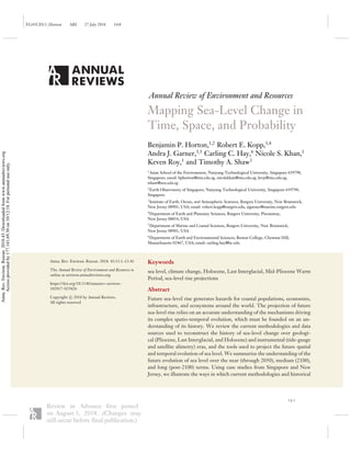
  • 13. EG43CH13_Horton ARI 27 July 2018 14:8 1.51.0 2.0 2.5 3.53.0 4.0 4.5 (n) Douglas (1997) (m) Holgate (2007) (l) Nerem et al. (2010) (e) Dangendorf et al. (2017) (g) Hay et al. (2015; KS) (f) Hay et al. (2015; GPR) (h) Jevrejeva et al. (2014) (j) Church & White (2011) (i) Ray & Douglas (2011) (k) Cazenave & Llovel (2010) (d) Jevrejeva et al. (2014) (c) Church et al. (2013) (b) Watson et al. (2015; VM1) (a) Watson et al. (2015; VM2) Satellite estimates (since 1993) Tide gauge reconstructions (20th and 21st century) 0.5 Sea-level rate (mm/year) Figure 4 Rates of sea-level rise, and the 1-σ uncertainty range, over the twentieth century (green dots) and over the satellite altimetry era (blue dots) derived from tide-gauge and satellite altimetry observations. The time windows for reach reconstruction are as follows: (a) 1993–2014 (VM2; 127) , (b) 1993–2014 (VM1; 127); (c) 1993–2010 (125); (d) 1993–2009 (117); (e) 1901–1990, 1993–2012 (118) ; ( f ) 1901–1990 (GPR; 119); (g) 1901–1990, 1993–2010 (KS; 119); (h) 1900–1999, 1993–2009 (117); (i) 1900–2009 (121) ; ( j) 1901–1990, 1993–2009 (116); (k) 1992–2010 (120) ; (l) 1993–2010 (26); (m) 1904–2003 (3); (n) 1880–1990 (207). Satellite altimetry: measurement of the height of the sea surface through satellite-based techniques such as radar altimetry They simulated local geoid changes and observations of vertical land motion to correct the tide gauges for local sea level effects, resulting in a 1901–1990 GMSL estimate of 1.1 ± 0.3 mm/year and a 1993–2012 estimate of 3.1 ± 1.4 mm/year. Tacklingtheproblemofspatio-temporalsparsitydifferently,Hayetal.(119)combinedthetide- gauge records with process-based models of the underlying physics driving global and regional sea-level change using two techniques: a multi-model Kalman smoother and Gaussian process regression. These two methodologies estimate GMSL by first estimating, from the tide-gauge record, the magnitudes of the individual processes contributing to local and global sea level, then summing the individual contributors to produce GMSL estimates. During 1901–1990, the Kalman smoother and Gaussian process regression techniques produced GMSL rise estimates of 1.2 ± 0.2 mm/year and 1.1 ± 0.4 mm/year, respectively. During the altimetry era, from 1993–2010, the Kalman smoother technique estimates that GMSL rose at 3.0 ± 0.7 mm/year (Figure 4). Since 1992, the long but incomplete tide-gauge record has been supplemented with near- global satellite altimetry observations. Satellite altimeter missions have provided maps of absolute sea level every 10 days within approximately ± 66o , permitting changes in the sea surface to be determined for the majority of the world ocean (120). Unlike tide gauges, which are inherently only located along the world’s coastlines, satellite altimetry observations have provided new insight into previously unobserved ocean basins. The combination of tide gauge and altimetry observations has the potential to shed new insights on both GMSL and RSL; however, combining these two data sources is also not a simple task. For example, coastal processes and vertical land motion, which are not observed by satellite altimeters, can be the dominant processes captured in tide-gauge records. Accurately characterizing and separating sea-level noise from sea-level signal is an ongoing challenge (116, 121). In empirical orthogonal function approaches, satellite altimetry observations are used to determine the dominant global patterns of sea surface height change over the past ∼25 years. The magnitudes of these patterns are then constrained over the twentieth century with the tide-gauge observations. GMSL estimates using this technique for 1901–1990 are www.annualreviews.org • Mapping Sea-Level Change in Time 13.13 Review in Advance first posted on August 3, 2018. (Changes may still occur before final publication.) Annu.Rev.Environ.Resour.2018.43.Downloadedfromwww.annualreviews.org Accessprovidedby177.141.69.30on10/12/18.Forpersonaluseonly.
  • 14. EG43CH13_Horton ARI 27 July 2018 14:8 approximately 1.5 ± 0.2 mm/year (116), whereas over the longer time period of 1900–2009, GMSL estimates increase to 1.7 ± 0.2 mm/year (Figure 4, 116, 121). It is a matter for debate as to whether the observed dominant short-term patterns of variability over the satellite era are the most appropriate ones to characterize patterns of long-term variability over the tide-gauge era (122). As the satellite altimetry record length grows, so does the satellite derived time series of (near) global mean sea surface height (123, 124). These estimates of 2.6–3.2 mm/year (125–127) are obtained by computing area weighted averages of the near global sea surface height fields. It is now possible to use the 25-year altimetry record to estimate the acceleration in GMSL since 1993. This acceleration of 0.084 ± 0.025 mm/year2 (128) represents a starting point for putting recent GMSL estimates into historical context. Developing new statistically robust methodologies to combine the satellite altimetry data with the tide gauge observations is an important and daunting task, and it is necessary in order to quantify local and regional accelerations over the twentieth century. 3.3. Attribution of Twentieth-Century Global Mean Sea-Level Change Attribution studies focus on the extent to which twentieth (and early twenty-first) century GMSL can be affirmatively tied to the effects of human-caused warming (129). These studies—relying on a variety of both physical modeling and statistical techniques—generally agree that a large portion of the twentieth-century rise, including most GMSL rise over the past quarter of the twentieth century, is tied to anthropogenic warming (25, 130–132). For example, Slangen et al. (132) used a suite of physical models of global climate and land-ice surface mass balance, together with correction terms for omitted factors, to compare GMSL with and without natural forcing. They found that natural forcing could account for approximately 50% of the modeled historical GMSL change from 1900–2005, and only approximately 10% of modeled historical GMSL change from 1970–2005. Kopp et al. (25) calibrated a statistical model to the relationship between temperature and rate of sea-level change over the past two millennia, and found that—had the twentieth-century global mean surface temperature been the same as the average over 500–1800 CE—twentieth-century GMSL rise would have been approximately 35% (90% probable range: −13 to +59%) of its instrumental value. 4. PROJECTIONS OF FUTURE SEA-LEVEL RISE Our knowledge of past and present changes in sea level can help us understand and predict its future evolution. Methods used to project sea-level changes in the future can be categorized along two basic axes: (1) the degree to which they disaggregate the different drivers of sea-level change, and (2) the extent to which they attempt to characterize probabilities of future outcomes (Figure 5). The former axis separates projections that tabulate individual processes—including projections focused on central ranges, scenarios attempting to assess upper bounds of plausible sea-level rise, and probabilistic bottom-up projections—from semi-empirical approaches based on global climate and sea-level statistics, as well as some expert judgement-based approaches. The latter axis separates approaches focused on assessing either central or extreme outcomes from fully probabilistic approaches. Sea-level rise projections published in the past several years have largely been conditional on different RCPs (133). The RCPs represent a range of possible future climate forcing path- ways, including a high-emission pathway with continued growth of CO2 emissions (RCP8.5), a moderate-emission pathway with stabilized emissions (RCP4.5), and a low-emission pathway con- sistent with the Paris Agreement’s goal (134) of net-zero CO2 emissions in the second half of this 13.14 Horton et al. Review in Advance first posted on August 3, 2018. (Changes may still occur before final publication.) Annu.Rev.Environ.Resour.2018.43.Downloadedfromwww.annualreviews.org Accessprovidedby177.141.69.30on10/12/18.Forpersonaluseonly.
  • 15. EG43CH13_Horton ARI 27 July 2018 14:8 Aggregated Disaggregated Disaggregation Distributioncomprehensiveness Point estimate Fully probabilistic Bottom-up scenarios Top-down scenarios Bottom-up central ranges High-end estimates Probabilistic approaches Semi-empirical models Top-down expert judgement Figure 5 Taxonomy of sea-level rise projections methods. The horizontal axis separates methods based on the degree to which they disaggregate the different drivers of sea-level change. The vertical axis separates methods based on the extent to which they attempt to characterize probabilities of future outcomes. Dynamic sea level: sea-surface height variations produced by oceanic and atmospheric circulation and by temperature and salinity distributions century (RCP2.6). The use of the RCPs enables comparisons among projections from different studies and different methods (135–142). 4.1. Bottom-Up Approaches Most projections are based on a bottom-up accounting of contributions from different driving factors of global and regional sea-level change. Estimates of different contributing factors may be based on a quantitative or semi-quantitative literature meta-analysis. For example, climate models such as those included in the Coupled Model Intercomparison Projection Phase 5 are often used to inform projections of thermal expansion and dynamic sea-level change as well as to drive models of glacier surface mass balance. Alternatively, estimates of factors that contribute to sea-level rise may also be based on the output of a single model study of complex processes such as marine–ice sheet dynamics [e.g., the use of DeConto & Pollard (143) in Kopp et al. (144)] or on simplified models that capture the core dynamics of a process such as ocean heat uptake in response to climate forcing (135, 142). Estimates of sea-level contributions may also be based on heuristic judgements, for example, of the plausible acceleration of ice flow through outlet glaciers (145). 4.1.1. Central-range estimates. In the literature, many bottom-up estimates focus on charac- terizing central ranges for key contributing factors, defined by a median, a single low quantile, and a single high quantile (e.g., 146, 147), typically the 17th and 83rd or 5th and 95th percentile values. 4.1.2. High-end estimates. High-end (sometimes referred to as “worst-case”) bottom-up es- timates complement central-range estimates. Pfeffer et al. (145) constructed a high-end (2.0 m GMSL rise by 2100) sea-level rise scenario based on plausible accelerations of Greenland ice discharge, determined partially by the fastest local, annual rates of ice-sheet discharge currently www.annualreviews.org • Mapping Sea-Level Change in Time 13.15 Review in Advance first posted on August 3, 2018. (Changes may still occur before final publication.) Annu.Rev.Environ.Resour.2018.43.Downloadedfromwww.annualreviews.org Accessprovidedby177.141.69.30on10/12/18.Forpersonaluseonly.
  • 16. EG43CH13_Horton ARI 27 July 2018 14:8 observed. This estimate has subsequently been debated, and additional contributions from thermal expansion [based on an Earth system model (148)], groundwater discharge, and Antarctica (e.g., 55) have been suggested, raising the high-end projection to ∼2.6 m. Furthermore, the highest among DeConto & Pollard’s (143) ensemble of Antarctic simulations exceeded 1.7 m of sea-level rise from Antarctica alone in 2100 under RCP8.5, suggesting that high-end outcomes well in excess of 3 m of GMSL rise by 2100 cannot be excluded under RCP8.5. 4.1.3. Probabilistic approaches. Probabilistic approaches build on both the central range and high-end approaches, aiming to estimate a single, comprehensive probability distribution of sea- level rise from a bottom-up accounting of different components. The relationship between central range projections and probabilistic projections can be relatively straightforward: central range projections are often presented with 1 or 2σ putative standard errors (e.g., 147), which have a natural probabilistic interpretation if a particular distributional form is assumed. The relationship between high-end estimates and probabilistic projections is interpreted in a broader variety of ways. For example, Kopp et al. (140) highlighted the agreement between the 99.9th percentile of their RCP8.5 GMSL projection (2.5 m) and other high-end estimates, whereas Jevrejeva et al. (126) used the 95th percentile of an RCP8.5 projection (1.8 m) as an upper limit. The first published probabilistic GMSL projections were developed by Titus & Narayanan (149) for the US Environmental Protection Agency, based on a suite of coupled simple physical models with parameters informed by structured expert elicitation. Probabilistic approaches expe- rienced a resurgence in the past half-decade, in part because of concerns regarding the adequacy of communication about high-end uncertainty in IPCC AR5 sea-level projections (126, 137, 138, 140). Probabilistic studies have been largely constrained to use the climate scenarios run by large model intercomparison projects. However, some more recent probabilistic studies rely on simple coupled models of different components, allowing for more flexible simulations (135, 136, 141, 142, 150). 4.2. Top-Down Approaches Top-down approaches for estimating GMSL focus on comprehensive metrics of change, rather than a bottom-up accounting of individual driving factors. Most top-down studies are semi- empirical in nature. 4.2.1. Semi-empirical approaches. Semi-empirical approaches rely on historical statistical re- lationships between GMSL change and driving factors such as temperature. One of the earliest GMSL projections (151) used such a relationship, fitting approximated GMSL as a lagged linear function of global mean surface temperature; their relationship (roughly 16 cm/◦ C) would yield a likely twenty-first century GMSL rise of approximately 0.2–0.3 m under RCP2.6, and 0.4–0.8 m under RCP8.5. They noted, however, the potential for rapid loss of marine-based ice in Antarctica to raise their projections significantly. This particular study did not formally account for uncer- tainty in the relationship between temperature and sea level, and thus would fall at the lower end of our probabilistic axis. However, uncertainty analysis is straightforward with simple parametric approaches, and subsequent semi-empirical studies have generally been highly probabilistic. The current generation of semi-empirical approaches began with Rahmstorf (152), who fit the historical rate of GMSL change as a function of temperature disequilibrium. Combining a semi-empirical approach that includes uncertainty estimates on key parameters with probabilistic projections of the global mean surface temperature response to different forcing scenarios can yield formally complete probability distributions of future GMSL rise. Such projections are, however, 13.16 Horton et al. Review in Advance first posted on August 3, 2018. (Changes may still occur before final publication.) Annu.Rev.Environ.Resour.2018.43.Downloadedfromwww.annualreviews.org Accessprovidedby177.141.69.30on10/12/18.Forpersonaluseonly.
  • 17. EG43CH13_Horton ARI 27 July 2018 14:8 sensitive to the choice of calibration data set—an additional level of uncertainty not typically formally quantified within a single study and preventing a formal probabilistic evaluation. These choices can have a significant impact. For example, Kopp et al. (144), using a calibration based on reconstructions of temperature and GMSL over the past two millennia, project a rise of 0.3–0.9 m (at the 90% confidence level) over the twenty-first century under RCP4.5, whereas Schaeffer et al. (153), using a calibration based on a single geological reconstruction from North Carolina (5), project 0.6–1.2 m. 4.2.2. Expert judgement. In the course of scientific practice, experts integrate many streams of information to revise their assessments of the world and the way it behaves; Bayes’ theorem, as used in formal statistical analyses, is a formalization of this process. On some level, all projections of future change are based on expert judgement, frequently expressed within the deliberative context of a scientific publication or assessment panel. A variety of approaches—some relatively informal, others based on more rigorous social scien- tific practices—use this integration process executed by individuals as an object of study in its own right, and extract from it estimates of the likelihood of different future outcomes. In the sea-level realm, structured expert elicitation—a formal method in which experts are guided in the inter- pretation of probabilities in a workshop setting before having their responses weighted based on their performance on calibration questions—has been used to assess the probability distribution of future ice-sheet changes (154). Less structured, more informal expert surveys have also been used to assess the response of GMSL as a whole to different forcing scenarios (155). 4.3. Methods of Using Sea-Level Rise Projections The approaches described above are “science-first” approaches—focused on integrating a variety of lines of information to produce a scientific judgement about future global and/or regional sea- level changes. These approaches are not generally designed to produce projections that can be directly used in a decision process. Yet in the absence of ongoing dialogue between scientists and decision makers, this distinction can give rise to confusion. For example, approaches focused ex- clusively on central ranges omit information about high-end outcomes that can be crucial for risk management, whereas approaches focused exclusively on high-end estimates could lead to exces- sively costly and conservative decisions. Bottom-up probabilistic approaches and semi-empirical approaches can provide self-consistent information about both central tendencies and high-end outcomes, but relying on results from a single estimated probability distribution can mask ambi- guity and potentially provide a false sense of security about the (un)likelihood of extreme outcomes (156). Caveats expressed in primary scientific literature are frequently lost in the translation to assessment reports. 4.3.1. Scenario approaches. One approach to dealing with these challenges is to use the un- derlying scientific literature—drawing on multiple methodologies—to develop scenarios against which decisions can be tested. For example, the National Research Council defined a range of heuristically motivated “plausible variations in GMSL rise,” spanning 50–150 cm between the 1980s and 2100, which they recommended be used for engineering sensitivity analyses (157). In some contexts, such scenario-based projections are categorized together with scientific projec- tions. We argue that this is a categorization error: Discrete scenarios for decision analysis can be scientifically justified only when based on projections developed using the suite of scientific approaches discussed above. www.annualreviews.org • Mapping Sea-Level Change in Time 13.17 Review in Advance first posted on August 3, 2018. (Changes may still occur before final publication.) Annu.Rev.Environ.Resour.2018.43.Downloadedfromwww.annualreviews.org Accessprovidedby177.141.69.30on10/12/18.Forpersonaluseonly.
  • 18. EG43CH13_Horton ARI 27 July 2018 14:8 Deep uncertainty: also known as ambiguity or Knightian uncertainty; describes uncertainties for which it is not possible to develop a single, well-characterized probability distribution 4.3.2. Probabilistic approaches and deep uncertainty. One motivation for developing com- plete probability distributions for future sea-level rise is their direct utility in specific decision frameworks. For example, benefit-cost analyses employ probability distributions of future change as an input; probabilistic projections are thus crucial for assessing metrics such as the social cost of greenhouse gas emissions (e.g., 158). Similarly, probability distributions of future sea-level rise can be combined with probability distributions of future storm tides to estimate future flood prob- abilities (e.g., 159, 160). However, some decision makers have expressed confusion regarding the distinction between Bayesian probabilities of future changes and historical, frequentist probability distributions for variables such as storm tides in a stationary climate. Although the reality of climate change means that no probability distribution can be truly based on the assumption of station- arity, the familiarity of such assumptions can mask deep uncertainty and lead to overconfidence (156). Sea-level rise projections, particularly for the second half of this century and beyond, exhibit ambiguity: They have no uniquely specifiable probability distribution, and different approaches yield distributions that differ considerably. The field of decision making under uncertainty has developed several approaches to cope with ambiguity (e.g., 161). Some approaches rely on em- ploying multiple probability distributions, which can reveal the robustness (or lack thereof ) of a probability-based judgement to the underlying uncertainty in scientific knowledge that may not be captured within a single probability distribution. Possibility theory (162) provides one approach for combining multiple lines of evidence to produce a “probability box” that bounds the upper and lower limits of different quantiles of a probability distribution, revealing areas of relatively low and relatively high ambiguity. We apply a simpler but related approach below, summarizing literature projections for different scenarios in “very likely” ranges that are constructed from the minima of 5th-percentile projections and maxima of 95th-percentile projections. 4.4. Sea-Level Rise Projections We summarize recent literature projections of GMSL rise for 2050, 2100, 2150, and 2300, as well as recent studies on multi-millennial sea-level rise commitments (Table 1, Figure 6a). Most of these studies are based on the RCPs, which allow the quantile projections produced by different studies to be directly compared to one another. Sea-level rise projections conditional on different RCPs do not, however, align with the differ- ent temperature targets laid out in the 2015 Paris Agreement, which aims to hold “the increase in the global average temperature to well below 2◦ C above pre-industrial levels and [pursue] efforts to limit the temperature increase to 1.5◦ C above pre-industrial levels” (134, §2-1a). Among the RCPs, both the 2.0◦ C and 1.5◦ C Paris Agreement temperature targets are most consistent with RCP2.6, although some RCP4.5 projections are consistent with 2.0◦ C. Thus, there has also been a recent set of studies focused on different scenarios consistent with these goals, providing another point for cross-study comparison (163–166). In order to compare values across different studies that use different temporal baselines, we have normalized sea-level projections: SLRAd j = SLR t (Y − Y0) , 1. where SLRAd j is the normalized sea-level rise projection, SLR is the sea-level rise reported in the study, t is the time range in years (in the case of 2050 projections, t = 50), Y is the study end year, and Y0 is the study baseline year. In cases where a range of years is used for either the study endpoint, or for the study baseline, we use the central year from the range for Equation 1 above. 13.18 Horton et al. Review in Advance first posted on August 3, 2018. (Changes may still occur before final publication.) Annu.Rev.Environ.Resour.2018.43.Downloadedfromwww.annualreviews.org Accessprovidedby177.141.69.30on10/12/18.Forpersonaluseonly.
  • 19. EG43CH13_Horton ARI 27 July 2018 14:8 Table 1 Global mean sea-level rise projections (median, 17th to 83rd percentile range, and 5th to 95th percentile range)a Year Percentile range projections 50 (median) 17–83 5–95 Probabilistic projections Kopp14 RCP8.5 2050 0.29 0.24–0.34 0.21–0.38 2100 0.79 0.62–1.00 0.52–1.21 2150 1.30 1.00–1.80 0.80–2.30 2300 3.18 1.75–5.16 0.98–7.37 RCP4.5 2050 0.26 0.21–0.31 0.18–0.35 2100 0.59 0.45–0.77 0.36–0.93 2150 0.90 0.60–1.30 0.40–1.70 2300 1.92 0.7–3.49 0–5.31 RCP2.6 2050 0.25 0.21–0.29 0.18–0.33 2100 0.50 0.37–0.65 0.29–0.82 2150 0.70 0.50–1.10 0.30–1.50 2300 1.42 0.32–2.88 −0.22–4.70 Grinsted15 RCP8.5 2100 0.80 0.58–1.20 0.45–1.83 Jackson16 RCP8.5 High-end 2050 0.27 0.20–0.34 0.17–0.44 2100 0.80 0.60–1.16 0.49–1.60 RCP8.5 2100 0.72 0.52–0.94 0.35–1.13 RCP4.5 2100 0.52 0.34–0.69 0.21–0.81 Kopp17 RCP8.5 2050 0.31 0.22–0.40 0.17–0.48 2100 1.46 1.09–2.09 0.83–2.43 2150 4.09 3.17–5.47 2.92–5.98 2300 11.69 9.80–14.09 9.13–15.52 RCP4.5 2050 0.26 0.18–0.36 0.14–0.43 2100 0.91 0.66–1.25 0.50–1.58 2150 1.72 1.21–2.72 0.90–3.22 2300 4.21 2.75–5.95 2.11–6.96 (Continued) www.annualreviews.org • Mapping Sea-Level Change in Time 13.19 Review in Advance first posted on August 3, 2018. (Changes may still occur before final publication.) Annu.Rev.Environ.Resour.2018.43.Downloadedfromwww.annualreviews.org Accessprovidedby177.141.69.30on10/12/18.Forpersonaluseonly.
  • 20. EG43CH13_Horton ARI 27 July 2018 14:8 Table 1 (Continued) Year Percentile range projections 50 (median) 17–83 5–95 RCP2.6 2050 0.23 0.16–0.33 0.12–0.41 2100 0.56 0.37–0.78 0.26–0.98 2150 0.87 0.55–1.21 0.39–1.52 2300 1.42 0.83–2.30 0.50–3.00 Nauels17a RCP8.5 2050 0.25 0.20–0.30 2100 0.71 0.58–0.87 2150 3.76 2.74–5.25 2300 4.66 3.36–6.72 RCP4.5 2050 0.23 0.19–0.28 2100 0.52 0.43–0.63 2150 1.21 0.70–1.56 2300 1.73 1.27–2.27 RCP2.6 2050 0.22 0.17–0.27 2100 0.43 0.34–0.54 2150 0.63 0.50–0.83 2300 1.00 0.79–1.33 Jackson18 Stab2.0 2100 0.48 0.33–0.61 0.23–0.71 Stab1.5 2100 0.42 0.29–0.56 0.19–0.64 Rasmussen18 Stab2.0 2050 0.25 0.20–0.32 0.17–0.37 2100 0.55 0.40–0.75 0.30–0.94 2150 0.89 0.54–1.34 0.35–1.78 Stab1.5 2050 0.24 0.20–0.28 0.18–0.32 2100 0.47 0.35–0.64 0.28–0.82 2150 0.68 0.41–1.06 0.28–1.50 Semi-empirical projections Jevrejeva12 RCP8.5 2050 0.33 0.24–0.46 2100 1.00 0.74–1.50 (Continued) 13.20 Horton et al. Review in Advance first posted on August 3, 2018. (Changes may still occur before final publication.) Annu.Rev.Environ.Resour.2018.43.Downloadedfromwww.annualreviews.org Accessprovidedby177.141.69.30on10/12/18.Forpersonaluseonly.
  • 21. EG43CH13_Horton ARI 27 July 2018 14:8 Table 1 (Continued) Year Percentile range projections 50 (median) 17–83 5–95 RCP4.5 2050 0.29 0.21–0.41 2100 0.67 0.47–1.00 RCP3-PD 2050 0.27 0.20–0.38 2100 0.52 0.33–0.75 Schaeffer12 RCP8.5 2100 1.02 0.72–1.39 RCP4.5 2100 0.90 0.64–1.21 2300 3.55 2.12–5.27 RCP3-PD 2100 0.75 0.52–0.96 2300 1.99 1.18–3.09 Stab2.0 2100 0.80 0.56–1.05 2300 2.67 1.56–4.01 Stab1.5 2100 0.77 0.54–0.99 2300 1.49 0.87–2.36 Kopp16 RCP8.5 2100 0.76 0.59–1.05 0.52–1.31 RCP4.5 2100 0.51 0.39–0.69 0.33–0.85 RCP2.6 2100 0.38 0.28–0.51 0.24–0.61 Bittermann17 Stab2.0 2050 0.24 0.19–0.31 2100 0.50 0.39–0.61 2150 0.67 0.50–0.86 Stab1.5 2050 0.19 0.15–0.24 2100 0.37 0.29–0.46 2150 0.49 0.36–0.65 Jackson18 Stab2.0 2100 0.65 0.45–0.89 0.31–1.12 Stab1.5 2100 0.55 0.38–0.74 0.27–0.89 (Continued) www.annualreviews.org • Mapping Sea-Level Change in Time 13.21 Review in Advance first posted on August 3, 2018. (Changes may still occur before final publication.) Annu.Rev.Environ.Resour.2018.43.Downloadedfromwww.annualreviews.org Accessprovidedby177.141.69.30on10/12/18.Forpersonaluseonly.
  • 22. EG43CH13_Horton ARI 27 July 2018 14:8 Table 1 (Continued) Year Percentile range projections 50 (median) 17–83 5–95 Central range Perrette13 RCP8.5 2050 0.28 0.23–0.34 2100 1.06 0.78–1.43 RCP4.5 2050 0.28 0.23–0.32 2100 0.86 0.66–1.11 RCP3-PD 2050 0.28 0.23–0.32 2100 0.75 0.49–0.94 Slangen14 RCP8.5 2100 0.74 0.45–1.04 RCP4.5 2100 0.57 0.37–0.77 Mengel16 RCP8.5 2050 0.19 0.14–0.26 2100 0.81 0.55–1.26 RCP4.5 2050 0.17 0.13–0.22 2100 0.51 0.35–0.74 RCP2.6 2050 0.17 0.12–0.21 2100 0.38 0.27–0.53 Schleussner16 Stab2.0 2100 0.50 0.36–0.65 Stab1.5 2100 0.41 0.29–0.53 Bakker17 RCP8.5 2050 0.23 0.21–0.34 2100 1.11 0.81–1.52 RCP4.5 2050 0.21 0.19–0.31 2100 0.68 0.52–0.93 (Continued) 13.22 Horton et al. Review in Advance first posted on August 3, 2018. (Changes may still occur before final publication.) Annu.Rev.Environ.Resour.2018.43.Downloadedfromwww.annualreviews.org Accessprovidedby177.141.69.30on10/12/18.Forpersonaluseonly.
  • 23. EG43CH13_Horton ARI 27 July 2018 14:8 Table 1 (Continued) Year Percentile range projections 50 (median) 17–83 5–95 RCP2.6 2050 0.18 0.17–0.29 2100 0.51 0.38–0.68 Goodwin17 RCP8.5 2100 0.73–1.05 RCP4.5 2100 0.53–0.86 RCP2.6 2100 0.43–0.67 Nauels17b RCP8.5 2050 0.25 0.18–0.33 2100 0.88 0.59–1.27 RCP4.5 2100 0.67 0.43–0.99 RCP2.6 2050 0.20 0.14–0.29 2100 0.49 0.33–0.71 Wong17 RCP8.5 2050 0.30 0.25–0.40 2100 1.50 1.09–2.07 RCP4.5 2050 0.28 0.22–0.35 2100 0.77 0.56–1.30 RCP2.6 2050 0.26 0.20–0.33 2100 0.55 0.43–0.74 a Studies have been categorized as probabilistic (projections that sample uncertainty for different driving factors and present multiple quantiles in the original study), semi-empirical (projections made with a model that uses a statistical relationship between global mean temperature and GMSL, without computing individual factors), or central range (projections that are either not semiempirical and also do not sample uncertainty for different driving factors, or that focus the original study exclusively on a central, low, and high quantile). b Probabilistic models include Kopp14 (140), Grinsted15 (137), Jackson16 (138), Kopp17 (144), Nauels17a (142), Jackson18 (164), and Rasmussen18 (165). Semi-empirical models include Jevrejeva12 (139), Schaeffer12 (153), Kopp16 (25), Bittermann17 (163), and Jackson18 (164). Central range models include Perrette13 (208), Slangen14 (147), Mengel16 (141), Schleussner16 (166), Bakker17 (135), Goodwin17 (136), Nauels17b (209), and Wong17 (150). www.annualreviews.org • Mapping Sea-Level Change in Time 13.23 Review in Advance first posted on August 3, 2018. (Changes may still occur before final publication.) Annu.Rev.Environ.Resour.2018.43.Downloadedfromwww.annualreviews.org Accessprovidedby177.141.69.30on10/12/18.Forpersonaluseonly.
  • 24. EG43CH13_Horton ARI 27 July 2018 14:8 4.4.1. Projections for 2050. Near-term projections (through 2050) exhibit minimal sensitivity to emission pathways and a relatively small spread among studies (135, 138–141, 144, 150, 163). Across various RCPs and temperature scenarios, median GMSL projections in these studies range from 0.2–0.3 m. A conservative interpretation of these different studies would place the very likely GMSL rise between 2000 and 2050, across possible forcing pathways, at 0.1–0.5 m, with the benefit of transitioning from rapid emission growth to rapid emission decline being <0.1 m (Table 1, Figure 6a). 4.4.2. Projections for 2100. In the second half of the century and beyond, the spread in pro- jections grows substantially due to both alternative methods and emissions uncertainty. Within a 0 0.1 0.2 0.3 0.4 0.5 Rasmussen18 Jackson18 SE Jackson18 PB Bittermann17 Schleussner16 Schaeffer12 Rasmussen18 Jackson18 SE Jackson18 PB Bittermann17 Schleussner16 Schaeffer12 Wong17 Nauels17b Nauels17a Kopp17 DP16 Goodwin17 sToSL Bakker17 Mengel16 Kopp16 Jackson16 Jackson16 HighEnd Grinsted15 Slangen14 Kopp14 Perrette13 Schaeffer12 Jevrejeva12 Wong17 Nauels17b Nauels17a Kopp17 DP16 Goodwin17 sToSL Bakker17 Mengel16 Kopp16 Jackson16 Slangen14 Kopp14 Perrette13 Schaeffer12 Jevrejeva12 Wong17 Nauels17b Nauels17a Kopp17 DP16 Goodwin17 sToSL Bakker17 Mengel16 Kopp16 Kopp14 Perrette13 Schaeffer12 Jevrejeva12 Sea-level rise (m) 2050 0 0.5 1 1.5 2 2.5 2100 Figure 6 (a) Near-term (2050; left), mid-term (2100; center), and long-term (2300; right) sea-level rise projections for RCP2.6, RCP4.5, and RCP8.5 scenarios, respectively, as well as for scenarios stabilizing global mean temperature at 1.5◦C (Stab1.5) and 2.0◦C (Stab2.0) above preindustrial levels (Stab1.5). Shown are the 5-95th-percentile ranges (thin bars), 17th–83rd percentile ranges (thick bars), and median (circles) global mean sea-level (GMSL) rise projections (in meters). The AR5 “likely” ranges of 2050 and 2100 sea-level rise for each RCP scenario are shown by colored shading on the left and center panels, respectively. Gray shading on the right-most panel represents the range of IPCC AR5 2300 sea-level rise projections. (b) Decomposition of uncertainty in GMSL projections, following the DP16 projections of Kopp et al. (144). Red represents within-scenario variance due to the Antarctic ice sheet (AIS), cyan the variance due to the Greenland ice sheet (GIS), blue the variance due to glaciers and ice caps (GIC), green the variance due to thermal expansion (TE), and purple the variance due to land-water storage (LWS). The yellow line represents the total variance, pooling across RCP2.6, RCP4.5, and RCP8.5 (Scen). Until the 2040s, cross-scenario variance is negligible, leading to a total variance across RCPs that is slightly smaller than the variance within RCP4.5 (represented by the sum of all other contributions). In the second half of the twenty-first century, across-scenario variance grows to dominate uncertainty. 13.24 Horton et al. Review in Advance first posted on August 3, 2018. (Changes may still occur before final publication.) Annu.Rev.Environ.Resour.2018.43.Downloadedfromwww.annualreviews.org Accessprovidedby177.141.69.30on10/12/18.Forpersonaluseonly.
  • 25. EG43CH13_Horton ARI 27 July 2018 14:8 0 0.2 0.4 0.6 0.8 1 Fractionofvariance 2020 2040 2060 2080 2100 Year (CE) Scen LWS TE GIC GIS AIS b 0 2 4 6 8 10 12 14 16 2300 RCP2.6RCP2.6RCP2.6 RCP4.5RCP4.5RCP4.5 RCP8.5RCP8.5RCP8.5 Stab1.5Stab1.5Stab1.5 Stab2.0Stab2.0Stab2.0 Sea-level rise (m) Figure 6 (Continued) a single forcing pathway, uncertainty in the response of the polar ice sheets to climate changes becomes increasingly dominant (Figure 6b), but uncertainty across scenarios becomes at least as large and often larger. Across RCPs and studies, median projections for total twenty-first-century GMSL rise range from as low as 0.4 m under RCP2.6 (25, 141) to as high as 1.5 m under RCP8.5 in simulations allowing for an aggressively unstable Antarctic ice sheet (150). Scenario choice exerts a great deal of influence, with median projections ranging from 0.4 to 0.8 m under RCP2.6, 0.5 to 0.9 m under RCP4.5, and 0.7 to 1.5 m under RCP8.5 (25, 135–142, 144, 147, 150). Assessing across studies yields a very likely GMSL rise of 0.2–1.0 m under RCP2.6, 0.2–1.6 m under RCP4.5, and 0.4–2.4 m under RCP8.5 (Table 1, Figure 6a). Studies attempting to assess the difference in GMSL rise between 1.5◦ C and 2.0◦ C warmer worlds that are consistent with goals of the Paris Agreement largely occupy the space of RCP2.6 and the cooler fraction of RCP4.5 projections. Excluding one older semi-empirical study (153), normalized projections of median 2100 sea-level rise range from 0.4–0.6 m under a scenario in which global average temperatures stabilize at 1.5◦ C (163) and from 0.5–0.7 m under a scenario in which global average temperatures stabilize at 2.0◦ C (164). Across studies, very likely ranges are 0.2–1.0 m under 1.5◦ C stabilization and 0.2–1.1 m under 2.0◦ C stabilization (163–166). 4.4.3. Projections for 2150. Across the past three and a half decades, the end of the twenty- first-century has remained the endpoint of most GMSL projections, even as that endpoint has crept closer. With the twenty-second century now within the lifetime of some infrastructure www.annualreviews.org • Mapping Sea-Level Change in Time 13.25 Review in Advance first posted on August 3, 2018. (Changes may still occur before final publication.) Annu.Rev.Environ.Resour.2018.43.Downloadedfromwww.annualreviews.org Accessprovidedby177.141.69.30on10/12/18.Forpersonaluseonly.
  • 26. EG43CH13_Horton ARI 27 July 2018 14:8 Marine Isotope Stages: warm and cool periods in Earth paleoclimate inferred from oxygen isotope data from deep sea core samples; timescale was developed by Cesare Emiliani in the 1950s as a standard to correlate Quaternary climate records investments, a small number of studies have looked beyond (140, 142, 144). Across three studies, median estimates of GMSL rise between 2000 and 2150 range from 0.6–0.9 m under RCP2.6, 0.9–1.7 m under RCP4.5, and 1.3–4.1 m under RCP8.5. Across studies, very likely ranges are 0.3–1.5 m under RCP2.6, 0.4–3.2 m under RCP4.5, and 0.8–6.0 m under RCP8.5. Among studies focused on the difference between 1.5◦ C and 2.0◦ C of warming, two (163, 165) have projected 2150 sea-level rise. Median projections extend from 0.5 m to 0.7 m for 1.5◦ C of warming and from 0.7 m to 0.9 m for 2.0◦ C of warming. Very likely ranges are 0.3–1.5 m for 1.5◦ C and 0.4–1.8 m for 2.0◦ C. 4.4.4. Projections for 2300. The same three studies providing 2150 RCP projections (140, 142, 144) also provide projections through 2300, the temporal endpoint of the extensions of the RCPs.1 One semi-empirical study (167) also provides projections on this timescale. Unsurprisingly, the difference among scenarios is extremely large by 2300—by which time, the extension of RCP2.6 is characterized by an atmospheric CO2 concentration lower than today, whereas the extension of RCP8.5 is characterized by a CO2 concentration of nearly 2,000 ppm. Median estimates of GMSL rise between 2000 and 2300 range from 1.0–2.0 m under RCP2.6, 1.7–4.2 m under RCP4.5, and 3.2–11.7 m under RCP8.5. Across studies, very likely ranges are −0.2 to 4.7 m under RCP2.6, 0.0 to 7.0 m under RCP4.5, and 1.0 to 15.5 m under RCP8.5 (Figure 6a). Kopp et al. (144) provide two sets of projections, one (labeled K14), based on an extension of Kopp et al. (140) that, for ice sheets, is largely consistent with the IPCC’s Fifth Assessment Report, and one (labeled DP16) incorporating results from the Antarctic ice-sheet model of DeConto & Pollard (143). The difference between these two projections highlights the importance of Antarctic ice-sheet behavior on this timescale. In K14, the 90% credible projections are −0.2 to 4.7 m under RCP2.6, 0.0 to 5.3 m under RCP4.5, and 1.0 to 7.4 m under RCP8.5. In DP16, the corresponding projections are 0.5–3.0 m under RCP2.6, 2.1–7.0 m under RCP4.5, and 9.1–15.6 m under RCP8.5. The incorporation of the results of a mechanistic model for the Antarctic ice sheet narrows the projection range under low emissions but shifts and fattens it under high emissions. 4.4.5. Multi-millennial projections. The effects of climate change on sea level are not felt instantaneously; rather, due to the slow response time of deep ocean heat uptake and the sluggish response of ice sheets, they play out over millennia. The long-term sea-level response to a given emission future is sometimes called a “sea-level commitment” (168). Levermann et al. (168) use a combination of physical models for ocean warming, glaciers, ice caps, and ice-sheet contributions to assess the sea-level change arising from two millennia of exposure to a constant temperature. Over 2,000 years, they find a sea-level commitment of approximately 2.3 m/◦ C of warming. They note, however, that over longer time periods Greenland exhibits an abrupt threshold of ice loss between 0.8 and 2.2◦ C that ultimately adds approximately 6 m to GMSL. Incorporating this abrupt threshold yields a relationship, they conclude, that is consistent with paleo–sea-level constraints from the LIG, the MPWP, and Marine Isotope Stage 11 (approximately 411–401 thousand years ago). Over two millennia, they project a commitment of 1.4–5.2 m from 1◦ C of warming, 3.0– 7.7 m from 2◦ C of warming, and 6.0–12.1 m from 4◦ C of warming. Over ten millennia, these numbers increase to 1.5–10.9 m, 3.5–13.5 m, and 12.0–16.0 m. Clark et al. (169) use physical models to consider not only the translation between temperature and long-term sea-level change, but also the translation between emissions and temperature. For a scenario in which 1,280 Gt C are emitted after the year 2000—roughly comparable to RCP4.5, and leading to a peak warming 1 Kopp et al.’s (140) projections are extended to 2300 in Kopp et al. (144). 13.26 Horton et al. Review in Advance first posted on August 3, 2018. (Changes may still occur before final publication.) Annu.Rev.Environ.Resour.2018.43.Downloadedfromwww.annualreviews.org Accessprovidedby177.141.69.30on10/12/18.Forpersonaluseonly.
  • 27. EG43CH13_Horton ARI 27 July 2018 14:8 of approximately 2.5◦ C above preindustrial levels—they find a 10,000-year sea-level commitment in excess of 20 m. They estimate that historical CO2 emissions have already locked in 1.2–2.2 m of sea-level rise, and phasing emissions down to zero over the course of the next ∼90 years will lock in another ∼9 m. A few additional studies have focused on individual drivers of sea-level rise and the possible long-term contributions to sea level from specific mechanisms. Numerous studies have used Earth system models of intermediate complexity to assess the long-term thermal expansion contribution to GMSL rise, which amounts to approximately 0.2–0.6 m/◦ C (11). Zickfeld et al. (170) found that the slow response time of the oceans is important even for their response to short-lived climate forcers. For example, if CH4 emissions cease, 75% of the CH4-induced thermal expansion persists for 100 years, and approximately 40% persists for 500 years. In addition, other studies have used coupled ice-sheet/ice-shelf models to examine the long- term response of the Antarctic ice sheet to RCP forcings. Golledge et al. (171) found that RCP2.6 would lead to 0.1–0.2 m of GMSL rise from Antarctica by 2300 and 0.4–0.6 m by 5000 CE, whereas RCP4.5 would lead to 0.6–1.0 m by 2300 and 2.8–4.3 m by 5000 CE, and RCP8.5 would lead to 1.6–3.0 m by 2300 and 5.2–9.3 m by 5000 CE. DeConto & Pollard (143), using an ice- sheet model that accounts for marine ice-sheet instability, ice-shelf hydrofracturing, and ice-cliff collapse, found that RCP2.6 would lead to approximately −0.5 to +2.4 m of GMSL rise from Antarctica by 2500 CE, whereas RCP4.5 would lead to 2.0–7.1 m and RCP8.5 to 9.7–17.6 m. 5. SYNTHESIS Bayesian and related probabilistic approaches are becoming increasingly widespread in recon- structing the spatio-temporal history of GMSL and RSL (e.g., 12, 25, 119). Bayesian reasoning represents a formal, probabilistic extension of the method of multiple working hypotheses, in- volving the identification of either a discrete or continuous set of alternative hypotheses or an assessment of the strength of prior evidence for each hypothesis. To date, however, probabilistic analyses of past and future changes have largely transpired in different domains. One of the ad- vantages of the rigor provided by formal approaches is that this need not be the case. Uncertainty quantification in future projections can guide the identification of useful research questions for paleo–sea level science, and the resulting improvements in understanding the past can lead to refined future projections. Probabilistic projections allow the identification of the major drivers of variance and, thus, the areas where investigation has the potential to yield the greatest reduction in that variance. Under the DP16 projections of Kopp et al. (144), for example, RSL projections in New Jersey (Figure 7) and Singapore (Figure 8) both are highly sensitive to the fate of the Antarctic ice sheet. Physical uncertainty in the Antarctic response (distinct from scenario uncertainty) accounts for at least ∼25% of projection variance at both sites throughout the twenty-first century. In Singapore, the second largest contributor to projection variance for much of the century is the geological back- ground (e.g., land subsidence), and the third largest contributor is atmosphere/ocean dynamics. By contrast, in New Jersey, atmosphere/ocean dynamics are the dominant contributor to variance through most of the century, whereas uncertainty in the geological background is negligible. This analysis would, thus, guide research to improve RSL projections in both localities toward the Antarctic, but it also highlights the importance of the geological background in Singapore and of a better characterization of North Atlantic atmosphere/ocean dynamics (Figures 7 and 8). The deep uncertainty regarding the behavior of marine-based parts of the Antarctic ice sheet has been noted since the earliest days of modern GMSL rise projections (e.g., 151), based on ge- ological considerations. The Antarctic response during past warm periods serves as an important www.annualreviews.org • Mapping Sea-Level Change in Time 13.27 Review in Advance first posted on August 3, 2018. (Changes may still occur before final publication.) Annu.Rev.Environ.Resour.2018.43.Downloadedfromwww.annualreviews.org Accessprovidedby177.141.69.30on10/12/18.Forpersonaluseonly.
  • 28. EG43CH13_Horton ARI 27 July 2018 14:8 0 1 2 3 RSL(m) RCP8.5 RCP4.5 RCP2.6 2000 2010 2020 2030 2040 2050 2060 2070 2080 2090 2100 Year (CE) 0 0.5 1 Fractionofvariance Scen Geo DSL LWS TE GIC GIS AIS –3000 –2500 –2000 –1500 –1000 –500 0 500 1000 1500 2000 Year (CE) –12 –10 –8 –6 –4 –2 0 RSL(m) a Atlantic City, New Jersey b c Figure 7 (a) Geological reconstruction of past relative sea level (RSL) in Atlantic City, New Jersey. Red boxes indicate sea-level index points within 0.5◦ angular distance. The yellow-orange curve indicates annual tide-gauge data. The gray curve is a prediction of past RSL at Atlantic City from a spatio-temporal empirical hierarchical model (25) fit to a database of western North Atlantic sea-level proxies and tide-gauge data. (b) Projections of RSL change in Atlantic City, New Jersey, under the RCP2.6 (green), RCP4.5 (orange), and RCP8.5 (purple) emission scenarios, from the DP16 projections of Kopp et al. (144). Lines indicate median projections; boxes indicate 5th–95th percentile projections for 2100, relative to 2000 CE. (c) Drivers of the uncertainty in the RSL projections of b. Wedges indicate the fractional contributions of different processes to the total variance, pooled across the three RCPs and using RCP4.5 as a baseline [(red) AIS, Antarctic ice sheet; (cyan) GIS, Greenland ice sheet; (blue) GIC, glaciers and ice caps; (green) TE, global mean thermal expansion; (magenta) LWS, global mean land-water storage; (yellow) DSL, dynamic sea level; (grey) Geo, nonclimatic, geological background processes]. The Scen (yellow-orange) line represents the total variance pooled across all emission scenarios. diagnostic of the performance of models used to project ice-sheet behavior in future warm cli- mates. For example, DeConto & Pollard’s (143) estimates of the Antarctic contribution to GMSL during the LIG (3.6–7.4 m) and MPWP (5–15 m) serve as a filter on ensemble members viewed as having reasonable physical parameterizations. Under both high- and low-emissions scenarios, LIG behavior correlates with sea-level contributions in 2100 (r = 0.52 for RCP2.6 and r = 0.35 for RCP8.5), whereas Pliocene behavior correlates strongly (r = 0.67) with behavior under RCP8.5. 13.28 Horton et al. Review in Advance first posted on August 3, 2018. (Changes may still occur before final publication.) Annu.Rev.Environ.Resour.2018.43.Downloadedfromwww.annualreviews.org Accessprovidedby177.141.69.30on10/12/18.Forpersonaluseonly.
  • 29. EG43CH13_Horton ARI 27 July 2018 14:8 a Singapore b c 0 1 2 3 RSL(m) RCP8.5 RCP4.5 RCP2.6 2000 2010 2020 2030 2040 2050 2060 2070 2080 2090 2100 Year (CE) 0 0.5 1 Fractionofvariance Scen Geo DSL LWS TE GIC GIS AIS –7000 –6000 –5000 –4000 –3000 –2000 –1000 0 1000 2000 Year (CE) –15 –10 –5 0 5 RSL(m) Figure 8 (a) Geological reconstruction of past relative sea level (RSL) in Singapore. Red boxes indicate sea-level index points. The orange curve indicates annual tide-gauge data at Raffles Light House, and the gray curve is a prediction of past RSL from an empirical hierarchical model (25) fit to the proxy and tide-gauge data. (b) Projections of future RSL change at Raffles Light House, Singapore, under the RCP2.6 (green), RCP4.5 (orange), and RCP8.5 (purple) emission scenarios, from the DP16 projections of Kopp et al. (144). Lines indicate median projections; boxes indicate 5th–95th percentile projections for 2100, relative to 2000 CE. (c) Drivers of uncertainty in the RSL projections in panel b. Wedges indicate the fractional contribution of different processes to the total variance, pooled across the three RCPs and using RCP4.5 as a baseline [(red) AIS, Antarctic ice sheet; (cyan) GIS, Greenland ice sheet; (blue) GIC, glaciers and ice caps; (green) TE, global mean thermal expansion; (magenta) LWS, global mean land-water storage; (yellow) DSL, dynamic sea level; (grey) Geo, nonclimatic, geological background processes]. The Scen (yellow-orange) line represents the total variance pooled across all emission scenarios. The Pliocene correlation is even stronger (r = 0.83) for RCP8.5 in 2500, as is the LIG correlation for RCP2.6 (r = 0.61). These modeling results support the heuristic idea that the LIG provides information relevant to the long-term future in a low-emission world and that the Pliocene and other warmer past periods provide information relevant to a higher-emission world. Unfortu- nately, whereas significant progress may be possible over the next decade in understanding the www.annualreviews.org • Mapping Sea-Level Change in Time 13.29 Review in Advance first posted on August 3, 2018. (Changes may still occur before final publication.) Annu.Rev.Environ.Resour.2018.43.Downloadedfromwww.annualreviews.org Accessprovidedby177.141.69.30on10/12/18.Forpersonaluseonly.