SlideShare ist ein Scribd-Unternehmen logo
1 von 26
Downloaden Sie, um offline zu lesen
Icarus 300 (2018) 261–286
Contents lists available at ScienceDirect
Icarus
journal homepage: www.elsevier.com/locate/icarus
Late Noachian Icy Highlands climate model: Exploring the possibility
of transient melting and fluvial/lacustrine activity through peak
annual and seasonal temperatures
Ashley M. Palumboa,∗
, James W. Heada
, Robin D. Wordsworthb
a
Department of Earth, Environmental, and Planetary Sciences, Brown University, Providence, RI 02912, USA
b
School of Engineering and Applied Sciences, Harvard University, Cambridge, MA 02138, USA
a r t i c l e i n f o
Article history:
Received 20 April 2017
Revised 5 September 2017
Accepted 6 September 2017
Available online 14 September 2017
a b s t r a c t
The nature of the Late Noachian climate of Mars remains one of the outstanding questions in the
study of the evolution of martian geology and climate. Despite abundant evidence for flowing water (val-
ley networks and open/closed basin lakes), climate models have had difficulties reproducing mean annual
surface temperatures (MAT) > 273 K in order to generate the “warm and wet” climate conditions pre-
sumed to be necessary to explain the observed fluvial and lacustrine features. Here, we consider a “cold
and icy” climate scenario, characterized by MAT ∼225 K and snow and ice distributed in the southern
highlands, and ask: Does the formation of the fluvial and lacustrine features require continuous “warm
and wet” conditions, or could seasonal temperature variation in a “cold and icy” climate produce suffi-
cient summertime ice melting and surface runoff to account for the observed features? To address this
question, we employ the 3D Laboratoire de Météorologie Dynamique global climate model (LMD GCM) for
early Mars and (1) analyze peak annual temperature (PAT) maps to determine where on Mars tempera-
tures exceed freezing in the summer season, (2) produce temperature time series at three valley network
systems and compare the duration of the time during which temperatures exceed freezing with seasonal
temperature variations in the Antarctic McMurdo Dry Valleys (MDV) where similar fluvial and lacustrine
features are observed, and (3) perform a positive-degree-day analysis to determine the annual volume
of meltwater produced through this mechanism, estimate the necessary duration that this process must
repeat to produce sufficient meltwater for valley network formation, and estimate whether runoff rates
predicted by this mechanism are comparable to those required to form the observed geomorphology of
the valley networks.
When considering an ambient CO2 atmosphere, characterized by MAT ∼225 K, we find that: (1) PAT
can exceed the melting point of water (>273 K) in topographic lows, such as the northern lowlands and
basin floors, and small regions near the equator during peak summer season conditions, despite the much
lower MAT; (2) Correlation of PAT > 273 K with the predicted distribution of surface snow and ice shows
that melting could occur near the edges of the ice sheet in near-equatorial regions where valley net-
works are abundant; (3) For the case of a circular orbit, the duration of temperatures >273 K at specific
valley network locations suggests that yearly meltwater generation is insufficient to carve the observed
fluvial and lacustrine features when compared with the percentage of the year required to sustain sim-
ilar features in the MDV; (4) For the case of a more eccentric orbit (eccentricity of 0.17), the duration
of temperatures >273 K at specific valley network locations suggests that annual meltwater generation
may be capable of producing sufficient meltwater for valley network formation when repeated for many
years; (5) When considering a slightly warmer climate scenario and a circular orbit, characterized by MAT
∼243 K, we find that this small amount of additional greenhouse warming (∼18 K MAT increase) produces
time durations of temperatures >273 K that are similar to those observed in the MDV. Thus, we suggest
that peak daytime and seasonal temperatures exceeding 273 K could form the valley networks and lakes
with either a relatively high eccentricity condition or a small amount of additional atmospheric warming,
rather than the need for a sustained MAT at or above 273 K.
∗
Corresponding author.
E-mail address: ashley_palumbo@brown.edu (A.M. Palumbo).
https://doi.org/10.1016/j.icarus.2017.09.007
0019-1035/© 2017 Elsevier Inc. All rights reserved.
262 A.M. Palumbo et al. / Icarus 300 (2018) 261–286
The results from our positive-degree-day analysis suggest that: (1) For the conditions of 25° obliquity,
600 mbar atmosphere, and eccentricity of 0.17, this seasonal melting process would be required to con-
tinue for ∼(33–1083) × 103
years to produce a sufficient volume of meltwater to form the valley networks
and lakes; (2) Similarly, for the conditions of 25° obliquity, 1000 mbar atmosphere, circular orbit, and
∼18 K additional greenhouse warming, the process would be required to continue for ∼(21–550) × 103
years. Therefore, peak seasonal melting of snow and ice could induce the generation of meltwater and
fluvial and lacustrine activity in a “cold and icy” Late Noachian climate in a manner similar to that ob-
served in the MDV. A potential shortcoming of this mechanism is that independent estimates of the
required runoff rates for valley network formation are much higher than those predicted by this mecha-
nism when considering a circular orbit, even when accounting for additional atmospheric warming. How-
ever, we consider that a relatively higher eccentricity condition (0.17) may produce the necessary runoff
rates: for the perihelion scenario in which perihelion occurs during southern hemispheric summer, in-
tense melting will occur in the near-equatorial regions and in the southern hemisphere, producing runoff
rates comparable to those required for valley network formation (∼mm/day). In the opposite perihelion
scenario, the southern hemisphere will experience very little summertime melting. Thus, this seasonal
melting mechanism is a strong candidate for formation of the valley networks when considering a rela-
tively high eccentricity (0.17) because this mechanism is capable of (1) producing meltwater in the equa-
torial region where valley networks are abundant, (2) continuously producing seasonal meltwater for the
estimated time duration of valley network formation, (3) yielding the amount of meltwater necessary to
incise the valley networks within this time period, and (4) by considering a perihelion scenario in which
half of the duration of valley network formation is spent with peak summertime conditions during per-
ihelion in each hemisphere, higher runoff rates are produced than in a circular orbit and the rates may
be comparable to those required for valley network formation.
© 2017 Elsevier Inc. All rights reserved.
1. Introduction
Ancient fluvial features observed on the surface of Mars, includ-
ing valley networks (Fassett and Head, 2008b; Hynek et al., 2010),
open-basin lakes and closed-basin lakes (e.g. Fassett and Head,
2008a; Goudge et al., 2015), are indicative of the presence of sig-
nificant liquid water and the occurrence of related fluvial and la-
custrine processes on the surface of the southern highlands during
the Late Noachian. Geologists have long argued that these features
and the implied causative processes require a “warm and wet” cli-
mate, with pluvial (rainfall) activity, runoff, fluvial incision, lacus-
trine collection of water, and even the possible presence of oceans
in the northern lowlands (e.g., Craddock and Howard, 2002; Clif-
ford and Parker, 2001; and summary in Carr, 1999). Here we ad-
dress the question: Does the Late Noachian geologic record require
long-term “warm and wet” clement conditions, with temperatures
consistently above the melting point of water, or can the observed
fluvial/lacustrine features form through transient (seasonal) warm-
ing and melting in a “cold and icy” Late Noachian climate?
Earlier studies have explored the stability of liquid water on
the surface at various times in martian history. For example,
Richardson and Mischna (2005) employed the Geophysical Fluid
Dynamics Laboratory (GFDL) Mars general circulation model (GCM)
(Wilson and Hamilton, 1996; Wilson and Richardson, 2000; Fen-
ton and Richardson, 2001; Richardson and Wilson, 2002; Mischna
et al., 2003) to “examine scenarios corresponding to the middle
and recent climate states of Mars…to find locations where condi-
tions are acceptable for liquid water”, focusing predominantly on
gully formation in recent martian history. They varied the orbital
parameters, forcing the pattern of solar heating (obliquity, eccen-
tricity and argument of perihelion), and also varied the mean sur-
face pressure in specific simulations (see their Table 1 for the pa-
rameters they used). We follow a similar approach in our anal-
ysis. In contrast to our analysis, however, Richardson and Mis-
chna (2005) (1) did not examine the predicted water cycle because
of the additional complexity and because the primary focus and
conclusions of their work do not require it, (2) do not treat the ra-
diative effects of water vapor (this is likely to become important
at higher pressures and would increase greenhouse-effected sur-
face temperatures), (3) do not account for the radiative effects of
clouds, and (4) do not account for the decreased solar luminosity
characteristic of the faint and young Sun, which likely would have
altered their results. Their model does include an active seasonal
CO2 cycle and they treat radiative heating within the atmosphere
(by dust and CO2 gas) by using a band model approach. The CO2
thermal infrared scheme of Hourdin (1992) is used up to 105 Pa in
order to make a qualitative assessment of the impact of very high
pressures on transient liquid water potential (TLWP); they place no
quantitative emphasis on the relationship between specific mean
surface pressure and resulting greenhouse warming.
Richardson and Mischna (2005) found that “liquid water is not
currently stable on the surface of Mars; however, transient liq-
uid water (ice melt) may occur if the surface temperature is be-
tween the melting and boiling points.” The large diurnal range
of surface temperatures means that such conditions are met on
Mars with current surface pressures and obliquity, yielding the
potential for transient, non-equilibrium liquid water. They then
use their GCM to perform an initial exploration of the variation
of this TLWP for a wide range of obliquities and increased pres-
sures, designed to progressively explore “middle and recent cli-
mate states” of the geological history of Mars, while not attempt-
ing to recreate any particular climatological epochs. They find that
at higher obliquities and slightly higher surface pressures, TLWP
conditions are met over a very large fraction of Mars, but that as
surface pressure is increased ( > ∼ 50–100 mbar), increased atmo-
spheric thermal blanketing reduces the diurnal surface tempera-
ture range, eliminating the possibility of transient liquid water. On
the other hand, they find that at high enough pressures (for exam-
ple, 1200 mbar), the mean annual temperature is sufficiently ele-
vated to allow stable liquid water. Thus, one of their fundamental
conclusions about the “middle and recent climate states of Mars”
is that “the potential for liquid water on Mars has not decreased
monotonically over planetary history as the atmosphere was lost….
Instead, a distinct minimum in TLWP (the “dead zone”) will have
occurred during the extended period for which pressures were in
the middle range between about 0.1 and 1 bar…following the ear-
liest stages of martian evolution possibly consisting of the “warm,
wet” period…”. Thus, for model simulations with atmospheric
pressure and spin-axis conditions comparable to conditions that
may have persisted in the Noachian (1200 mbar, 25° obliquity),
A.M. Palumbo et al. / Icarus 300 (2018) 261–286 263
Richardson and Mischna (2005) predict a “warm and wet” climate,
characterized by continuous conditions suitable to the stability of
liquid water on the surface.
In contrast to these findings, more recent global climate models
(Forget et al., 2013; Wordsworth et al., 2013) have found that un-
der the influence of a younger Sun, characterized by approximately
75% the current luminosity (Gough, 1981), early Mars would be
characterized by an extremely cold steady-state with MAT well be-
low the triple point of water (MAT ∼225 K). In these models (de-
scribed below), specific greenhouse gases and CO2 clouds are inca-
pable of producing the additional atmospheric and surface temper-
ature increase necessary to cause consistent “warm and wet” con-
ditions (MAT > 273 K), with persistent rainfall and runoff, and at
the same time, remain within reasonable climate warming source
and sink constraints (e.g. Forget et al., 2013; Wordsworth et al.,
2013; Wordsworth et al., 2015; Kasting et al., 1992; Wolf and
Toon, 2010; Halevy and Head, 2014). Although spin-axis/orbital pa-
rameter variations also differed in the past (Laskar et al., 2004),
Forget et al., (2013) and Wordsworth et al., (2013) found that the
range of these parameters does not induce a sufficiently large tem-
perature increase to permit the continuous existence of stable liq-
uid water at the surface.
Due to these difficulties in producing relatively continuous
natural clement (MAT > 273 K) conditions (Forget et al., 2013;
Wordsworth et al., 2013) typical of a “warm and wet” early
Mars climate (e.g., Craddock and Howard, 2002), we first dis-
cuss the detailed nature of a “cold and icy” background cli-
mate, and how periods of episodic or punctuated heating might
permit transitory rainfall or snowmelt, surface runoff, and flu-
vial/lacustrine processes. Recent GCM studies (Forget et al., 2013;
Wordsworth et al., 2013) show that when atmospheric pressure
exceeds tens to hundreds of millibars, an altitude-dependent tem-
perature effect is induced and H2O preferentially accumulates in
the southern highlands, producing the conditions described by the
“Late Noachian Icy Highlands” scenario (Wordsworth et al., 2013;
Head and Marchant, 2014). In this context, Wordsworth et al.
(2015) studied where precipitation would occur under a natural
“cold and icy” scenario compared to a gray-gas/increased solar
flux-forced “warm and wet” scenario; they found that snow accu-
mulation in a “cold and icy” climate is better correlated with the
known valley network distribution than pluvial (rainfall) activity in
a “warm and wet” climate because the valley networks and open-
and closed-basin lakes are commonly observed at distal portions of
the predicted ice sheet (Head and Marchant, 2014), where melting
and runoff would be expected to occur. However, surface temper-
atures greatly in excess of the 225 K “cold and icy” climate MAT
must occur (Forget et al., 2013; Wordsworth et al., 2013) in order
to induce melting of the accumulated surface snow and ice and
fluvial/lacustrine activity (Head and Marchant, 2014; Fastook and
Head, 2015; Rosenberg and Head, 2015).
Several candidates for transient atmospheric warming processes
on a “cold and icy” early Mars (MAT ∼225 K) have been proposed,
including:
(1) Intense punctuated volcanism. In this scenario, periods of in-
tense volcanism release high concentrations of sulfur dioxide
into the atmosphere (Postawko and Kuhn, 1986; Mischna et al.,
2013; Halevy et al., 2007; Halevy and Head, 2014). Punctu-
ated volcanism raises temperatures enough to permit snowmelt
and runoff on the surface from the increased SO2 in the atmo-
sphere. However, Halevy and Head (2014) point out (in agree-
ment with Kerber et al. (2015)) that the period of warmth
would be relatively short-lived, lasting decades to centuries, be-
cause the SO2 would rapidly convert into aerosols and initiate
planetary cooling.
(2) Impact crater-induced warming. Segura et al. (2002, 2008,
2012) and Toon et al. (2010) point out that impact crater-
ing events can induce extremely high atmospheric tempera-
tures and intense precipitation through a transient hydrologic
cycle which could last hundreds of years for basin-scale im-
pacts (Segura et al., 2002, 2008). The rainfall and runoff re-
sulting from this mechanism are predicted to be at very high
rates and globally distributed. The regionalized distribution of
valley networks and their somewhat delicate dendritic nature
(Hynek et al., 2010) appear to be at odds with the predicted
persistent downpours and very high runoff rates (Palumbo and
Head, 2017a; Wordsworth, 2016).
(3) Mean annual temperatures (MAT), peak annual temperatures
(PAT) and peak daytime temperatures (PDT). In this study, we
test the hypothesis that transient PDT warming in a “cold
and icy” climate could cause sufficient ice melting and surface
runoff to explain the observed fluvial and lacustrine features.
We focus on PDT in conjunction with MAT because significant
daily and seasonal variability can occur in any climate system
(see Table 1 for acronym definitions). Although MAT is much
less than 273 K in a “cold and icy” climate scenario, it is pos-
sible that the warmest summertime conditions may be charac-
terized by temperatures > 273 K, permitting transient periods
of ice melting and surface runoff. Thus, we explore the possi-
bility that the ability to form fluvial and lacustrine features in a
“cold and icy” climate may be defined by the duration of sum-
mertime temperatures > 273 K.
A similar approach to this was taken in a study by
Richardson and Mischna (2005) in an analysis of seasonal temper-
ature variation and the potential of seasonal ice melting and gully
formation in the Amazonian. Richardson and Mischna (2005) find
seasonal temperature variations to be important throughout the
Amazonian, with summertime pressure and temperature condi-
tions suitable for the presence of liquid water. They explore
a range of obliquity and pressure conditions, some of which
may be applicable to the Noachian, but state that they have
not attempted to recreate particular climatological epochs. The
Richardson and Mischna (2005) model over-predicts the green-
house effect for pressures greater than a few hundred millibars
(see their Fig. 2 caption; their GCM over-predicts temperatures
by ∼55 K MAT for pressure conditions ∼1 bar in the 1-D Kasting
Model; Kasting, 1991). This large artificial increase in MAT signifi-
cantly affects the results of their higher pressure simulations. Thus,
when Richardson and Mischna (2005) consider pressure and obliq-
uity conditions representative of a Noachian climate (25° obliquity
and 1200 mbar), their results are affected by the over-prediction
of greenhouse warming for these high pressures. Additionally,
Richardson and Mischna (2005) retain solar luminosity at the same
value as today in these simulations, in contrast to predictions
for solar conditions in the Noachian (Gough, 1981) (Faint Young
Sun; ∼75% current solar luminosity), which also forces a warmer
climate.
This pioneering study has highlighted the importance of sea-
sonal temperature variation on recent Mars (Richardson and Mis-
chna, 2005). In our study, we utilize an updated model to ex-
tend the analysis of martian seasonal temperature variation to the
Noachian, exploring a specific parameter space that is characteris-
tic of the Noachian to effectively recreate this particular climato-
logical epoch. We address the role of seasonal temperature varia-
tion in the Noachian and how it relates to the melting of surface
snow and ice, runoff, and valley network formation.
The parameter space explored here includes variations in
obliquity, pressure, and eccentricity; Richardson and Mischna
(2005) also explored the influence of these parameters on the dis-
tribution of temperatures in their analysis of the recent martian
264 A.M. Palumbo et al. / Icarus 300 (2018) 261–286
Table 1
Important abbreviations utilized in this paper. In this paper, we focus on seasonal and diurnal temperature variations, as illustrated in Fig. 1. For convenience, we will utilize
multiple abbreviations in our analysis, all of which are described in the table.
Mean annual temperature (MAT) The average temperature throughout the entire year at a specified latitude and longitude. Global MAT is the average
temperature throughout the entire year for the whole globe. For example, a nominal “cold and icy” climate has
global MAT of ∼225 K (e.g. Wordsworth et al., 2013).
Peak annual temperature (PAT) The warmest temperature experienced throughout the year at a specified longitude and latitude. In other words, PAT
corresponds to the warmest “data point” from the GCM simulation.
Peak daytime temperature (PDT) The warmest temperature reached within a given day at a specified latitude and longitude. We use this term when
discussing diurnal temperature variation. For example, the PDT for a day in the middle of the winter will be much
colder than the PDT for a day in the middle of the summer.
Mean seasonal temperature (MST) The average temperature throughout one of the four seasons at a specified latitude and longitude. To illustrate this,
consider a fictional example of a region with MAT below the melting point of water. In this case, liquid water will
not be stable on the surface throughout the year. However, summertime conditions will be warmer than annual
averages, and it is possible that summertime MST are above 273 K, permitting the stability of liquid water at the
surface for at least half of the summer season.
Peak seasonal temperature (PST) The maximum temperature reached throughout a specific season. We collect GCM data every six model hours, so this
value represents the absolute warmest six hours of the specific season.
Positive degree day (PDD) For the purpose of this analysis, we consider a day to be a PDD if it has at least 6 consecutive hours with an average
temperature above 273 K (in other words, one data point).
Fig. 1. A cartoon illustrating the relationship among mean annual temperatures
(MAT), peak annual temperatures (PAT), mean seasonal temperatures (MST), and
peak seasonal temperatures (PST). PAT can be much higher than MAT, reflecting the
absolute warmest time recorded during the year. Additionally, MST can be much
higher than MAT (as shown here for the summer season), or much lower (as shown
here for the winter season). This example is a possible sketch for a MAT of 225 K,
typical for a Late Noachian “cold and icy” climate scenario. Note that the warmest
days of the summer season (PAT) experience temperatures > 273 K.
climate. Their simulation with spin-axis and pressure conditions
similar to the Noachian (their simulation p128x_std: conditions
of 25° obliquity and 1200 mbar CO2 atmosphere) produces warm
conditions with temperatures consistently above the melting point
of water and continuous stability of liquid water at the surface. We
suggest that these results are related to the nature of their model,
which causes over-prediction of temperatures for the reasons out-
lined above (e.g. over-effective greenhouse warming, assumption of
current solar luminosity, and not accounting for radiative effects of
CO2 or H2O clouds). In this analysis, we consider the ambient “cold
and icy” conditions which are predicted by our updated model, in
which temperatures only exceed 273 K in the warmest hours of
the summer season in a few places on the planet. The duration
and distribution of these temperature conditions with respect to
obliquity, pressure, and eccentricity are of critical importance to
our analysis.
In order to better understand seasonal temperature variations
on early Mars, we must first consider conditions on Earth. The
Earth’s current global MAT is ∼287 K, but local MAT can reach
330 K in the hottest deserts and plummet as low as 184 K in
Antarctica, at the South Pole. Thus, in addition to MAT, it is use-
ful to explore peak temperatures, the range of temperatures, and
how they vary with season (Fig. 1). In addition to MAT, we suggest
that it is also important to explore peak annual temperature (PAT;
the highest daily temperature reached in a year), mean seasonal
temperatures (MST; for example, MAT could be well below 273 K,
but MST > 273 K for the summer season), peak daily temperature
(PDT; the highest temperature reached in each day), and peak sea-
sonal temperature (PST; the highest temperature reached in each
season). All abbreviations utilized in this analysis, such as those
previously mentioned, are included in Table 1 with corresponding
definitions.
In the Antarctic McMurdo Dry Valleys (MDV), for example, MAT
(∼253 K) is well below the melting point of water (273 K), yet PAT
can exceed 273 K (e.g. Head and Marchant, 2014). Indeed, peak
daytime temperatures (PDT) can exceed 273 K for many weeks of
southern summer, top-down melting of snow and ice can occur,
and resultant meltwater-related fluvial and lacustrine activity can
produce observable landforms and deposits, all in the absence of
pluvial activity (Marchant and Head, 2007; Head and Marchant,
2014). Over much of the MDV in southern summer, PDT can exceed
273 K, but there is commonly no surface snow and ice to melt, and
the duration of the period > 273 K is insufficient for the warming
thermal wave to penetrate the dry active layer and melt the ice-
cemented portion of the cryosphere (Head and Marchant, 2014).
Thus, formation of the fluvial and lacustrine features in the Mars-
like hyperarid-hypothermal environment of the MDV requires not
only PDT exceeding 273 K, but also the presence of localized sur-
face deposits of snow and ice to melt (Head and Marchant, 2014).
We use the MDV as a guideline for conditions that need to per-
sist in a “cold and icy” early Mars climate in order for the ob-
served martian fluvial/lacustrine features to form (Palumbo and
Head, 2017b).
A factor in transient melting of the tops of cold-based glaciers
in the MDV is changes in the ice albedo related to deposits on the
snow and ice (Chinn, 1986; Fountain et al., 1999; Aitkins and Dick-
inson, 2007; Marchant and Head, 2007; Head and Marchant, 2014).
The presence of rocks, dust and dirt on the ice deposit decreases
the albedo of the “dirty” ice deposit, in turn increasing the amount
of solar radiation absorbed by the “dirty” ice, potentially producing
meltwater at surface air temperatures lower than 273 K, depend-
ing on the thickness of the deposit and other factors (Wilson and
Head, 2009) which are not well constrained for the Noachian en-
vironment. The dust particles themselves will warm from solar ra-
diation and possibly melt surrounding ice. Dust (including volcanic
tephra) may have influenced ice in the Noachian (Cassanelli et al.,
2015; Wilson and Head, 2009). This topic is not included in this
analysis but is currently being assessed.
Additionally, Gooseff et al. (2017) have analyzed the influence
of an anomalously warm year, 2002, on the physical and ecologi-
cal states of the MDV. They find that the uncharacteristically warm
summertime temperatures produced a significant response in the
Antarctic system, with increases in lake levels and stream fluxes.
A.M. Palumbo et al. / Icarus 300 (2018) 261–286 265
This anomalously warm year has proven to be a turning point in
the MDV climate: the climate was cooling before 2002, and has
been warming since 2002. While some factors in the MDV system
experienced delayed responses to the 2002 austral summer, such
as microbial mats and select species of Antarctic nematodes, the
rivers and lakes appeared to have an immediate response, with
lake levels and stream fluxes increasing immediately during the
2002 austral summer. Thus, we must also consider that anoma-
lously warm years, such as the conditions experienced in 2002 in
the MDV, may be sufficient to induce significant transient overland
flow and contribute to the formation of fluvial features in a com-
parable Noachian climate scenario.
To address our question regarding potential seasonal melting in
the “Late Noachian Icy Highlands” (LNIH) climate model, we use
the 3-Dimensional Laboratoire de Météorologie Dynamique (LMD)
GCM for early Mars to explore the hypothesis that peak annual,
daytime or seasonal temperatures (PAT, PDT, or PST) in a “cold and
icy” Late Noachian climate (Forget et al., 2013; Wordsworth et al.,
2013) with MAT ∼225 K could produce transient snowmelt and
subsequent runoff in sufficient quantities and at the appropriate
locations to explain the nature and distribution of valley networks
and related lacustrine features. We focus on several specific ques-
tions: (1) In past Mars climate history when the MAT is predicted
to be <<273 K, do temperatures ever exceed 273 K, for example, in
the summer season? (2) If seasonal temperatures exceed 273 K in
the MAT ∼225 K scenario, but are insufficient to induce prolonged
pluvial (rainfall) activity, are peak annual and peak seasonal tem-
peratures (PAT/PST) sufficiently high and of a sufficient duration to
cause melting of surface snow and ice? (3) How much meltwater
is produced through this mechanism annually and how does this
compare to the volume of water and runoff rates required to form
the valley networks?
2. Methods and approaches
2.1. General model features
To complete our study, we used the 3D LMD GCM for early
Mars (e.g. Wordsworth et al., 2013; Forget et al., 2013). This
finite-difference model uses atmospheric radiative transfer, mete-
orological equations, and physical parameterizations in conjunc-
tion with one another. The model incorporates cloud microphysics
with a fixed cloud condensation nuclei number density scheme
for H2O and CO2 cloud particles (Wordsworth et al., 2013; Forget
et al., 2013), convective processes (Wordsworth et al., 2013; Forget
et al., 2013), and precipitation (Wordsworth et al., 2015; following
Boucher et al., 1995).
Because of the uncertainties in the nature and distribution of
Noachian dust, we do not include the effects of a dusty snow
and ice layer here, although we recognize that the addition of
dust in our simulations may aid in seasonal melting in a “cold
and icy” climate (Clow, 1987; Cassanelli et al., 2015). Additionally,
Kreslavsky and Head (2000, 2003, 2006) have highlighted the im-
portance of surface slopes in seasonal melting. We acknowledge
that the difference of incident solar radiation between equator-
facing and pole-facing slopes may be substantial. The GCM uses
MOLA topography data to account for regional slope variation,
however, the resolution of the model utilized here precludes us
from exploring the influence of this in more detail, and is a topic
of future work.
For the purpose of this study, we track surface temperature
and H2O ice with a spatial resolution of 64 × 48 × 18 (longi-
tude × latitude × altitude), which is a sufficient spatial resolution to
capture the necessary regional temperature variations, and collect
hourly data, which is a sufficient temporal resolution to capture
diurnal and seasonal temperature variation.
2.2. Approaches and specific applications
We employ the LMD GCM to test for transient melting un-
der the conditions of PAT. In this analysis, we focus on a range
of pressures (600–1000 mbar) for a pure CO2 atmosphere (e.g.
Forget et al., 2013), and we explore the effects of a range of
spin-axis obliquities (25°−55°; ±1σ of the mean obliquity over
the past 5 billion years as estimated through a statistical analy-
sis by Laskar et al., 2004) and eccentricities (0–0.17; lower and
upper limit represent statistically probable values for the past
5 billion years with eccentricity 0.17 having ∼20% probability;
Laskar et al., 2004), assuming a solar luminosity 75% of the cur-
rent value (Gough, 1981; Sagan and Mullen, 1972). It is important
to note that Laskar et al. (2004) considered a statistical model, esti-
mating probable mean values and ranges (one standard deviation)
for spin-axis/orbital parameters. However, it is probable that these
parameters, such as obliquity and eccentricity, varied to values out-
side the statistically probable range. We recognize that there was
likely to be more variation than that suggested by the statistical
analysis performed by Laskar et al. (2004), but for the purpose of
this study we focus on the range estimated by Laskar et al. (2004),
as described above.
We specifically analyze 600 mbar, 800 mbar, and 1000 mbar
atmospheres, each at obliquities of 25°, 35°, 45°, and 55° and ec-
centricities of 0 (circular) and 0.17. In exploring this parameter
space, we utilize surface temperature variation as a proxy to assess
whether transient melting of snow and ice could be responsible for
valley network formation in areas where Late Noachian snow ac-
cumulation is well correlated with the valley network distribution
(Wordsworth et al., 2015). We also consider the addition of a small
amount of greenhouse gas surrogate in the atmosphere, an addi-
tion that serves to strengthen the annual warming effect, to assess
how much annual warming above 273 K could occur under condi-
tions where MAT is greater than 225 K but still below 273 K. In this
part of our analysis, our goal is to assess a climate scenario that is
warmer than the baseline “cold and icy” climate (∼225 K MAT), but
still not continuously “warm and wet” (MAT > 273 K); this climate
scenario is still broadly characterized by ice and snow distributed
in the highlands and MAT far below the melting point of water. Be-
cause of uncertainty in sources and sinks for specific greenhouse
gases, we account for additional greenhouse warming by adding
gray gas, which absorbs evenly across the spectrum at a defined
absorption coefficient. We choose a small absorption coefficient to
raise MAT by only a few degrees, maintaining an overall “cold and
icy” climate scenario. Lastly, we also explore additional scenarios
for completeness and to consider extreme conditions, including a
low obliquity (15°) simulation and a high eccentricity simulation
(0.2; estimated maximum value reached in the past 5 billion years
based on the statistical analysis of Laskar et al., 2004).
Seasonal temperature variation has been proven to be impor-
tant in the recent Mars climate scenario (Richardson and Mis-
chna, 2005). In our analysis we are using a more advanced model,
including a water cycle, radiative effects of CO2 and H2O clouds,
and decreased solar luminosity, to adequately test whether this
importance extends throughout martian history and back to the
Noachian. These results also lay the basis for determining whether
repetitive yearly peak temperature melting events, in similar loca-
tions over long periods of time, could be responsible for more sig-
nificant fluvial/lacustrine activity if yearly amounts of melting are
insufficient to explain the entire valley network landscape, a situa-
tion that is observed in the MDV (Head and Marchant, 2014).
In this analysis, we first search for regions with substan-
tial snow accumulation that also have PAT > 273 K, permitting
snowmelt and runoff at these locations. By comparing regions
of PAT > 273 K and the predicted LNIH ice distribution, we
place further constraints on the spin-axis/orbital parameter space
266 A.M. Palumbo et al. / Icarus 300 (2018) 261–286
Fig. 2. Global maps of the mean (column A) and peak (maximum) (column B) annual temperature for a pure CO2 atmosphere and a circular orbit. Shown are these mean
and maximum values in conditions of different obliquity (rows 1 and 2 at 25° obliquity; rows 3 and 4 at 45° obliquity) and different atmospheric pressure (rows 1 and 3 at
600 mbar; rows 2 and 4 at 1000 mbar). Column B also shows regions with peak annual temperature > 273 K outlined in white. The purpose of this is to highlight regions
with peak temperatures above the melting point of water. All data shown here are taken from model year 10. Note (1) the increase in surface area > 273 K as atmospheric
pressure increases and (2) the north poleward shift of warm temperatures as obliquity increases. Column B illustrates the fact that the highest percentage of the equatorial
region with PAT > 273 K occurs for low obliquity (25°) and high atmospheric pressure (1000 mbar). Although higher obliquity conditions (45°) for the same atmospheric
pressure (1000 mbar) produces a higher percentage of the planet with peak annual temperatures above 273 K, we consider the lower obliquity case as optimal conditions
for valley network formation because more of the equatorial region experiences peak annual temperatures > 273 K.
necessary to maximize any transient melting in the equatorial re-
gions where valley networks are abundant. Next, we determine the
annual duration of melt conditions at specific valley network sys-
tems to constrain better the applicability of this mechanism to val-
ley network formation. The valley network systems chosen for this
study are distributed near the edges of the predicted ice sheet and
are locations that would require melting of ice and surface runoff
to form in the “cold and icy” climate scenario. Last, we estimate
the volume of meltwater produced annually through this mecha-
nism (for optimal spin-axis/orbital and atmospheric pressure con-
ditions). We then compare this with the total water volume be-
lieved to be required to form the valley networks and lakes to pre-
dict the total duration necessary for such a meltwater process to
form these features. We also explore the magnitude of runoff rates
produced by this mechanism to hypothesize whether they would
be sufficient to form the valley networks and further narrow down
which spin-axis/orbital and atmospheric pressure conditions are
most suitable to valley network formation.
In summary, we use the 3D LMD GCM to better understand
the role of seasonal temperature variations and the potential for
the production of meltwater during peak summertime conditions.
We explore climate variation and possible formation of fluvial and
lacustrine features in a manner similar to how they form in the
MDV; we do this by focusing on peak instead of mean annual
temperatures and assessing whether warm summertime conditions
could produce a significant quantity of meltwater. Additionally, we
offer an expansion on the previously explored parameter space
of early Mars climate (e.g. Richardson and Mischna, 2005; Forget
et al., 2013; Wordsworth et al., 2013; Wordsworth et al., 2015) by
studying the implications for both variations in eccentricity and
moderate greenhouse warming in a “cold and icy” climate.
3. Analysis
We now explore the parameter space for specific spin-
axis/orbital conditions, namely both 25° and 45° obliquities, each
with 600 and 1000 mbar CO2 atmospheres, at eccentricities 0 and
A.M. Palumbo et al. / Icarus 300 (2018) 261–286 267
Fig. 3. Global maps of the mean (column A) and peak (maximum) (column B) annual temperature for a pure CO2 atmosphere and an orbit with eccentricity of 0.17,
which is a statistical upper limit (20% probably of occurring in the past 5 billion years) for martian eccentricity during the Noachian (Laskar et al., 2004). Here we consider a
longitude of perihelion of Ls = 90. Compare to Fig. 2 which shows the same maps for a circular orbit. The increased eccentricity results in longer and warmer summer seasons
(specifically in the northern hemisphere during higher obliquity), producing larger regions of PAT > 273 K than for a circular orbit (Fig. 2) under similar spin-axis/orbital and
pressure conditions.
Fig. 4. The distribution of valley networks and the predicted distribution of snow and ice in the LNIH model. Valley network distribution map (red lines; Hynek et al., 2010)
superposed on the predicted “Late Noachian Icy Highlands” ice distribution at 1 km ELA (equilibrium line altitude) (Head and Marchant, 2014). The locations of the three
valley networks sites analyzed in this study are shown. Topography is MOLA data (brown is high, purple is low). (For interpretation of the references to color in this figure
legend, the reader is referred to the web version of this article.)
268 A.M. Palumbo et al. / Icarus 300 (2018) 261–286
0.17. These cases represent (1) both a low obliquity (25°) and the
most probable average Noachian obliquity (45°, most likely obliq-
uity is 41.8°; Laskar et al., 2004), (2) relatively low and high at-
mospheric pressure values (600 and 1000 mbar), and (3) the full
range of probable eccentricity values (0 and 0.17). The model is
run, with fixed conditions, for 10 years; all model data are taken
from model year ten or higher to ensure equilibration of the model
parameters utilized here. We utilize hourly data to ensure that we
are capturing the warmest daily temperatures.
3.1. Pure CO2 atmosphere
3.1.1. Mean annual temperatures (MAT) and peak annual
temperatures (PAT)
The global distribution of MAT (globally averaging ∼225 K)
predicted by our GCM analyses is shown for 25° obliquity and
600 mbar (Fig. 2a-1). For the remainder of this discussion, we will
refer to the column as its corresponding letter and the row as its
corresponding number; for example, Fig. 2a-1 implies Fig. 2, col-
umn a, row 1), 25° obliquity and 1000 mbar (Fig. 2a-2), 45° obliq-
uity and 600 mbar (Fig. 2a-3), and 45° obliquity and 1000 mbar
(Fig. 2a-4) for a circular orbit and, similarly, repeated for the same
spin-axis and atmospheric pressure conditions for the higher ec-
centricity value (eccentricity of 0.17; Fig. 3a-1–4 has perihelion at
Ls = 90 or northern hemispheric summer, and Fig. 5a-1–4 has per-
ihelion at Ls = 270 or southern hemispheric summer). Within this
parameter space, the equilibrated ice distribution is that derived
for a “Late Noachian Icy Highlands” scenario (Wordsworth et al.,
2013, 2015) (Fig. 4). With global MAT (∼225 K) far below (48 K) the
273 K melting point, we ask the question: Could PAT exceed 273 K
in the warmest parts of the year, the melting point of pure water
ice?
To evaluate this question and determine whether or not tem-
peratures exceed 273 K at any point on Mars during the year, we
produced PAT maps showing the peak annual temperature at every
pixel across the globe for each of the four aforementioned studied
cases (Figs. 2b-1–4, 3b-1–4, 5b-1–4). Our analysis shows that peak
annual temperatures exceed 273 K somewhere on Mars during the
year in all cases treated (600–1000 mbar, 25–55° obliquity, 0–0.17
eccentricity).
First, we consider the case of a circular orbit (eccentricity of
0, Fig. 2). How does PAT change with increasing CO2 atmospheric
pressure? As the amount of CO2 in the atmosphere increases,
the greenhouse effect becomes stronger and peak temperatures
become more significant, increasing across the planet (compare
Fig. 2b-1 and 2b-2). Also, as the total atmospheric pressure in-
creases, the amplitude of the diurnal cycle decreases somewhat
because the atmospheric heat capacity is larger. This mechanism
acts to counteract the increased CO2 greenhouse effect on the
diurnal timescale, making it more difficult for temperatures un-
der a thicker atmosphere to reach daytime conditions > 273 K for
MAT < 273 K. However, the strengthened greenhouse effect is the
more powerful mechanism at play under these spin-axis/orbital
conditions and thus, the increased CO2 atmospheric pressure cor-
responds to a global increase in both MAT and PAT. At 25° obliq-
uity and 600/1000 mbar pressure (Fig. 2b-1, 2b-2), PAT > 273 K oc-
currences are concentrated mostly in the northern lowlands and
the floors of the Hellas and Argyre impact basins due to the alti-
tude dependence on temperature. Temperatures across the planet
increase with increasing atmospheric pressure (1000 mbar) and,
thus, the percentage of the planet with PAT > 273 K also increases
(compare Fig. 2b-1 and 2b-2, regions outlined in white). For exam-
ple, for 25° obliquity and 600 mbar conditions (Fig. 2b-1), ∼22.8%
of the planet has PAT > 273 K, but with increased atmospheric pres-
sure (1000 mbar) (Fig. 2b-2), the percentage of the planet with
PAT > 273 K increases to ∼28.4%. This trend is illustrated in Fig. 2b,
where all regions with PAT > 273 K are outlined in white. Compar-
ison of the PAT distribution plots with a map of the predicted dis-
tribution of snow and ice in the LNIH model (Fig. 4) and the dis-
tribution of valley networks (Fig. 4) shows that a few areas with
both snow and valley networks correspond to the regions of PAT
that exceed 273 K (compare Figs. 2b-1–4 and 4).
Noteworthy is the fact that maximum temperatures (see PAT
maps, Fig. 2b) in the northern lowlands are higher at higher obliq-
uity due to the latitudinal effects of solar insolation with increas-
ing obliquity. This is illustrated in Fig. 2b-1 (25° obliquity and 600
mbar CO2 atmosphere) and Fig. 2b-3 (45° obliquity and 600 mbar
CO2 atmosphere). At lower (25°) obliquity, the highest maximum
temperatures are located closer to the equator, while at higher
(45°) obliquity, the highest maximum temperatures have shifted
toward the poles. Although the results of our highest obliquity
simulations (55°) are not shown in Fig. 2, the results are substan-
tively the same as those of the 45° obliquity simulations, with
maximum temperatures shifted slightly more towards the poles.
Next, we repeat our study for the case of a more eccentric orbit
(Fig. 3, perihelion at Ls = 90; Fig. 5, perihelion at Ls = 270) (eccen-
tricity of 0.17, upper limit of our analyzed eccentricity range be-
cause higher eccentricities have less than 20% probability of hav-
ing occurred in the past 5 billion years; Laskar et al., 2004). This
eccentricity range has not been studied in full detail previously,
and thus our analysis provides important information about the
influence of eccentricity on climate. For example, in a more ec-
centric orbit, the strength of the seasonal cycles increases and, de-
pending on the perihelion conditions, one hemisphere will experi-
ence a warmer summer than in the circular orbit scenario. In other
words, for simulations where perihelion occurs during southern
hemispheric summer (longitude of perihelion of Ls = 270), sum-
mertime temperatures in the southern hemisphere are increased
because the planet is closer to the Sun during the summer sea-
son and farther from the Sun during the winter season, as com-
pared to a less eccentric, or circular, orbit. Thus, in the higher ec-
centricity scenario, peak summer temperatures increase and peak
winter temperatures decrease for the hemisphere that experiences
the summer season during perihelion. Understanding the conse-
quences that variations in eccentricity have on MAT and PAT dis-
tributions is important for this study because increasing eccentric-
ity increases peak summertime temperatures for the hemisphere
that is in the summer season during perihelion, potentially per-
mitting the production of more seasonal meltwater than in the
circular orbit case. Additionally, the precession timescale is ∼50
ky, significantly shorter than the estimated timescale for forma-
tion of simple valley networks (∼108 years total; Hoke et al., 2011).
To remedy this, we analyze two datasets of opposite perihelion
to better understand the influence of eccentricity variation and
analyze the dataset by assuming that both perihelion scenarios
persist for approximately half of the duration of valley network
formation. The two perihelion scenarios that we consider in this
analysis are (1) perihelion at Ls = 90, or northern hemispheric
summer, and (2) perihelion at Ls = 270, or southern hemispheric
summer.
The overall temperature distribution patterns observed in the
circular orbit case are also observed here for the more ec-
centric case (Fig. 3; northern hemispheric summer at perihe-
lion). As obliquity increases from 25° to 45° (compare Fig. 3b-
1 and 3b-3), PAT increase in the polar regions and decrease
in the equatorial region (for example, compare Fig. 3a-2 and
Fig. 3a-4). However, in the higher eccentricity scenario, the ef-
fects of thermal blanketing by higher atmospheric pressure ap-
pear to significantly decrease the amplitude of the diurnal cycle.
Thus, in contrast to the circular orbit scenario, as atmospheric
pressure increases from 600 to 1000 mbar (compare Fig. 3a-
1 and 3a-2), although MAT across the globe increase by ∼10 K,
A.M. Palumbo et al. / Icarus 300 (2018) 261–286 269
Fig. 5. Same as Fig. 3, except showing the reversed perihelion simulations (longitude of perihelion Ls = 270).
the area of the region with PAT > 273 K does not increase sig-
nificantly (compare regions outlined in white in Fig. 3b-1 and
3b-2 or Fig. 3b-3 and 3b-4). For example, approximately the
same percentage of the globe is characterized by PAT > 273 K at
45° obliquity and 600 mbar (Fig. 3b-3) and 45° obliquity and
1000 mbar (Fig. 3b-4). In a manner similar to circular orbit con-
ditions, under these spin-axis/orbital conditions, PAT > 273 K oc-
curs both in the northern hemisphere and in equatorial regions
where valley networks are abundant (see Fig. 3b and compare
to Fig. 4). PAT in the southern hemisphere are lower than PAT
in the northern hemisphere because of the altitude dependence
of temperature and because the longitude of perihelion (Ls = 90)
is such that the northern hemisphere experiences summer at
perihelion and the southern hemisphere experiences summer at
aphelion.
In simulations where the perihelion occurs at Ls = 270 (Fig. 5;
southern hemispheric summer at perihelion), we observe simi-
lar patterns to those observed in the previous simulations. As a
consequence of the perihelion conditions, PAT in the southern
hemisphere are warmer than in both the circular orbit and the
reversed perihelion simulations; in significant portions of the
southern hemisphere PAT exceed 273 K (Fig. 5b). This perihelion
scenario (longitude of perihelion of Ls = 270) is critical to sum-
mertime melting because southern hemispheric summer occurs at
perihelion; since a significant portion of the Noachian ice sheet
was likely distributed in the southern hemisphere, this perihelion
scenario can produce significantly more meltwater than the peri-
helion scenario in which northern hemispheric summer occurs at
perihelion.
Our initial study of temperature distributions suggests that
increasing the eccentricity to 0.17 introduces significantly more
seasonal warming (see Figs. 3 and 5) than for conditions of a
circular orbit; the percentage of the planet with PAT > 273 K is
greater than in the case of a circular orbit. For example, for
the conditions of a 600 mbar CO2 atmosphere and 25° obliq-
uity, 22.8% of the planet experiences PAT > 273 K when consid-
ering a circular orbit, and up to 33.4% of the planet experi-
ences PAT > 273 K when considering an orbit with eccentricity
of 0.17 (for conditions of perihelion occurring during southern
hemispheric summer). Additionally, variations in perihelion con-
trol where the meltwater will be concentrated, depending upon
which hemisphere is experiencing the summer season when Mars
approaches perihelion.
In summary, throughout the parameter space explored (atmo-
spheric pressure, obliquity, eccentricity), PAT greater than or equal
to 273 K (regions outlined in white in Figs. 2, 3, and 5) occur
in the northern lowlands, topographic lows such as the floors of
basins, and parts of the equatorial region, but equatorial temper-
atures > 273 K only partially spatially correlate with regions where
valley networks are observed (Fig. 2b1–4, 3b1–4, 5b1–4; compare
to Fig. 4). For the case of a circular orbit, as obliquity increases,
the highest MAT and PAT begin to shift towards the pole and as at-
mospheric pressure increases, the greenhouse effect increases, thus
increasing MAT and the percentage of the globe with PAT > 273 K.
270 A.M. Palumbo et al. / Icarus 300 (2018) 261–286
Fig. 6. Temperature time series (one martian year duration, beginning at Ls = 0) for all conditions studied in Fig. 2 (circular orbit) at three different valley network systems
distributed at different latitudes and longitudes (see Fig. 4 for locations). Column A is 25° obliquity and 600 mbar CO2. Column B is 25° obliquity and 1000 mbar CO2.
Column C is 45° obliquity and 600 mbar CO2. Column D is 45° obliquity and 1000 mbar CO2. Valley network locations are 1 (top) Evros Valles (12°S, 12°E), 2 (middle) the
valley networks near the Kasei Outflow Channels (23°N, 55°W), and 3 (bottom) Parana Valles (24.1°S, 10.8°W). Horizontal lines at 273 K provide a reference to show how
close PAT approach the melting point of water. Green lines highlight examples when temperatures approach (temperatures exceed 265 K at some point during the year) or
are above 273 K for at least one data point during the year. Red lines indicate when temperatures approach, but do not exceed 273 K (temperatures are consistently below
265 K). Note that all horizontal lines are green. (For interpretation of the references to color in this figure legend, the reader is referred to the web version of this article.)
In other words, lower obliquity conditions permit warmer temper-
atures in the equatorial region (where valley networks are most
abundant), and higher pressure increases temperature globally, in-
creasing the percentage of the planet with PAT above the melting
point of water. Based on these results and thermal considerations
for the production of meltwater, we predict that the optimal spin-
axis/orbital conditions to produce equatorial melting are relatively
low obliquity and elevated atmospheric pressure. For the case of
a more eccentric orbit (eccentricity 0.17), the same obliquity ef-
fects are observed, but as atmospheric pressure increases, increas-
ing the greenhouse effect, the increased thermal blanketing signif-
icantly decreases the diurnal cycle and, although MAT increases
on a global scale, the percentage of the globe with PAT > 273 K
does not significantly increase. Higher eccentricity increases the
possibility of seasonal summertime melting in regions with abun-
dant valley networks for conditions characterized by perihelion at
southern hemispheric summer, because significant meltwater can
be produced in the southern hemisphere. Thus, higher eccentricity
conditions are more optimal for the production of meltwater in re-
gions with abundant valley networks than circular orbit conditions.
3.1.2. Valley network analysis: temperature time series
Our exploration of parameter space has shown that PAT in ex-
cess of 273 K, and thus areas conducive to melting of surface snow
and ice, can occur in equatorial regions where valley networks are
observed (Fig. 4). Uncertain, however, is whether these tempera-
tures will persist long enough to create significant melting and
subsequent surface runoff. In order to produce the maximum tem-
perature plots shown in Fig. 2b (and Figs. 3b and 5b for eccen-
tricity of 0.17), we sampled the maximum temperature reached
throughout the year at each lat/lon model grid point. We ask the
question: Do temperatures > 273 K occur at more than one data
A.M. Palumbo et al. / Icarus 300 (2018) 261–286 271
Fig. 7. Temperature time series (one martian year duration) for all conditions studied in Fig. 3 (orbital eccentricity of 0.17, longitude of perihelion of Ls = 90) at three different
valley network systems distributed at different latitudes and longitudes (see Fig. 4 for locations). Column A is 25° obliquity and 600 mbar CO2. Column B is 25° obliquity and
1000 mbar CO2. Column C is 45° obliquity and 600 mbar CO2. Column D is 45° obliquity and 1000 mbar CO2. Valley network locations are 1 (top) Evros Valles (12°S, 12°E),
2 (middle) the valley networks near the Kasei Outflow Channels (23°N, 55°W), and 3 (bottom) Parana Valles (24.1°S, 10.8°W). Horizontal lines at 273 K provide a reference to
show how close PAT approach the melting point of water. Green lines highlight examples when temperatures approach (temperatures exceed 265 K at some point during the
year) or are above 273 K for at least one data point during the year. Red lines indicate when temperatures approach, but do not exceed 273 K (temperatures are consistently
below 265 K). Note that all horizontal lines are green. (For interpretation of the references to color in this figure legend, the reader is referred to the web version of this
article.)
point (on the time domain; e.g. one data point is collected ev-
ery model hour) during the martian year, suggesting that temper-
atures > 273 K persist for more than just the warmest hour of the
warmest day in the summer season? In order to assess the dura-
tion of temperatures > 273 K at each lat/lon model grid point, we
collected model data 24 times per martian day (hourly), 16,056
times per martian year. While the PAT maps represent only one
data point, it is possible that, at locations where PAT > 273 K (Figs.
2, 3, 5), temperatures > 273 K may occur at more than one data
point during the year, suggesting a longer duration of conditions
suitable to melting of surface ice. In fact, such conditions would
be required to produce sufficient melting and runoff to form the
observed fluvial and lacustrine features. To determine whether the
PAT values at each lat/lon grid point correspond to a single data
point, a few data points, or a summer average, we produced tem-
perature time series for one model martian year. We do this for all
the previously described obliquity, pressure, and eccentricity con-
ditions (Fig. 6, circular; Fig. 7, eccentricity 0.17 with perihelion at
Ls = 90; Fig. 8, eccentricity of 0.17 with perihelion at Ls = 270).
For this part of the analysis, we focus on three specific val-
ley network systems (locations shown in Fig. 4): (1) Evros Valles
(12°S, 12°E), (2) valley networks near the Kasei outflow chan-
nels (referred to as the Kasei site; 23°N, 55°W), and (3) Parana
Valles (24.1°S, 10.8°W). We chose examples at these different lon-
gitudes and latitudes in order to obtain a global sampling of re-
gions where valley networks are abundant and to assess the per-
centage of the year that these different areas experience temper-
atures in excess of 273 K. In the MDV, for example, temperatures
272 A.M. Palumbo et al. / Icarus 300 (2018) 261–286
Fig. 8. Temperature time series (one martian year duration) for all conditions studied in Fig. 5 (orbital eccentricity of 0.17, longitude of perihelion of Ls = 270). Note that,
under some conditions at some locations, horizontal lines are red; temperatures are consistently below 265 K. (For interpretation of the references to color in this figure
legend, the reader is referred to the web version of this article.)
above 273 K are achieved during only a few percent of the year,
and yet fluvial features similar to those on Mars are observed to
form and persist from year to year (Head and Marchant, 2014). We
have analyzed Long Term Ecological Research (LTER) climate mon-
itoring data for Lake Hoare, in Taylor Valley of the MDV (https://
lternet.edu/sites/mcm), and find that (1) under average annual
conditions—where both MAT and PAT are comparable to adjacent
years—approximately 5–7% of the year is characterized by surface
temperatures > 273 K; and (2) under warmer than average annual
conditions—where both MAT and PAT are slightly higher than ad-
jacent years—approximately 11% of the year is characterized by
surface temperatures greater than 273 K. Although these ambi-
ent Antarctic conditions are of course not directly comparable to
Noachian “cold and icy” conditions because the MDV climate sce-
nario is driven by seasonal temperature variation and lacks sig-
nificant diurnal variation, we use the fact that transient seasonal
warming for a minimum of ∼5–7% of the year is a duration that
permits local seasonal melting of accumulated snow and ice and
leads to transient fluvial and lacustrine activity in the MDV as a
broad interpretive guideline for this study.
First, we focus on the case of a circular orbit (Fig. 2).
Fig. 6 shows temperature time series at the three valley network
sample locations, and encompassing one martian year, for the con-
ditions shown in Fig. 2. In all figures representing the results of our
valley network analysis (Fig. 6 corresponds to circular orbit condi-
tions; Figs. 7 and 8 correspond to eccentricity of 0.17 with perihe-
lion at Ls = 90 and Ls = 270, respectively), the horizontal lines show
the location of the 273 K ice melting temperature; the horizontal
lines are green when temperatures approach the melting point of
water (temperatures exceed 265 K at some point during the year)
and red when temperatures do not approach the melting point of
water (temperatures never exceed 265 K). The green lines at 273K
in all panels in Fig. 6 show that temperatures approach the melt-
ing point at all locations under all spin-axis conditions (tempera-
tures exceed 265 K at some point during the year). However, these
time series plots (Fig. 6) show that, at these three valley network
A.M. Palumbo et al. / Icarus 300 (2018) 261–286 273
locations, melting conditions (273 K) are either never reached or, if
they are reached, only last for a few data points per year. Because
we utilize hourly data in this analysis, it is possible that the data
points above 273 K represent peak day time conditions from the
warmest days in the summer season. Thus, with only a few data
points above 273 K, we conclude that these conditions permit only
one or a few days per year where melting conditions are reached
during peak day time conditions. When we compare this to the
conditions required to form similar fluvial and lacustrine features
in the MDV, such a short annual period of melting would likely
be insufficient to form the observed martian fluvial and lacustrine
surface features.
Under some conditions, however, such as 25° obliquity and a
1000 mbar CO2 atmosphere (Fig. 6), the valley networks near the
Kasei site hover just below 273 K for a more significant portion
of the year (for example, 22 days have maximum temperatures
greater than or equal to 265 K, approximately 3.3% of the year).
Seasonal variation in temperature in the MDV, where fluvial fea-
tures are present, imply that, while melting conditions are not
persistent, being close to the melting point for approximately one
season could allow for fluvial features to form or persist under spe-
cific conditions (Head and Marchant, 2014). However, this scenario
requires one season, or ∼25% of the year, to have temperatures
close to the melting point (in other words, summer PST ∼273 K),
which is much more than the model simulations suggest for these
early martian spin-axis/orbital and pressure conditions. Therefore,
although temperatures can be close to 273 K for multiple days in
the summer season, we conclude that the duration is still not suf-
ficient to sustain fluvial and lacustrine features under conditions of
a pure CO2 atmosphere and a circular orbit.
Next, we focus on the case of a more eccentric orbit, with ec-
centricity of 0.17 (Fig. 7, perihelion occurs at Ls = 90; Fig. 8, peri-
helion occurs at Ls = 270). As previously mentioned, the increased
eccentricity leads to more extreme seasonal cycles, and thus to
increased PAT due to warmer summertime conditions. This is ex-
pressed in the form of (1) a higher percentage of the planet char-
acterized by PAT > 273 K, and (2) a difference in number of days
in which temperatures rise above 273 K at the valley network lo-
cations studied. Locations that never reach 273 K in the circular
orbit are now characterized by temperatures greater than 273 K,
sometimes for multiple days depending on which hemisphere ex-
periences summertime during perihelion (Figs. 7 and 8). For ex-
ample, the Kasei site experiences less time above freezing than
Parana Valles for conditions of southern hemispheric summer at
perihelion (Fig. 8). A significantly higher percentage of the year
is characterized by temperatures > 273 K at the valley network lo-
cations for the case of a more eccentric orbit, with values more
similar to what is observed in the MDV (maximum 25 days with
PAT > 273 K at the Kasei site (∼4% of the year), maximum 30 days
with PAT > 273 K at Parana Valles (∼4.5% of the year), and maxi-
mum 22 days with PAT > 273 K at Evros Valles (∼3% of the year);
the maximum values are taken as the maximum value from either
perihelion scenario). Thus, the results from the simulations with
eccentricity of 0.17 are more promising for the production of sig-
nificant summertime melting than that of a circular orbit and we
explore these conditions further in a later section.
There are some conditions which result in a greater portion
of the year with temperatures temporarily stabilized just below
273 K, in a manner similar to the case of a circular orbit. For ex-
ample, at 25° obliquity and a 600 mbar CO2 atmosphere with ec-
centricity of 0.17 and perihelion at Ls = 90, Parana Valles experi-
ences PDT > 265 K for ∼71 days (approximately 11% of the year).
Under these same conditions, Evros Valles experiences PDT > 265 K
for ∼69 days (approximately 10% of the year) and the valley
networks near the Kasei site experience PDT > 265 K for ∼88 days
(approximately 13% of the year). Thus, a significantly higher per-
centage of the summer season is characterized by temperatures
that approach 273 K for increased eccentricity conditions. Although
these conditions persist for a period much less than one season
and there is likely to be significantly more diurnal temperature
variation than observed during the summer season in the MDV,
we consider that increased eccentricity conditions warrant fur-
ther consideration when considering seasonal summertime melt-
ing (Head and Marchant, 2014).
In conclusion, when considering an eccentric orbit (0.17), the
magnitude of the seasonal cycle is enhanced and significant
seasonal melting can ensue, producing a number of days with
PAT > 273 K at different valley networks that is comparable to what
is observed in the MDV. However, when considering a circular or-
bit, although a “cold and icy” early Mars can have PAT > 273 K,
such conditions appear to be of very short duration in the equa-
torial region and, in some cases, do not occur at certain valley
network locations at all. Nonetheless, mean seasonal temperatures
(MST) can hover below, but near 273 K. Based on the fact that flu-
vial and lacustrine features form in the slightly warmer MDV cli-
mate and in attempt to estimate atmospheric and spin-axis condi-
tions where significant melting can occur in the equatorial region
for a circular or low eccentricity (significantly less than 0.17) or-
bit, we raise the question: Could the addition of small amounts of
greenhouse gases raise temperatures above 273 K for a period of
time during the year sufficient to produce enough melt to erode
the valley networks, when repeated over many years, while main-
taining MAT < 273 K? We do not aim to reproduce the MDV cli-
mate exactly because of differences in seasonal and diurnal solar
cycles, but attempt to reproduce the MDV seasonal melting effect
by considering a climate that is characterized by MAT > 225 K but
still <273 K. We speculate that, because PAT and seasonal temper-
atures in the “cold and icy” model (MAT ∼225K) can approach
273 K, the observed fluvial and lacustrine features might be caused
by the addition of small amounts of greenhouse gases in the atmo-
sphere to produce temperature conditions suitable to melting for a
few percent of the year, similar to what is observed in the MDV
(e.g. Head and Marchant, 2014).
3.2. Addition of gray gas
There is still no consensus on the most likely combination of
greenhouse gases that would serve to force a continuous over-
all “warm and wet” climate, characterized by MAT ∼273 K. Pre-
vious studies have considered the warming effects of H2O (e.g.
Forget et al., 2013), CO2 (e.g. Forget et al., 2013; Wordsworth et al.,
2013), NH3 (Kasting et al., 1992; Kuhn and Atreya, 1979; Sagan and
Chyba, 1997; Wolf and Toon, 2010), CH4 (e.g. Wordsworth et al.,
2017), H2S (Johnson et al., 2008), and SO2 (Johnson et al., 2008).
Currently, it appears that given reasonable source and sink con-
straints for these gases, permanent (>1,000,000 years) increases
of MAT above 273 K are not possible, although extended periods
of enhanced warming by their intermittent release may have oc-
curred. Here, however, we explore whether the addition of green-
house gases other than CO2 into the atmosphere can increase the
overall temperature slightly and, despite MAT still being much
lower than 273 K, produce transient seasonal conditions suitable to
melting in the equatorial region when considering a circular or-
bit, which we have shown cannot be done in an ambient CO2 at-
mosphere. In lieu of knowledge of specific greenhouse gas species
and quantities that might have been available in the late Noachian,
and in order to cover a range of possibilities, we introduce a gray
gas absorption into the model. A gray gas absorbs evenly across
the spectrum at a defined absorption coefficient, ĸ. The addition
of gray gas permits us to introduce a small amount of greenhouse
warming, increasing overall temperatures by a few Kelvin, without
274 A.M. Palumbo et al. / Icarus 300 (2018) 261–286
forcing the planet into a condition in which MAT is >273 K and a
“warm and wet” climate state might result.
We focus on the forcing of moderate greenhouse warming in
a “cold and icy” climate and on the possibility that moderate
warming could be sufficient to permit seasonal melting and val-
ley network formation without transitioning to a “warm and wet”
climate. To accomplish this, we chose a relatively low value for
the gray gas absorption coefficient, ĸ = 2.5×10⁻⁵ m2kg−1, corre-
sponding to an overall increase in globally averaged MAT of ∼18K.
We have chosen our gray gas absorption coefficient based on the
analyses of Scanlon et al. (2016) and Fastook and Head (2015).
Scanlon et al. (2016) analyzed the distribution and rates of snow-
fall, rainfall, and runoff, for a variety of different climate scenarios
ranging from a typical “cold and icy” climate to a typical “warm
and wet” climate. For this analysis, we have chosen to use the low-
est absorption coefficient utilized by Scanlon et al. (2016), which
represents the coldest (but still slightly warmed from the nomi-
nal “cold and icy” conditions) climate analyzed in their study. We
choose to reproduce this climate scenario to emphasize the role of
seasonal variability in predominantly “cold and icy” climates and
to compare the implications of our results with the results from
this previous study (Scanlon et al., 2016). Additionally, Fastook and
Head (2015) estimate that a warming of at least ∼18 K is necessary
to produce significant meltwater under Noachian Mars conditions
(they do not consider a higher eccentricity orbit, as we have done
here), and we are testing this hypothesis with the GCM.
3.2.1. Mean annual and peak temperatures
The mean and peak annual temperatures for the gray gas sce-
narios (Fig. 9) are plotted in the same manner as shown previously
under the pure CO2 atmosphere case (Figs. 2, 3, 5). We consider
the same obliquity and pressure range and present results for a
circular orbit. In general, the same trends are observed in the “ex-
tra greenhouse gas” warming case, but now include the addition
of a greenhouse-forced overall increase in globally averaged MAT
of ∼18 K (Fig. 9a).
At 600 mbar, as obliquity increases from 25° to 45° (compare
Fig. 9b-1 and 9b-3), the warmest PAT migrate further towards the
poles, and the equatorial region experiences overall colder temper-
atures.
Differences in the temperature distribution are evident when
focusing on the regions outlined in white (PAT > 273 K) in Fig. 9b-1
(obliquity 25°, 600 mbar) and Fig. 9b-3 (obliquity 45°, 600 mbar);
these show warmer temperatures at the poles and colder tem-
peratures in the equatorial regions at higher obliquity. Specifically,
at 25° obliquity, almost half of the equatorial region experiences
PAT > 273 K, while at 45° obliquity, much less of the equatorial re-
gion is characterized by PAT > 273 K. However, due to the com-
mon atmospheric pressure of 600 mbar, a similar percentage of
the planet experiences PAT > 273 K in both the 25° and 45° obliq-
uity cases (warmest peak temperature conditions are shifted to
higher latitudes for increased obliquity), with average percentages
of PAT > 273 K of ∼52% and ∼58%, respectively.
As atmospheric pressure increases, an overall increase in tem-
peratures is noted, and thus, a larger portion of the planet
is characterized by PAT > 273 K. For example, 25° obliquity and
600 mbar CO2 atmospheric pressure conditions (Fig. 9b-1) corre-
spond to PAT > 273 K for ∼52% of the planet, while increased at-
mospheric pressure (1000 mbar; Fig. 9b-2) conditions correspond
to PAT > 273 K for ∼61% of the planet.
3.2.2. Valley network analysis: temperature time series
Having achieved warmer overall temperatures by artificially in-
creasing the greenhouse effect with a modest gray gas compo-
nent, we now return to the question of the duration of condi-
tions suitable to induce melting. We address the question: Can
slightly higher greenhouse-forced temperatures produce seasonal
melting of sufficient magnitude and duration to account for valley
network formation when considering a circular orbit? We return
to the three specific valley network study regions (Fig. 4), Evros
Valles (12°S, 12°E), the Kasei site (23°N, 55°W), and Parana Valles
(24.1°S, 10.8°W), and repeat the temperature time series analysis
previously described. The results of this analysis (Fig. 10) can be
compared to the earlier time series results for the pure CO2 at-
mosphere and circular orbit simulations (Fig. 6). In this warmer
scenario, the temperature time series at the given valley network
locations show a consistent overall increase of ∼10–18 K, corre-
sponding to the global increase observed in the MAT/PAT maps
(Fig. 9; globally averaged increase of ∼18 K) from the additional
greenhouse warming. In most cases, specifically the Kasei site,
this increase from modest greenhouse warming is sufficient to
produce peak summertime temperature conditions that result in
PDT > 273 K for a few percent of the year. As expected, low obliq-
uity and high atmospheric pressure conditions (25°, 1000 mbar)
(Fig. 10b) optimize the effect, and consistently produce the high-
est percentage of the year above 273 K. For example, at the valley
networks near the Kasei site, PDT > 273 K occurs on ∼34 days, or
∼5% of the year (Fig. 10b-2). These conditions are comparable to
the durations observed in the MDV at Lake Hoare (https://lternet.
edu/sites/mcm). We thus conclude that temperatures > 273 K per-
sist for a sufficient length of time to melt ice and produce surface
runoff at this location. It is important to note, however, that even
with the inclusion of gray gas-induced warming, low pressure con-
ditions (e.g. 600 mbar CO2 atmosphere) (Fig. 10a) do not produce
PDT> 273 K for more than ∼1–2% of the year at the Kasei site.
In general, it follows that at 45° obliquity, valley networks at
mid-latitudes will experience higher temperatures or longer dura-
tions of melting conditions (Fig. 10c-2 and 10d-2) than those closer
to the equator (Fig. 10c-1 and 10c-3; Fig. 10d-1 and 10d-3), as the
higher obliquity forces the maximum solar insolation to migrate to
mid-latitudes (Fig. 9b-3 and 9b-4). Additionally, due to the altitude
dependence on temperature, the southern hemisphere will expe-
rience colder temperatures than the northern hemisphere when
considering a circular orbit.
When considering higher obliquity conditions (45°), the two
valley network locations in the southern hemisphere, Evros Valles
and Parana Valles (Fig. 4), do not experience as much of the year
above 273 K as those near the Kasei site (Fig. 10). However, the ad-
ditional modest greenhouse warming still produces melting con-
ditions for a few data points of the year (maximum 6 days with
PDT > 273 K or ∼1% of the year at Evros Valles; maximum 7 days
or ∼1% of the year at Parana Valles). MDV analogs (e.g. Head and
Marchant, 2014) suggest that only a few percent of the year above
the melting point of water are required to produce features similar
to the martian valley networks and lakes, but these values are a
few percent lower than what we observe at Lake Hoare (∼5–7%).
On the other hand, the percentage of the year exceeding freezing
temperatures at the Kasei site is comparable to what is observed
at Lake Hoare.
Melting conditions are being reached more frequently than in
the simulations without additional greenhouse warming and per-
centages of the year with daytime temperatures exceeding freezing
approached values observed in the MDV, which might be signifi-
cant when repeated over many years.
In summary, we have forced modest greenhouse warming
through the addition of a gray gas in order to increase global tem-
peratures by ∼18 K, still keeping an overall “cold and icy” climate
with MAT ∼243 K, significantly below 273 K. By repeating the same
time series analysis and corresponding assessment of specific val-
ley network locations (Fig. 4), we find that a small amount of
greenhouse warming increases temperatures sufficiently to induce
melting of snow and ice, and produces melt conditions potentially
A.M. Palumbo et al. / Icarus 300 (2018) 261–286 275
Fig. 9. Global maps of the mean (column A) and peak (maximum) (column B) annual temperature for a pure CO2 atmosphere and a circular orbit, with the additions of
a gray gas in the atmosphere to induce additional warming (absorption coefficient ĸ = 2.5 × 10⁻⁵
m2
kg−1
; see text for details). Compare to Fig. 2 which portrays the same
conditions without the addition of a gray gas. Shown are these mean and maximum values in conditions of different obliquity (rows 1 and 2 at 25° obliquity; rows 3 and 4
at 45° obliquity) and different atmospheric pressure (rows 1 and 3 at 600 mbar; rows 2 and 4 at 1000 mbar). All data shown here are taken from model year 10. Note the
significantly larger area (column B, outlined in white) in which the PAT exceeds 273 K during the year. .
suitable for the formation of these valley networks if the process
repeats for many years. All three regions studied (Fig. 4) are char-
acterized by a low-to-modest percent of the year above 273 K, with
the networks located in the northern hemisphere experiencing the
longest duration of melt conditions (e.g. the Kasei site).
Recent work by Scanlon et al. (2016) studied the implications
for snowmelt in a greenhouse-warmed “cold and icy” climate,
varying the gray gas forced warming from the absorption co-
efficient we utilized in this study, ĸ = 2.5 × 10⁻⁵ m2 kg−1, to a
warmer scenario, with ĸ = 2 × 10⁻⁴ m2 kg−1. For minimal addi-
tional warming, they conclude that snowmelt could explain runoff
rates at some valley network locations, but not all. This is in agree-
ment with our work, which suggests that the small amount of
greenhouse forcing included here (the lowest amount of gray gas
considered by Scanlon et al. (2016)) corresponds to a high enough
percentage of the year above 273 K at the Kasei site (∼5% of the
year), and possibly insufficient percentages of the year at Evros
Valles (∼1% of the year) and Parana Valles (∼1–4% of the year).
Additionally, Scanlon et al. (2016) conclude that their warmest
simulations (ĸ = 2 × 10⁻⁴ m2 kg−1; temperatures exceed 273 K by
∼10–20 K for most of the year) produce too much continuous pre-
cipitation and snowmelt to form the observed valley networks.
Thus, it is likely that the amount of greenhouse warming neces-
sary to induce the appropriate scale of melting and erosion is less
than the maximum considered by Scanlon et al. (2016), suggest-
ing that MAT was likely to have been <273 K (without consider-
ing the influence of increased eccentricity). Although a plausible
combination of greenhouse gases to produce a continuous “warm
and wet” scenario has not been identified, a somewhat enhanced
greenhouse effect can increase MAT above the “cold and icy”
∼225 K MAT, producing slightly warmer conditions. We hypothe-
size that a combination of greenhouse gases could raise MAT to
∼243 K, creating the conditions considered here and reproduced
with gray gas (ĸ = 2.5 × 10⁻⁵ m2 kg−1). This scenario agrees with
the conclusions reached by Scanlon et al. (2016): MAT > 273 K ap-
pears to produce too much precipitation and runoff; it appears that
MAT < 273 K and >225 K are required for formation of the valley
networks.
We are currently assessing additional methods to quantify more
rigorously the necessary amount of additional warming and per-
centage of the year required to produce ice melting and water
runoff to form the observed fluvial and lacustrine features. Next
steps include (1) specific greenhouse gases: introducing and testing
specific greenhouse gas combinations and quantities, within rea-
276 A.M. Palumbo et al. / Icarus 300 (2018) 261–286
Fig. 10. Temperature time series (one martian year duration) for all conditions studied in Fig. 2 (circular orbit) but with the addition of a gray gas to induce warming
(absorption coefficient ĸ = 2.5 × 10⁻⁵
m2
kg−1
; see text for details). Data are for three different valley network systems distributed at different latitudes and longitudes (see
Fig. 4 for locations). Column A is 25° obliquity and 600 mbar CO2. Column B is 25° obliquity and 1000 mbar CO2. Column C is 45° obliquity and 600 mbar CO2. Column D
is 45° obliquity and 1000 mbar CO2. Valley network locations are 1 (top) Evros Valles (12°S, 12°E), 2 (middle) the valley networks near the Kasei Outflow Channels (23°N,
55°W), and 3 (bottom) Parana Valles (24.1°S, 10.8°W). Horizontal lines at 273 K provide a reference to show how close PAT approach the melting point of water. Green lines
highlight examples when temperatures approach (temperatures exceed 265 K at some point during the year) or are above 273 K for at least one data point during the year.
Red lines indicate when temperatures approach, but do not exceed 273 K (temperatures are consistently below 265 K). All horizontal lines approach or exceed 273 K. The
greenhouse-forced overall increase in temperature of ∼18 K permits all studied valley network locations to exceed 273 K for at least one data point per year (peak conditions
for at least one day, annually). (For interpretation of the references to color in this figure legend, the reader is referred to the web version of this article.)
sonable source and sink constraints, to test more precisely what
conditions might have been present and possibly responsible for
forming the fluvial and lacustrine features under a Late Noachian
“cold and icy” climate, and (2) influence of dust: further consid-
ering the effects of dust on the snow and ice, which will lower
the albedo and allow the “dirty” ice layer to absorb more incom-
ing shortwave radiation, permitting seasonal melting and possible
surface runoff of the snow and ice at a lower temperature than
is possible without dust (e.g. Wilson and Head, 2009; Kite et al.,
2013; Clow, 1987).
3.3. Melt volumes
At this point in our study, we have determined that, with ei-
ther a relatively high eccentricity (0.17) or a small amount of ad-
ditional greenhouse warming, seasonal temperature variations can
produce durations of melt conditions at specific valley networks
comparable to what is observed in the MDV. Next, we constrain
the predicted annual melt volumes further to determine whether
this is a plausible mechanism for formation of the valley net-
works and lakes when repeated for many years. To do this, we
have adopted and adapted the methods of a positive degree day
(PDD) analysis, previously used for terrestrial snowmelt calcula-
tions (e.g. Huybrechts et al., 1991) and adapted for early Mars by
Fastook and Head (2015). A PDD analysis uses temperature as a
proxy for the thickness of ice melted in a single day; for a sin-
gle day, the PDD value is identified as the average number of de-
grees above freezing. We follow these steps: (1) Determine the
PDD values for each day in one model year at every lat/lon grid
point. Then, we sum over the course of one year to produce an
A.M. Palumbo et al. / Icarus 300 (2018) 261–286 277
Fig. 11. Thickness of ice melted for varying spin-axis/orbital and pressure conditions (overlain on MOLA hillshade topography data; the predicted 1 km ELA ice sheet is
shown as regions shaded in white and is used for calculations). The methods for performing this PDD calculation are described in the test. This figure illustrates that lower
obliquity conditions are related to melting in the equatorial regions, where we observe valley networks, while higher obliquity conditions produce more melting poleward of
40°S. This confirms our previous conclusion that lower obliquity conditions are optimal for producing melt correlated with the valley networks. In cases where temperatures
are > 273 K and valley networks are abundant but ice is not present, we consider that (1) there could be supply limitations preventing the current ice distribution to extend
to this region and they could be produced at a later time when the ice distribution shifts due to spin-axis/orbital variations or (2) the actual ice distribution varied slightly
from the utilized 1 km ELA ice distribution. If the former is the case, it is possible that ice limitations throughout the Noachian were a main driver for distribution of valley
networks.
array of annual PDD values with one value per lat/lon grid point.
(2) Compare the predicted 1 km equilibrium line altitude (ELA)
(Head and Marchant, 2014) ice/snow distribution map with the
map of annual PDD values, highlighting any areas where the an-
nual PDD value is greater than 0 and ice/snow is present. If tem-
peratures > 273 K are reached in areas where ice is present, melt-
ing can occur. (3) Next, we adopt the predicted rate for melting on
early Mars of 1.08 mm/PDD (Fastook and Head, 2015). Fastook and
Head (2015) determine this rate by scaling a terrestrial PDD melt-
ing rate, that has been confirmed to make close approximations
for melting on terrestrial glaciers, to a Noachian Mars PDD melt-
ing rate by accounting for factors that affect the energy balance,
including the decreased solar luminosity and the high snow-like
surface albedo. At every lat/lon grid point where ice is present and
the annual PDD value is greater than 0, we multiply the annual
PDD value by 1.08 mm/PDD (Fastook and Head, 2015) to calculate
the thickness of ice melted annually through this process at each
lat/lon grid point (see Fig. 11). (4) Next, we determine the vol-
ume of meltwater produced by summing the total thickness of ice
melted and then multiplying by the area where ice is present and
the PDD value is greater than 0. A useful quantity for comparison
between the annual volume of meltwater produced through this
mechanism and the amount of water required to form the valley
networks is the global equivalent layer (GEL) of meltwater pro-
duced through ice melting. To obtain this, we divide the volume of
meltwater produced through this mechanism by the surface area of
Mars. Rosenberg and Head (2015) suggest that 3–100 m GEL of wa-
ter is required to form the valley networks. This is a predicted total
amount of water and does not imply that all required water was on
the surface at once. Thus, we can divide the total amount of wa-
ter needed (3–100 m) by the amount produced annually through
this mechanism to estimate how many years this process would
be required to repeat to form the valley networks. Estimating the
amount of annual meltwater produced and the required duration
helps determine the viability of this process for forming the valley
networks.
In previous sections, we have concluded that (1) a small
amount of additional greenhouse warming is required to produce
melt conditions (temperature > 273 K) at specific valley networks
for a percentage of the year comparable to what is observed in
the MDV, when considering a circular orbit, (2) higher atmospheric
pressure increases temperatures globally and produces conditions
more favorable to melting, however, for higher eccentricity simu-
lations, increasing atmospheric pressure significantly decreases di-
urnal temperature variation, and (3) conditions of increased ec-
centricity can produce significantly more melting than circular
orbit conditions, and possibly a volume of meltwater sufficient
to form the valley networks when repeated for many years. For
278 A.M. Palumbo et al. / Icarus 300 (2018) 261–286
these reasons, we have focused on four specific model simula-
tions for the PDD analysis portion of our study: (1) 25° obliq-
uity, 1000 mbar CO2 atmosphere, circular orbit, and additional gray
gas (ĸ = 2.5 × 10⁻⁵ m2 kg−1), (2) 45° obliquity, 1000 mbar CO2 at-
mosphere, circular orbit, and additional gray gas, (3) 25° obliq-
uity, 600 mbar CO2 atmosphere, eccentricity of 0.17, and no gray
gas, and (4) 45° obliquity, 600 mbar CO2 atmosphere, eccentric-
ity of 0.17, and no gray gas. The results are illustrated in Fig. 11.
Fig. 11 confirms that melting occurs in the equatorial regions for
lower obliquity conditions (e.g. 25°) and moves toward the pole
as obliquity increases (e.g. 45°), and illustrates the thickness of ice
melted during one comparison to the 1 km ELA predicted ice sheet.
For low obliquity conditions, the melt distribution correlates with
the edges of the ice sheet in the equatorial region and can produce
a small quantity of liquid water runoff, annually, in regions where
valley networks are abundant (see Fig. 4 for distribution of valley
networks and predicted ice sheet). However, some valley networks
are located in regions where melting is not expected to occur. If,
however, the ice sheet retreated, potentially due to variations in
spin-axis/orbital parameters, both the distribution of the ice sheet
and the locations where meltwater is produced (at the edges of
the ice sheet) would change.
For 25° obliquity, 1000 mbar CO2 atmosphere, circular orbit,
and additional gray gas, 2.10 × 10¹⁰ m3 (1.45 × 10⁻⁴ m GEL) of melt-
water is produced through this process annually. Thus, if 3–100 m
GEL of water is required to produce sufficient meltwater to form
the valley networks, this process would need to be repeated for
20,700–548,000 years. Estimated time durations to form simple
valley networks suggest that individual valley network formation
time spanned a minimum of 105–107 years, with total time to
carve all valley networks constrained to be less than about 2 × 10⁸
years (spanning the period of 3.6–3.8 Gya; Hoke et al., 2011). Thus,
while specific valley networks suggest a formation timescale of
105–107 years, liquid water may have been intermittently flowing
on the surface for a total of ∼108 years, with formation of the val-
ley networks being intermittent and formation of different valley
network systems overlapping in time. In conjunction with the pre-
dicted distribution of melting (Fig. 11), the predicted duration im-
plies that this mechanism could plausibly be responsible for the
formation of many valley networks under low obliquity conditions.
For 45° obliquity, 1000 mbar CO2 atmosphere, circular orbit,
and additional gray gas, 1.58 × 10¹⁰ m3 (1.28 × 10⁻⁴ m GEL) of
meltwater is produced annually, implying that the process must
repeat for 23,400–728,000 years to produce sufficient meltwater
to form the valley networks. While this duration correlates with
the predicted minimum time duration for formation of individual
valley networks, the distribution of melting does not correlate well
with the valley network distribution; melting is produced mostly
poleward of 40° instead of in the equatorial region (Fig. 11). Thus,
we suggest that the valley networks are unlikely to have formed
through such seasonal melting processes under high obliquity con-
ditions.
For 25° obliquity, 600 mbar CO2 atmosphere, eccentricity of
0.17, and no gray gas, (1) for simulations with perihelion oc-
curring at Ls = 90 (perihelion at northern hemispheric summer),
8.71 × 10⁹ m3 (6.01 × 10⁻⁵ m GEL) of meltwater is produced annu-
ally, implying that the process must repeat for 49,900–1,660,000
years to produce sufficient meltwater to form the valley networks;
and (2) for simulations with perihelion occurring at Ls = 270, (re-
versing the perihelion conditions; perihelion at southern hemi-
spheric summer), 2.68 × 10¹⁰ m3 (1.97 × 10⁻⁴ m GEL) of meltwa-
ter is produced annually, implying that the process must repeat
for 15,200–5,060,000 years to produce sufficient meltwater to form
the valley networks. However, it is important to note that dur-
ing conditions where perihelion occurs at Ls = 90, most meltwa-
ter is produced in the northern hemisphere near Tharsis, which
is not a region with abundant valley networks. Thus, we consider
that most of the meltwater to form the valley networks must be
produced during conditions where perihelion occurs at Ls = 270.
Because the perihelion will precess to the opposite value every
∼50 ky, both perihelion situations would occur throughout ∼108
years, the predicted duration of valley network formation. Thus,
if we approximate that each of the perihelion situations occurred
for half of the ∼108 years of valley network formation, it should
take 32,450–1,083,000 consecutive years to form the valley net-
works. However, as previously mentioned, meltwater is only pro-
duced in regions with abundant valley networks approximately
half of the time (when perihelion occurs at Ls = 270), suggesting
that this estimate is a minimum and it could take up to twice as
long (∼2,166,000 years) to produce the necessary amount of melt-
water in regions where valley networks are abundant. In a manner
similar to the scenario of a circular orbit with the same obliquity
condition (25°) and additional greenhouse warming, the predicted
distribution of meltwater suggests that these spin-axis/orbital con-
ditions could reasonably have been characteristic of the values that
were typical during the time of valley network formation (Fig. 11).
The predicted timescale for valley network formation is shorter
under the conditions of a circular orbit with gray gas, although
both result in timescales within the range predicted by Hoke et al.
(2011).
For 45° obliquity, 600 mbar CO2 atmosphere, eccentricity of
0.17, and no gray gas, (1) for simulations with perihelion oc-
curring at Ls = 90 (perihelion at northern hemispheric summer),
8.22 × 10⁹ m3 (5.68 × 10⁻⁵ m GEL) of meltwater is produced annu-
ally, implying that the process must repeat for 52,900–1,760,000
years to produce sufficient meltwater to form the valley networks;
and (2) for simulations with perihelion occurring at Ls = 270 (re-
versing the perihelion conditions; perihelion at southern hemi-
spheric summer), 1.19 × 10¹¹ m3 (8.25 × 10⁻⁴ m GEL) of meltwater
is produced annually; implying that the process must repeat for
3,640–121,000 years to produce sufficient meltwater to form the
valley networks. In a manner similar to the previous scenario, (1)
meltwater produced during the conditions of perihelion at Ls = 90
occurs mostly at the edges of the ice sheet near Tharsis, not in
equatorial regions where valley networks are abundant, suggest-
ing that most of the meltwater that contributes to valley network
formation is produced during conditions of perihelion at Ls = 270,
and (2) because the orbit is non-circular, both perihelion scenar-
ios would occur during the duration of valley network formation,
suggesting a period of approximately 28,270–940,500 consecutive
years is required to produce sufficient meltwater to form the val-
ley networks under these spin-axis/orbital conditions. However, as
previously mentioned, meltwater is not always produced in re-
gions with abundant valley networks (e.g. when perihelion occurs
at Ls = 90; Fig. 11), suggesting that this estimate is a minimum.
Additionally, although the duration required to produce sufficient
meltwater to incise the valley networks agrees with the predicted
timescale for formation of valley networks (Hoke et al., 2011), sim-
ilar to the scenario of a circular orbit with the same obliquity con-
dition (45°) and additional greenhouse warming, the high obliq-
uity condition causes the strongest incident solar radiation to be
focused at higher latitudes during the summer season when most
melting occurs, producing meltwater at higher latitudes, instead of
in the equatorial region where valley networks are most abundant.
For this reason, we conclude that lower obliquity conditions are
more suitable to forming the observed valley networks.
Although not illustrated in Fig. 11, for optimal circular orbit
conditions (25° obliquity, 1000 mbar CO2 atmosphere) with no ad-
ditional greenhouse warming (MAT ∼225 K), only 1.83 × 10⁸ m3
(1.26 × 10⁻⁶ m GEL) of meltwater is produced annually and the
process would need to repeat for 2,370,000–79,100,000 years
to produce sufficient meltwater to form the valley networks.
Late Noachian Icy Highlands climate model: Exploring the possibility of transient melting and fluvial/lacustrine activity through peak annual and seasonal temperatures

Weitere ähnliche Inhalte

Was ist angesagt?

Thermal Impact Assessment of Below-Water-Table Aggregate Extraction
Thermal Impact Assessment of Below-Water-Table Aggregate ExtractionThermal Impact Assessment of Below-Water-Table Aggregate Extraction
Thermal Impact Assessment of Below-Water-Table Aggregate ExtractionDirk Kassenaar M.Sc. P.Eng.
 
Integrated Modelling of Groundwater Interaction with Channels, Wetlands and L...
Integrated Modelling of Groundwater Interaction with Channels, Wetlands and L...Integrated Modelling of Groundwater Interaction with Channels, Wetlands and L...
Integrated Modelling of Groundwater Interaction with Channels, Wetlands and L...Dirk Kassenaar M.Sc. P.Eng.
 
Topography and the Spatial Distribution of Groundwater Recharge and Evapotran...
Topography and the Spatial Distribution of Groundwater Recharge and Evapotran...Topography and the Spatial Distribution of Groundwater Recharge and Evapotran...
Topography and the Spatial Distribution of Groundwater Recharge and Evapotran...Dirk Kassenaar M.Sc. P.Eng.
 
Analysis of Low Impact Development (LID) Strategies using Fully-Integrated Fu...
Analysis of Low Impact Development (LID) Strategies using Fully-Integrated Fu...Analysis of Low Impact Development (LID) Strategies using Fully-Integrated Fu...
Analysis of Low Impact Development (LID) Strategies using Fully-Integrated Fu...Dirk Kassenaar M.Sc. P.Eng.
 
The climate system from a polar perspective
The climate system from a polar perspective The climate system from a polar perspective
The climate system from a polar perspective Bayer
 
Issues and Strategies for Integrated Model Calibration
Issues and Strategies for Integrated Model CalibrationIssues and Strategies for Integrated Model Calibration
Issues and Strategies for Integrated Model CalibrationDirk Kassenaar M.Sc. P.Eng.
 
Larsen ice shelf has progressively thinned
Larsen ice shelf has progressively thinnedLarsen ice shelf has progressively thinned
Larsen ice shelf has progressively thinnedSimoneBoccuccia
 
Applications of Integrated Surface Water Groundwater Modelling Techniques and...
Applications of Integrated Surface Water Groundwater Modelling Techniques and...Applications of Integrated Surface Water Groundwater Modelling Techniques and...
Applications of Integrated Surface Water Groundwater Modelling Techniques and...Dirk Kassenaar M.Sc. P.Eng.
 
StreamFlow Variability of 21 Watersheds, Oregon
StreamFlow Variability of 21 Watersheds, OregonStreamFlow Variability of 21 Watersheds, Oregon
StreamFlow Variability of 21 Watersheds, OregonDonnych Diaz
 
A1 Renewability Assessment of the Reykjanes Geothermal System Gudni Axelsson
A1 Renewability Assessment of the Reykjanes Geothermal System Gudni AxelssonA1 Renewability Assessment of the Reykjanes Geothermal System Gudni Axelsson
A1 Renewability Assessment of the Reykjanes Geothermal System Gudni AxelssonGEORG Geothermal Workshop 2016
 
M. Ek - Land Surface in Weather and Climate Models; "Surface scheme"
M. Ek - Land Surface in Weather and Climate Models; "Surface scheme"M. Ek - Land Surface in Weather and Climate Models; "Surface scheme"
M. Ek - Land Surface in Weather and Climate Models; "Surface scheme"Decision and Policy Analysis Program
 
Integrated Modelling as a Tool for Assessing Groundwater Sustainability under...
Integrated Modelling as a Tool for Assessing Groundwater Sustainability under...Integrated Modelling as a Tool for Assessing Groundwater Sustainability under...
Integrated Modelling as a Tool for Assessing Groundwater Sustainability under...Dirk Kassenaar M.Sc. P.Eng.
 

Was ist angesagt? (20)

Thermal Impact Assessment of Below-Water-Table Aggregate Extraction
Thermal Impact Assessment of Below-Water-Table Aggregate ExtractionThermal Impact Assessment of Below-Water-Table Aggregate Extraction
Thermal Impact Assessment of Below-Water-Table Aggregate Extraction
 
Integrated Modelling of Groundwater Interaction with Channels, Wetlands and L...
Integrated Modelling of Groundwater Interaction with Channels, Wetlands and L...Integrated Modelling of Groundwater Interaction with Channels, Wetlands and L...
Integrated Modelling of Groundwater Interaction with Channels, Wetlands and L...
 
Topography and the Spatial Distribution of Groundwater Recharge and Evapotran...
Topography and the Spatial Distribution of Groundwater Recharge and Evapotran...Topography and the Spatial Distribution of Groundwater Recharge and Evapotran...
Topography and the Spatial Distribution of Groundwater Recharge and Evapotran...
 
Analysis of Low Impact Development (LID) Strategies using Fully-Integrated Fu...
Analysis of Low Impact Development (LID) Strategies using Fully-Integrated Fu...Analysis of Low Impact Development (LID) Strategies using Fully-Integrated Fu...
Analysis of Low Impact Development (LID) Strategies using Fully-Integrated Fu...
 
GEOG_362_FINAL
GEOG_362_FINALGEOG_362_FINAL
GEOG_362_FINAL
 
The climate system from a polar perspective
The climate system from a polar perspective The climate system from a polar perspective
The climate system from a polar perspective
 
Climate Models
Climate ModelsClimate Models
Climate Models
 
Issues and Strategies for Integrated Model Calibration
Issues and Strategies for Integrated Model CalibrationIssues and Strategies for Integrated Model Calibration
Issues and Strategies for Integrated Model Calibration
 
Larsen ice shelf has progressively thinned
Larsen ice shelf has progressively thinnedLarsen ice shelf has progressively thinned
Larsen ice shelf has progressively thinned
 
Applications of Integrated Surface Water Groundwater Modelling Techniques and...
Applications of Integrated Surface Water Groundwater Modelling Techniques and...Applications of Integrated Surface Water Groundwater Modelling Techniques and...
Applications of Integrated Surface Water Groundwater Modelling Techniques and...
 
Quaternary cycles
Quaternary cyclesQuaternary cycles
Quaternary cycles
 
Assessment of Low Impact Design (LID)
Assessment of Low Impact Design (LID)Assessment of Low Impact Design (LID)
Assessment of Low Impact Design (LID)
 
StreamFlow Variability of 21 Watersheds, Oregon
StreamFlow Variability of 21 Watersheds, OregonStreamFlow Variability of 21 Watersheds, Oregon
StreamFlow Variability of 21 Watersheds, Oregon
 
PERMAFROST RUNOFF
PERMAFROST RUNOFFPERMAFROST RUNOFF
PERMAFROST RUNOFF
 
AMIP
AMIPAMIP
AMIP
 
A1 Renewability Assessment of the Reykjanes Geothermal System Gudni Axelsson
A1 Renewability Assessment of the Reykjanes Geothermal System Gudni AxelssonA1 Renewability Assessment of the Reykjanes Geothermal System Gudni Axelsson
A1 Renewability Assessment of the Reykjanes Geothermal System Gudni Axelsson
 
NY
NYNY
NY
 
M. Ek - Land Surface in Weather and Climate Models; "Surface scheme"
M. Ek - Land Surface in Weather and Climate Models; "Surface scheme"M. Ek - Land Surface in Weather and Climate Models; "Surface scheme"
M. Ek - Land Surface in Weather and Climate Models; "Surface scheme"
 
Integrated Modelling as a Tool for Assessing Groundwater Sustainability under...
Integrated Modelling as a Tool for Assessing Groundwater Sustainability under...Integrated Modelling as a Tool for Assessing Groundwater Sustainability under...
Integrated Modelling as a Tool for Assessing Groundwater Sustainability under...
 
tc-7-321-2013
tc-7-321-2013tc-7-321-2013
tc-7-321-2013
 

Ähnlich wie Late Noachian Icy Highlands climate model: Exploring the possibility of transient melting and fluvial/lacustrine activity through peak annual and seasonal temperatures

Liquid water on cold exo-Earths via basal melting of ice sheets
Liquid water on cold exo-Earths via basal melting of ice sheetsLiquid water on cold exo-Earths via basal melting of ice sheets
Liquid water on cold exo-Earths via basal melting of ice sheetsSérgio Sacani
 
Simulating hydrologic response to climate change and drought with an integrat...
Simulating hydrologic response to climate change and drought with an integrat...Simulating hydrologic response to climate change and drought with an integrat...
Simulating hydrologic response to climate change and drought with an integrat...Dirk Kassenaar M.Sc. P.Eng.
 
MATHEMATICAL MODEL FOR HYDROTHERMAL CONVECTION AROUND A RADIOACTIVE WASTE DEP...
MATHEMATICAL MODEL FOR HYDROTHERMAL CONVECTION AROUND A RADIOACTIVE WASTE DEP...MATHEMATICAL MODEL FOR HYDROTHERMAL CONVECTION AROUND A RADIOACTIVE WASTE DEP...
MATHEMATICAL MODEL FOR HYDROTHERMAL CONVECTION AROUND A RADIOACTIVE WASTE DEP...Jean Belline
 
Giant convecting mud balls of the early solar system
Giant convecting mud balls of the early solar systemGiant convecting mud balls of the early solar system
Giant convecting mud balls of the early solar systemSérgio Sacani
 
Micro cold traps on the Moon
Micro cold traps on the MoonMicro cold traps on the Moon
Micro cold traps on the MoonSérgio Sacani
 
Water planets in_the_habitable_zone_atmospheric_chemistry_observable_features...
Water planets in_the_habitable_zone_atmospheric_chemistry_observable_features...Water planets in_the_habitable_zone_atmospheric_chemistry_observable_features...
Water planets in_the_habitable_zone_atmospheric_chemistry_observable_features...Sérgio Sacani
 
Applications and Limitations of Sustaining a Cost-Effective Embedded Sensor N...
Applications and Limitations of Sustaining a Cost-Effective Embedded Sensor N...Applications and Limitations of Sustaining a Cost-Effective Embedded Sensor N...
Applications and Limitations of Sustaining a Cost-Effective Embedded Sensor N...InfoAndina CONDESAN
 
SIMULATED SEASONAL SPATIO-TEMPORAL PATTERNS OF SOIL MOISTURE, TEMPERATURE, AN...
SIMULATED SEASONAL SPATIO-TEMPORAL PATTERNS OF SOIL MOISTURE, TEMPERATURE, AN...SIMULATED SEASONAL SPATIO-TEMPORAL PATTERNS OF SOIL MOISTURE, TEMPERATURE, AN...
SIMULATED SEASONAL SPATIO-TEMPORAL PATTERNS OF SOIL MOISTURE, TEMPERATURE, AN...grssieee
 
The divergent fates of primitive hydrospheric water on Earth and Mars
The divergent fates of primitive hydrospheric water on Earth and MarsThe divergent fates of primitive hydrospheric water on Earth and Mars
The divergent fates of primitive hydrospheric water on Earth and MarsSérgio Sacani
 
Glacier changes and climate trends derived from multiple sources in the data ...
Glacier changes and climate trends derived from multiple sources in the data ...Glacier changes and climate trends derived from multiple sources in the data ...
Glacier changes and climate trends derived from multiple sources in the data ...InfoAndina CONDESAN
 
Mauro Passarella - Doctoral Research Proposal_October 2015
Mauro Passarella - Doctoral Research Proposal_October 2015Mauro Passarella - Doctoral Research Proposal_October 2015
Mauro Passarella - Doctoral Research Proposal_October 2015Mauro Passarella
 
IRJET- Space Technology on Erosion Histories of Earth and Mars
IRJET-  	  Space Technology on Erosion Histories of Earth and Mars IRJET-  	  Space Technology on Erosion Histories of Earth and Mars
IRJET- Space Technology on Erosion Histories of Earth and Mars IRJET Journal
 
Venusian Habitable Climate Scenarios: Modeling Venus Through Time and Applica...
Venusian Habitable Climate Scenarios: Modeling Venus Through Time and Applica...Venusian Habitable Climate Scenarios: Modeling Venus Through Time and Applica...
Venusian Habitable Climate Scenarios: Modeling Venus Through Time and Applica...Sérgio Sacani
 
Applications of Integrated Models to Watershed and Sub-Watershed Scale Analys...
Applications of Integrated Models to Watershed and Sub-Watershed Scale Analys...Applications of Integrated Models to Watershed and Sub-Watershed Scale Analys...
Applications of Integrated Models to Watershed and Sub-Watershed Scale Analys...Dirk Kassenaar M.Sc. P.Eng.
 
Compositional and thermal state of the lower mantle from joint 3D inversion w...
Compositional and thermal state of the lower mantle from joint 3D inversion w...Compositional and thermal state of the lower mantle from joint 3D inversion w...
Compositional and thermal state of the lower mantle from joint 3D inversion w...Sérgio Sacani
 
1.Solar-Radiation.Energy.Temp-09.ppt
1.Solar-Radiation.Energy.Temp-09.ppt1.Solar-Radiation.Energy.Temp-09.ppt
1.Solar-Radiation.Energy.Temp-09.pptRasakumar Raj
 

Ähnlich wie Late Noachian Icy Highlands climate model: Exploring the possibility of transient melting and fluvial/lacustrine activity through peak annual and seasonal temperatures (20)

Liquid water on cold exo-Earths via basal melting of ice sheets
Liquid water on cold exo-Earths via basal melting of ice sheetsLiquid water on cold exo-Earths via basal melting of ice sheets
Liquid water on cold exo-Earths via basal melting of ice sheets
 
Simulating hydrologic response to climate change and drought with an integrat...
Simulating hydrologic response to climate change and drought with an integrat...Simulating hydrologic response to climate change and drought with an integrat...
Simulating hydrologic response to climate change and drought with an integrat...
 
MATHEMATICAL MODEL FOR HYDROTHERMAL CONVECTION AROUND A RADIOACTIVE WASTE DEP...
MATHEMATICAL MODEL FOR HYDROTHERMAL CONVECTION AROUND A RADIOACTIVE WASTE DEP...MATHEMATICAL MODEL FOR HYDROTHERMAL CONVECTION AROUND A RADIOACTIVE WASTE DEP...
MATHEMATICAL MODEL FOR HYDROTHERMAL CONVECTION AROUND A RADIOACTIVE WASTE DEP...
 
Giant convecting mud balls of the early solar system
Giant convecting mud balls of the early solar systemGiant convecting mud balls of the early solar system
Giant convecting mud balls of the early solar system
 
Micro cold traps on the Moon
Micro cold traps on the MoonMicro cold traps on the Moon
Micro cold traps on the Moon
 
Water planets in_the_habitable_zone_atmospheric_chemistry_observable_features...
Water planets in_the_habitable_zone_atmospheric_chemistry_observable_features...Water planets in_the_habitable_zone_atmospheric_chemistry_observable_features...
Water planets in_the_habitable_zone_atmospheric_chemistry_observable_features...
 
Final Paper
Final PaperFinal Paper
Final Paper
 
Applications and Limitations of Sustaining a Cost-Effective Embedded Sensor N...
Applications and Limitations of Sustaining a Cost-Effective Embedded Sensor N...Applications and Limitations of Sustaining a Cost-Effective Embedded Sensor N...
Applications and Limitations of Sustaining a Cost-Effective Embedded Sensor N...
 
SIMULATED SEASONAL SPATIO-TEMPORAL PATTERNS OF SOIL MOISTURE, TEMPERATURE, AN...
SIMULATED SEASONAL SPATIO-TEMPORAL PATTERNS OF SOIL MOISTURE, TEMPERATURE, AN...SIMULATED SEASONAL SPATIO-TEMPORAL PATTERNS OF SOIL MOISTURE, TEMPERATURE, AN...
SIMULATED SEASONAL SPATIO-TEMPORAL PATTERNS OF SOIL MOISTURE, TEMPERATURE, AN...
 
The divergent fates of primitive hydrospheric water on Earth and Mars
The divergent fates of primitive hydrospheric water on Earth and MarsThe divergent fates of primitive hydrospheric water on Earth and Mars
The divergent fates of primitive hydrospheric water on Earth and Mars
 
Glacier changes and climate trends derived from multiple sources in the data ...
Glacier changes and climate trends derived from multiple sources in the data ...Glacier changes and climate trends derived from multiple sources in the data ...
Glacier changes and climate trends derived from multiple sources in the data ...
 
Hydrocycle
HydrocycleHydrocycle
Hydrocycle
 
Mauro Passarella - Doctoral Research Proposal_October 2015
Mauro Passarella - Doctoral Research Proposal_October 2015Mauro Passarella - Doctoral Research Proposal_October 2015
Mauro Passarella - Doctoral Research Proposal_October 2015
 
New Presentation
New PresentationNew Presentation
New Presentation
 
IRJET- Space Technology on Erosion Histories of Earth and Mars
IRJET-  	  Space Technology on Erosion Histories of Earth and Mars IRJET-  	  Space Technology on Erosion Histories of Earth and Mars
IRJET- Space Technology on Erosion Histories of Earth and Mars
 
Venusian Habitable Climate Scenarios: Modeling Venus Through Time and Applica...
Venusian Habitable Climate Scenarios: Modeling Venus Through Time and Applica...Venusian Habitable Climate Scenarios: Modeling Venus Through Time and Applica...
Venusian Habitable Climate Scenarios: Modeling Venus Through Time and Applica...
 
Applications of Integrated Models to Watershed and Sub-Watershed Scale Analys...
Applications of Integrated Models to Watershed and Sub-Watershed Scale Analys...Applications of Integrated Models to Watershed and Sub-Watershed Scale Analys...
Applications of Integrated Models to Watershed and Sub-Watershed Scale Analys...
 
Climppf1
Climppf1Climppf1
Climppf1
 
Compositional and thermal state of the lower mantle from joint 3D inversion w...
Compositional and thermal state of the lower mantle from joint 3D inversion w...Compositional and thermal state of the lower mantle from joint 3D inversion w...
Compositional and thermal state of the lower mantle from joint 3D inversion w...
 
1.Solar-Radiation.Energy.Temp-09.ppt
1.Solar-Radiation.Energy.Temp-09.ppt1.Solar-Radiation.Energy.Temp-09.ppt
1.Solar-Radiation.Energy.Temp-09.ppt
 

Mehr von Sérgio Sacani

Observational constraints on mergers creating magnetism in massive stars
Observational constraints on mergers creating magnetism in massive starsObservational constraints on mergers creating magnetism in massive stars
Observational constraints on mergers creating magnetism in massive starsSérgio Sacani
 
Observation of Gravitational Waves from the Coalescence of a 2.5–4.5 M⊙ Compa...
Observation of Gravitational Waves from the Coalescence of a 2.5–4.5 M⊙ Compa...Observation of Gravitational Waves from the Coalescence of a 2.5–4.5 M⊙ Compa...
Observation of Gravitational Waves from the Coalescence of a 2.5–4.5 M⊙ Compa...Sérgio Sacani
 
The SAMI Galaxy Sur v ey: galaxy spin is more strongly correlated with stella...
The SAMI Galaxy Sur v ey: galaxy spin is more strongly correlated with stella...The SAMI Galaxy Sur v ey: galaxy spin is more strongly correlated with stella...
The SAMI Galaxy Sur v ey: galaxy spin is more strongly correlated with stella...Sérgio Sacani
 
Is Betelgeuse Really Rotating? Synthetic ALMA Observations of Large-scale Con...
Is Betelgeuse Really Rotating? Synthetic ALMA Observations of Large-scale Con...Is Betelgeuse Really Rotating? Synthetic ALMA Observations of Large-scale Con...
Is Betelgeuse Really Rotating? Synthetic ALMA Observations of Large-scale Con...Sérgio Sacani
 
First Direct Imaging of a Kelvin–Helmholtz Instability by PSP/WISPR
First Direct Imaging of a Kelvin–Helmholtz Instability by PSP/WISPRFirst Direct Imaging of a Kelvin–Helmholtz Instability by PSP/WISPR
First Direct Imaging of a Kelvin–Helmholtz Instability by PSP/WISPRSérgio Sacani
 
The Sun’s differential rotation is controlled by high- latitude baroclinicall...
The Sun’s differential rotation is controlled by high- latitude baroclinicall...The Sun’s differential rotation is controlled by high- latitude baroclinicall...
The Sun’s differential rotation is controlled by high- latitude baroclinicall...Sérgio Sacani
 
Hydrogen Column Density Variability in a Sample of Local Compton-Thin AGN
Hydrogen Column Density Variability in a Sample of Local Compton-Thin AGNHydrogen Column Density Variability in a Sample of Local Compton-Thin AGN
Hydrogen Column Density Variability in a Sample of Local Compton-Thin AGNSérgio Sacani
 
Huygens - Exploring Titan A Mysterious World
Huygens - Exploring Titan A Mysterious WorldHuygens - Exploring Titan A Mysterious World
Huygens - Exploring Titan A Mysterious WorldSérgio Sacani
 
The Radcliffe Wave Of Milk Way is oscillating
The Radcliffe Wave Of Milk Way  is oscillatingThe Radcliffe Wave Of Milk Way  is oscillating
The Radcliffe Wave Of Milk Way is oscillatingSérgio Sacani
 
Thermonuclear explosions on neutron stars reveal the speed of their jets
Thermonuclear explosions on neutron stars reveal the speed of their jetsThermonuclear explosions on neutron stars reveal the speed of their jets
Thermonuclear explosions on neutron stars reveal the speed of their jetsSérgio Sacani
 
Identification of Superclusters and Their Properties in the Sloan Digital Sky...
Identification of Superclusters and Their Properties in the Sloan Digital Sky...Identification of Superclusters and Their Properties in the Sloan Digital Sky...
Identification of Superclusters and Their Properties in the Sloan Digital Sky...Sérgio Sacani
 
Digitized Continuous Magnetic Recordings for the August/September 1859 Storms...
Digitized Continuous Magnetic Recordings for the August/September 1859 Storms...Digitized Continuous Magnetic Recordings for the August/September 1859 Storms...
Digitized Continuous Magnetic Recordings for the August/September 1859 Storms...Sérgio Sacani
 
Shiva and Shakti: Presumed Proto-Galactic Fragments in the Inner Milky Way
Shiva and Shakti: Presumed Proto-Galactic Fragments in the Inner Milky WayShiva and Shakti: Presumed Proto-Galactic Fragments in the Inner Milky Way
Shiva and Shakti: Presumed Proto-Galactic Fragments in the Inner Milky WaySérgio Sacani
 
Legacy Analysis of Dark Matter Annihilation from the Milky Way Dwarf Spheroid...
Legacy Analysis of Dark Matter Annihilation from the Milky Way Dwarf Spheroid...Legacy Analysis of Dark Matter Annihilation from the Milky Way Dwarf Spheroid...
Legacy Analysis of Dark Matter Annihilation from the Milky Way Dwarf Spheroid...Sérgio Sacani
 
Introducing the Exoplanet Escape Factor and the Fishbowl Worlds (Two conceptu...
Introducing the Exoplanet Escape Factor and the Fishbowl Worlds (Two conceptu...Introducing the Exoplanet Escape Factor and the Fishbowl Worlds (Two conceptu...
Introducing the Exoplanet Escape Factor and the Fishbowl Worlds (Two conceptu...Sérgio Sacani
 
Revelando Marte - Livro Sobre a Exploração do Planeta Vermelho
Revelando Marte - Livro Sobre a Exploração do Planeta VermelhoRevelando Marte - Livro Sobre a Exploração do Planeta Vermelho
Revelando Marte - Livro Sobre a Exploração do Planeta VermelhoSérgio Sacani
 
Weak-lensing detection of intracluster filaments in the Coma cluster
Weak-lensing detection of intracluster filaments in the Coma clusterWeak-lensing detection of intracluster filaments in the Coma cluster
Weak-lensing detection of intracluster filaments in the Coma clusterSérgio Sacani
 
Quasar and Microquasar Series - Microquasars in our Galaxy
Quasar and Microquasar Series - Microquasars in our GalaxyQuasar and Microquasar Series - Microquasars in our Galaxy
Quasar and Microquasar Series - Microquasars in our GalaxySérgio Sacani
 
A galactic microquasar mimicking winged radio galaxies
A galactic microquasar mimicking winged radio galaxiesA galactic microquasar mimicking winged radio galaxies
A galactic microquasar mimicking winged radio galaxiesSérgio Sacani
 
The Search Of Nine Planet, Pluto (Artigo Histórico)
The Search Of Nine Planet, Pluto (Artigo Histórico)The Search Of Nine Planet, Pluto (Artigo Histórico)
The Search Of Nine Planet, Pluto (Artigo Histórico)Sérgio Sacani
 

Mehr von Sérgio Sacani (20)

Observational constraints on mergers creating magnetism in massive stars
Observational constraints on mergers creating magnetism in massive starsObservational constraints on mergers creating magnetism in massive stars
Observational constraints on mergers creating magnetism in massive stars
 
Observation of Gravitational Waves from the Coalescence of a 2.5–4.5 M⊙ Compa...
Observation of Gravitational Waves from the Coalescence of a 2.5–4.5 M⊙ Compa...Observation of Gravitational Waves from the Coalescence of a 2.5–4.5 M⊙ Compa...
Observation of Gravitational Waves from the Coalescence of a 2.5–4.5 M⊙ Compa...
 
The SAMI Galaxy Sur v ey: galaxy spin is more strongly correlated with stella...
The SAMI Galaxy Sur v ey: galaxy spin is more strongly correlated with stella...The SAMI Galaxy Sur v ey: galaxy spin is more strongly correlated with stella...
The SAMI Galaxy Sur v ey: galaxy spin is more strongly correlated with stella...
 
Is Betelgeuse Really Rotating? Synthetic ALMA Observations of Large-scale Con...
Is Betelgeuse Really Rotating? Synthetic ALMA Observations of Large-scale Con...Is Betelgeuse Really Rotating? Synthetic ALMA Observations of Large-scale Con...
Is Betelgeuse Really Rotating? Synthetic ALMA Observations of Large-scale Con...
 
First Direct Imaging of a Kelvin–Helmholtz Instability by PSP/WISPR
First Direct Imaging of a Kelvin–Helmholtz Instability by PSP/WISPRFirst Direct Imaging of a Kelvin–Helmholtz Instability by PSP/WISPR
First Direct Imaging of a Kelvin–Helmholtz Instability by PSP/WISPR
 
The Sun’s differential rotation is controlled by high- latitude baroclinicall...
The Sun’s differential rotation is controlled by high- latitude baroclinicall...The Sun’s differential rotation is controlled by high- latitude baroclinicall...
The Sun’s differential rotation is controlled by high- latitude baroclinicall...
 
Hydrogen Column Density Variability in a Sample of Local Compton-Thin AGN
Hydrogen Column Density Variability in a Sample of Local Compton-Thin AGNHydrogen Column Density Variability in a Sample of Local Compton-Thin AGN
Hydrogen Column Density Variability in a Sample of Local Compton-Thin AGN
 
Huygens - Exploring Titan A Mysterious World
Huygens - Exploring Titan A Mysterious WorldHuygens - Exploring Titan A Mysterious World
Huygens - Exploring Titan A Mysterious World
 
The Radcliffe Wave Of Milk Way is oscillating
The Radcliffe Wave Of Milk Way  is oscillatingThe Radcliffe Wave Of Milk Way  is oscillating
The Radcliffe Wave Of Milk Way is oscillating
 
Thermonuclear explosions on neutron stars reveal the speed of their jets
Thermonuclear explosions on neutron stars reveal the speed of their jetsThermonuclear explosions on neutron stars reveal the speed of their jets
Thermonuclear explosions on neutron stars reveal the speed of their jets
 
Identification of Superclusters and Their Properties in the Sloan Digital Sky...
Identification of Superclusters and Their Properties in the Sloan Digital Sky...Identification of Superclusters and Their Properties in the Sloan Digital Sky...
Identification of Superclusters and Their Properties in the Sloan Digital Sky...
 
Digitized Continuous Magnetic Recordings for the August/September 1859 Storms...
Digitized Continuous Magnetic Recordings for the August/September 1859 Storms...Digitized Continuous Magnetic Recordings for the August/September 1859 Storms...
Digitized Continuous Magnetic Recordings for the August/September 1859 Storms...
 
Shiva and Shakti: Presumed Proto-Galactic Fragments in the Inner Milky Way
Shiva and Shakti: Presumed Proto-Galactic Fragments in the Inner Milky WayShiva and Shakti: Presumed Proto-Galactic Fragments in the Inner Milky Way
Shiva and Shakti: Presumed Proto-Galactic Fragments in the Inner Milky Way
 
Legacy Analysis of Dark Matter Annihilation from the Milky Way Dwarf Spheroid...
Legacy Analysis of Dark Matter Annihilation from the Milky Way Dwarf Spheroid...Legacy Analysis of Dark Matter Annihilation from the Milky Way Dwarf Spheroid...
Legacy Analysis of Dark Matter Annihilation from the Milky Way Dwarf Spheroid...
 
Introducing the Exoplanet Escape Factor and the Fishbowl Worlds (Two conceptu...
Introducing the Exoplanet Escape Factor and the Fishbowl Worlds (Two conceptu...Introducing the Exoplanet Escape Factor and the Fishbowl Worlds (Two conceptu...
Introducing the Exoplanet Escape Factor and the Fishbowl Worlds (Two conceptu...
 
Revelando Marte - Livro Sobre a Exploração do Planeta Vermelho
Revelando Marte - Livro Sobre a Exploração do Planeta VermelhoRevelando Marte - Livro Sobre a Exploração do Planeta Vermelho
Revelando Marte - Livro Sobre a Exploração do Planeta Vermelho
 
Weak-lensing detection of intracluster filaments in the Coma cluster
Weak-lensing detection of intracluster filaments in the Coma clusterWeak-lensing detection of intracluster filaments in the Coma cluster
Weak-lensing detection of intracluster filaments in the Coma cluster
 
Quasar and Microquasar Series - Microquasars in our Galaxy
Quasar and Microquasar Series - Microquasars in our GalaxyQuasar and Microquasar Series - Microquasars in our Galaxy
Quasar and Microquasar Series - Microquasars in our Galaxy
 
A galactic microquasar mimicking winged radio galaxies
A galactic microquasar mimicking winged radio galaxiesA galactic microquasar mimicking winged radio galaxies
A galactic microquasar mimicking winged radio galaxies
 
The Search Of Nine Planet, Pluto (Artigo Histórico)
The Search Of Nine Planet, Pluto (Artigo Histórico)The Search Of Nine Planet, Pluto (Artigo Histórico)
The Search Of Nine Planet, Pluto (Artigo Histórico)
 

Kürzlich hochgeladen

final waves properties grade 7 - third quarter
final waves properties grade 7 - third quarterfinal waves properties grade 7 - third quarter
final waves properties grade 7 - third quarterHanHyoKim
 
GenAI talk for Young at Wageningen University & Research (WUR) March 2024
GenAI talk for Young at Wageningen University & Research (WUR) March 2024GenAI talk for Young at Wageningen University & Research (WUR) March 2024
GenAI talk for Young at Wageningen University & Research (WUR) March 2024Jene van der Heide
 
User Guide: Pulsar™ Weather Station (Columbia Weather Systems)
User Guide: Pulsar™ Weather Station (Columbia Weather Systems)User Guide: Pulsar™ Weather Station (Columbia Weather Systems)
User Guide: Pulsar™ Weather Station (Columbia Weather Systems)Columbia Weather Systems
 
Thermodynamics ,types of system,formulae ,gibbs free energy .pptx
Thermodynamics ,types of system,formulae ,gibbs free energy .pptxThermodynamics ,types of system,formulae ,gibbs free energy .pptx
Thermodynamics ,types of system,formulae ,gibbs free energy .pptxuniversity
 
(9818099198) Call Girls In Noida Sector 14 (NOIDA ESCORTS)
(9818099198) Call Girls In Noida Sector 14 (NOIDA ESCORTS)(9818099198) Call Girls In Noida Sector 14 (NOIDA ESCORTS)
(9818099198) Call Girls In Noida Sector 14 (NOIDA ESCORTS)riyaescorts54
 
Dubai Calls Girl Lisa O525547819 Lexi Call Girls In Dubai
Dubai Calls Girl Lisa O525547819 Lexi Call Girls In DubaiDubai Calls Girl Lisa O525547819 Lexi Call Girls In Dubai
Dubai Calls Girl Lisa O525547819 Lexi Call Girls In Dubaikojalkojal131
 
ECG Graph Monitoring with AD8232 ECG Sensor & Arduino.pptx
ECG Graph Monitoring with AD8232 ECG Sensor & Arduino.pptxECG Graph Monitoring with AD8232 ECG Sensor & Arduino.pptx
ECG Graph Monitoring with AD8232 ECG Sensor & Arduino.pptxmaryFF1
 
Pests of jatropha_Bionomics_identification_Dr.UPR.pdf
Pests of jatropha_Bionomics_identification_Dr.UPR.pdfPests of jatropha_Bionomics_identification_Dr.UPR.pdf
Pests of jatropha_Bionomics_identification_Dr.UPR.pdfPirithiRaju
 
Four Spheres of the Earth Presentation.ppt
Four Spheres of the Earth Presentation.pptFour Spheres of the Earth Presentation.ppt
Four Spheres of the Earth Presentation.pptJoemSTuliba
 
办理麦克马斯特大学毕业证成绩单|购买加拿大文凭证书
办理麦克马斯特大学毕业证成绩单|购买加拿大文凭证书办理麦克马斯特大学毕业证成绩单|购买加拿大文凭证书
办理麦克马斯特大学毕业证成绩单|购买加拿大文凭证书zdzoqco
 
projectile motion, impulse and moment
projectile  motion, impulse  and  momentprojectile  motion, impulse  and  moment
projectile motion, impulse and momentdonamiaquintan2
 
FREE NURSING BUNDLE FOR NURSES.PDF by na
FREE NURSING BUNDLE FOR NURSES.PDF by naFREE NURSING BUNDLE FOR NURSES.PDF by na
FREE NURSING BUNDLE FOR NURSES.PDF by naJASISJULIANOELYNV
 
CHROMATOGRAPHY PALLAVI RAWAT.pptx
CHROMATOGRAPHY  PALLAVI RAWAT.pptxCHROMATOGRAPHY  PALLAVI RAWAT.pptx
CHROMATOGRAPHY PALLAVI RAWAT.pptxpallavirawat456
 
Call Girls in Majnu Ka Tilla Delhi 🔝9711014705🔝 Genuine
Call Girls in Majnu Ka Tilla Delhi 🔝9711014705🔝 GenuineCall Girls in Majnu Ka Tilla Delhi 🔝9711014705🔝 Genuine
Call Girls in Majnu Ka Tilla Delhi 🔝9711014705🔝 Genuinethapagita
 
Servosystem Theory / Cybernetic Theory by Petrovic
Servosystem Theory / Cybernetic Theory by PetrovicServosystem Theory / Cybernetic Theory by Petrovic
Servosystem Theory / Cybernetic Theory by PetrovicAditi Jain
 
OECD bibliometric indicators: Selected highlights, April 2024
OECD bibliometric indicators: Selected highlights, April 2024OECD bibliometric indicators: Selected highlights, April 2024
OECD bibliometric indicators: Selected highlights, April 2024innovationoecd
 
Q4-Mod-1c-Quiz-Projectile-333344444.pptx
Q4-Mod-1c-Quiz-Projectile-333344444.pptxQ4-Mod-1c-Quiz-Projectile-333344444.pptx
Q4-Mod-1c-Quiz-Projectile-333344444.pptxtuking87
 
Forensic limnology of diatoms by Sanjai.pptx
Forensic limnology of diatoms by Sanjai.pptxForensic limnology of diatoms by Sanjai.pptx
Forensic limnology of diatoms by Sanjai.pptxkumarsanjai28051
 

Kürzlich hochgeladen (20)

Interferons.pptx.
Interferons.pptx.Interferons.pptx.
Interferons.pptx.
 
final waves properties grade 7 - third quarter
final waves properties grade 7 - third quarterfinal waves properties grade 7 - third quarter
final waves properties grade 7 - third quarter
 
GenAI talk for Young at Wageningen University & Research (WUR) March 2024
GenAI talk for Young at Wageningen University & Research (WUR) March 2024GenAI talk for Young at Wageningen University & Research (WUR) March 2024
GenAI talk for Young at Wageningen University & Research (WUR) March 2024
 
User Guide: Pulsar™ Weather Station (Columbia Weather Systems)
User Guide: Pulsar™ Weather Station (Columbia Weather Systems)User Guide: Pulsar™ Weather Station (Columbia Weather Systems)
User Guide: Pulsar™ Weather Station (Columbia Weather Systems)
 
Thermodynamics ,types of system,formulae ,gibbs free energy .pptx
Thermodynamics ,types of system,formulae ,gibbs free energy .pptxThermodynamics ,types of system,formulae ,gibbs free energy .pptx
Thermodynamics ,types of system,formulae ,gibbs free energy .pptx
 
(9818099198) Call Girls In Noida Sector 14 (NOIDA ESCORTS)
(9818099198) Call Girls In Noida Sector 14 (NOIDA ESCORTS)(9818099198) Call Girls In Noida Sector 14 (NOIDA ESCORTS)
(9818099198) Call Girls In Noida Sector 14 (NOIDA ESCORTS)
 
Dubai Calls Girl Lisa O525547819 Lexi Call Girls In Dubai
Dubai Calls Girl Lisa O525547819 Lexi Call Girls In DubaiDubai Calls Girl Lisa O525547819 Lexi Call Girls In Dubai
Dubai Calls Girl Lisa O525547819 Lexi Call Girls In Dubai
 
AZOTOBACTER AS BIOFERILIZER.PPTX
AZOTOBACTER AS BIOFERILIZER.PPTXAZOTOBACTER AS BIOFERILIZER.PPTX
AZOTOBACTER AS BIOFERILIZER.PPTX
 
ECG Graph Monitoring with AD8232 ECG Sensor & Arduino.pptx
ECG Graph Monitoring with AD8232 ECG Sensor & Arduino.pptxECG Graph Monitoring with AD8232 ECG Sensor & Arduino.pptx
ECG Graph Monitoring with AD8232 ECG Sensor & Arduino.pptx
 
Pests of jatropha_Bionomics_identification_Dr.UPR.pdf
Pests of jatropha_Bionomics_identification_Dr.UPR.pdfPests of jatropha_Bionomics_identification_Dr.UPR.pdf
Pests of jatropha_Bionomics_identification_Dr.UPR.pdf
 
Four Spheres of the Earth Presentation.ppt
Four Spheres of the Earth Presentation.pptFour Spheres of the Earth Presentation.ppt
Four Spheres of the Earth Presentation.ppt
 
办理麦克马斯特大学毕业证成绩单|购买加拿大文凭证书
办理麦克马斯特大学毕业证成绩单|购买加拿大文凭证书办理麦克马斯特大学毕业证成绩单|购买加拿大文凭证书
办理麦克马斯特大学毕业证成绩单|购买加拿大文凭证书
 
projectile motion, impulse and moment
projectile  motion, impulse  and  momentprojectile  motion, impulse  and  moment
projectile motion, impulse and moment
 
FREE NURSING BUNDLE FOR NURSES.PDF by na
FREE NURSING BUNDLE FOR NURSES.PDF by naFREE NURSING BUNDLE FOR NURSES.PDF by na
FREE NURSING BUNDLE FOR NURSES.PDF by na
 
CHROMATOGRAPHY PALLAVI RAWAT.pptx
CHROMATOGRAPHY  PALLAVI RAWAT.pptxCHROMATOGRAPHY  PALLAVI RAWAT.pptx
CHROMATOGRAPHY PALLAVI RAWAT.pptx
 
Call Girls in Majnu Ka Tilla Delhi 🔝9711014705🔝 Genuine
Call Girls in Majnu Ka Tilla Delhi 🔝9711014705🔝 GenuineCall Girls in Majnu Ka Tilla Delhi 🔝9711014705🔝 Genuine
Call Girls in Majnu Ka Tilla Delhi 🔝9711014705🔝 Genuine
 
Servosystem Theory / Cybernetic Theory by Petrovic
Servosystem Theory / Cybernetic Theory by PetrovicServosystem Theory / Cybernetic Theory by Petrovic
Servosystem Theory / Cybernetic Theory by Petrovic
 
OECD bibliometric indicators: Selected highlights, April 2024
OECD bibliometric indicators: Selected highlights, April 2024OECD bibliometric indicators: Selected highlights, April 2024
OECD bibliometric indicators: Selected highlights, April 2024
 
Q4-Mod-1c-Quiz-Projectile-333344444.pptx
Q4-Mod-1c-Quiz-Projectile-333344444.pptxQ4-Mod-1c-Quiz-Projectile-333344444.pptx
Q4-Mod-1c-Quiz-Projectile-333344444.pptx
 
Forensic limnology of diatoms by Sanjai.pptx
Forensic limnology of diatoms by Sanjai.pptxForensic limnology of diatoms by Sanjai.pptx
Forensic limnology of diatoms by Sanjai.pptx
 

Late Noachian Icy Highlands climate model: Exploring the possibility of transient melting and fluvial/lacustrine activity through peak annual and seasonal temperatures

  • 1. Icarus 300 (2018) 261–286 Contents lists available at ScienceDirect Icarus journal homepage: www.elsevier.com/locate/icarus Late Noachian Icy Highlands climate model: Exploring the possibility of transient melting and fluvial/lacustrine activity through peak annual and seasonal temperatures Ashley M. Palumboa,∗ , James W. Heada , Robin D. Wordsworthb a Department of Earth, Environmental, and Planetary Sciences, Brown University, Providence, RI 02912, USA b School of Engineering and Applied Sciences, Harvard University, Cambridge, MA 02138, USA a r t i c l e i n f o Article history: Received 20 April 2017 Revised 5 September 2017 Accepted 6 September 2017 Available online 14 September 2017 a b s t r a c t The nature of the Late Noachian climate of Mars remains one of the outstanding questions in the study of the evolution of martian geology and climate. Despite abundant evidence for flowing water (val- ley networks and open/closed basin lakes), climate models have had difficulties reproducing mean annual surface temperatures (MAT) > 273 K in order to generate the “warm and wet” climate conditions pre- sumed to be necessary to explain the observed fluvial and lacustrine features. Here, we consider a “cold and icy” climate scenario, characterized by MAT ∼225 K and snow and ice distributed in the southern highlands, and ask: Does the formation of the fluvial and lacustrine features require continuous “warm and wet” conditions, or could seasonal temperature variation in a “cold and icy” climate produce suffi- cient summertime ice melting and surface runoff to account for the observed features? To address this question, we employ the 3D Laboratoire de Météorologie Dynamique global climate model (LMD GCM) for early Mars and (1) analyze peak annual temperature (PAT) maps to determine where on Mars tempera- tures exceed freezing in the summer season, (2) produce temperature time series at three valley network systems and compare the duration of the time during which temperatures exceed freezing with seasonal temperature variations in the Antarctic McMurdo Dry Valleys (MDV) where similar fluvial and lacustrine features are observed, and (3) perform a positive-degree-day analysis to determine the annual volume of meltwater produced through this mechanism, estimate the necessary duration that this process must repeat to produce sufficient meltwater for valley network formation, and estimate whether runoff rates predicted by this mechanism are comparable to those required to form the observed geomorphology of the valley networks. When considering an ambient CO2 atmosphere, characterized by MAT ∼225 K, we find that: (1) PAT can exceed the melting point of water (>273 K) in topographic lows, such as the northern lowlands and basin floors, and small regions near the equator during peak summer season conditions, despite the much lower MAT; (2) Correlation of PAT > 273 K with the predicted distribution of surface snow and ice shows that melting could occur near the edges of the ice sheet in near-equatorial regions where valley net- works are abundant; (3) For the case of a circular orbit, the duration of temperatures >273 K at specific valley network locations suggests that yearly meltwater generation is insufficient to carve the observed fluvial and lacustrine features when compared with the percentage of the year required to sustain sim- ilar features in the MDV; (4) For the case of a more eccentric orbit (eccentricity of 0.17), the duration of temperatures >273 K at specific valley network locations suggests that annual meltwater generation may be capable of producing sufficient meltwater for valley network formation when repeated for many years; (5) When considering a slightly warmer climate scenario and a circular orbit, characterized by MAT ∼243 K, we find that this small amount of additional greenhouse warming (∼18 K MAT increase) produces time durations of temperatures >273 K that are similar to those observed in the MDV. Thus, we suggest that peak daytime and seasonal temperatures exceeding 273 K could form the valley networks and lakes with either a relatively high eccentricity condition or a small amount of additional atmospheric warming, rather than the need for a sustained MAT at or above 273 K. ∗ Corresponding author. E-mail address: ashley_palumbo@brown.edu (A.M. Palumbo). https://doi.org/10.1016/j.icarus.2017.09.007 0019-1035/© 2017 Elsevier Inc. All rights reserved.
  • 2. 262 A.M. Palumbo et al. / Icarus 300 (2018) 261–286 The results from our positive-degree-day analysis suggest that: (1) For the conditions of 25° obliquity, 600 mbar atmosphere, and eccentricity of 0.17, this seasonal melting process would be required to con- tinue for ∼(33–1083) × 103 years to produce a sufficient volume of meltwater to form the valley networks and lakes; (2) Similarly, for the conditions of 25° obliquity, 1000 mbar atmosphere, circular orbit, and ∼18 K additional greenhouse warming, the process would be required to continue for ∼(21–550) × 103 years. Therefore, peak seasonal melting of snow and ice could induce the generation of meltwater and fluvial and lacustrine activity in a “cold and icy” Late Noachian climate in a manner similar to that ob- served in the MDV. A potential shortcoming of this mechanism is that independent estimates of the required runoff rates for valley network formation are much higher than those predicted by this mecha- nism when considering a circular orbit, even when accounting for additional atmospheric warming. How- ever, we consider that a relatively higher eccentricity condition (0.17) may produce the necessary runoff rates: for the perihelion scenario in which perihelion occurs during southern hemispheric summer, in- tense melting will occur in the near-equatorial regions and in the southern hemisphere, producing runoff rates comparable to those required for valley network formation (∼mm/day). In the opposite perihelion scenario, the southern hemisphere will experience very little summertime melting. Thus, this seasonal melting mechanism is a strong candidate for formation of the valley networks when considering a rela- tively high eccentricity (0.17) because this mechanism is capable of (1) producing meltwater in the equa- torial region where valley networks are abundant, (2) continuously producing seasonal meltwater for the estimated time duration of valley network formation, (3) yielding the amount of meltwater necessary to incise the valley networks within this time period, and (4) by considering a perihelion scenario in which half of the duration of valley network formation is spent with peak summertime conditions during per- ihelion in each hemisphere, higher runoff rates are produced than in a circular orbit and the rates may be comparable to those required for valley network formation. © 2017 Elsevier Inc. All rights reserved. 1. Introduction Ancient fluvial features observed on the surface of Mars, includ- ing valley networks (Fassett and Head, 2008b; Hynek et al., 2010), open-basin lakes and closed-basin lakes (e.g. Fassett and Head, 2008a; Goudge et al., 2015), are indicative of the presence of sig- nificant liquid water and the occurrence of related fluvial and la- custrine processes on the surface of the southern highlands during the Late Noachian. Geologists have long argued that these features and the implied causative processes require a “warm and wet” cli- mate, with pluvial (rainfall) activity, runoff, fluvial incision, lacus- trine collection of water, and even the possible presence of oceans in the northern lowlands (e.g., Craddock and Howard, 2002; Clif- ford and Parker, 2001; and summary in Carr, 1999). Here we ad- dress the question: Does the Late Noachian geologic record require long-term “warm and wet” clement conditions, with temperatures consistently above the melting point of water, or can the observed fluvial/lacustrine features form through transient (seasonal) warm- ing and melting in a “cold and icy” Late Noachian climate? Earlier studies have explored the stability of liquid water on the surface at various times in martian history. For example, Richardson and Mischna (2005) employed the Geophysical Fluid Dynamics Laboratory (GFDL) Mars general circulation model (GCM) (Wilson and Hamilton, 1996; Wilson and Richardson, 2000; Fen- ton and Richardson, 2001; Richardson and Wilson, 2002; Mischna et al., 2003) to “examine scenarios corresponding to the middle and recent climate states of Mars…to find locations where condi- tions are acceptable for liquid water”, focusing predominantly on gully formation in recent martian history. They varied the orbital parameters, forcing the pattern of solar heating (obliquity, eccen- tricity and argument of perihelion), and also varied the mean sur- face pressure in specific simulations (see their Table 1 for the pa- rameters they used). We follow a similar approach in our anal- ysis. In contrast to our analysis, however, Richardson and Mis- chna (2005) (1) did not examine the predicted water cycle because of the additional complexity and because the primary focus and conclusions of their work do not require it, (2) do not treat the ra- diative effects of water vapor (this is likely to become important at higher pressures and would increase greenhouse-effected sur- face temperatures), (3) do not account for the radiative effects of clouds, and (4) do not account for the decreased solar luminosity characteristic of the faint and young Sun, which likely would have altered their results. Their model does include an active seasonal CO2 cycle and they treat radiative heating within the atmosphere (by dust and CO2 gas) by using a band model approach. The CO2 thermal infrared scheme of Hourdin (1992) is used up to 105 Pa in order to make a qualitative assessment of the impact of very high pressures on transient liquid water potential (TLWP); they place no quantitative emphasis on the relationship between specific mean surface pressure and resulting greenhouse warming. Richardson and Mischna (2005) found that “liquid water is not currently stable on the surface of Mars; however, transient liq- uid water (ice melt) may occur if the surface temperature is be- tween the melting and boiling points.” The large diurnal range of surface temperatures means that such conditions are met on Mars with current surface pressures and obliquity, yielding the potential for transient, non-equilibrium liquid water. They then use their GCM to perform an initial exploration of the variation of this TLWP for a wide range of obliquities and increased pres- sures, designed to progressively explore “middle and recent cli- mate states” of the geological history of Mars, while not attempt- ing to recreate any particular climatological epochs. They find that at higher obliquities and slightly higher surface pressures, TLWP conditions are met over a very large fraction of Mars, but that as surface pressure is increased ( > ∼ 50–100 mbar), increased atmo- spheric thermal blanketing reduces the diurnal surface tempera- ture range, eliminating the possibility of transient liquid water. On the other hand, they find that at high enough pressures (for exam- ple, 1200 mbar), the mean annual temperature is sufficiently ele- vated to allow stable liquid water. Thus, one of their fundamental conclusions about the “middle and recent climate states of Mars” is that “the potential for liquid water on Mars has not decreased monotonically over planetary history as the atmosphere was lost…. Instead, a distinct minimum in TLWP (the “dead zone”) will have occurred during the extended period for which pressures were in the middle range between about 0.1 and 1 bar…following the ear- liest stages of martian evolution possibly consisting of the “warm, wet” period…”. Thus, for model simulations with atmospheric pressure and spin-axis conditions comparable to conditions that may have persisted in the Noachian (1200 mbar, 25° obliquity),
  • 3. A.M. Palumbo et al. / Icarus 300 (2018) 261–286 263 Richardson and Mischna (2005) predict a “warm and wet” climate, characterized by continuous conditions suitable to the stability of liquid water on the surface. In contrast to these findings, more recent global climate models (Forget et al., 2013; Wordsworth et al., 2013) have found that un- der the influence of a younger Sun, characterized by approximately 75% the current luminosity (Gough, 1981), early Mars would be characterized by an extremely cold steady-state with MAT well be- low the triple point of water (MAT ∼225 K). In these models (de- scribed below), specific greenhouse gases and CO2 clouds are inca- pable of producing the additional atmospheric and surface temper- ature increase necessary to cause consistent “warm and wet” con- ditions (MAT > 273 K), with persistent rainfall and runoff, and at the same time, remain within reasonable climate warming source and sink constraints (e.g. Forget et al., 2013; Wordsworth et al., 2013; Wordsworth et al., 2015; Kasting et al., 1992; Wolf and Toon, 2010; Halevy and Head, 2014). Although spin-axis/orbital pa- rameter variations also differed in the past (Laskar et al., 2004), Forget et al., (2013) and Wordsworth et al., (2013) found that the range of these parameters does not induce a sufficiently large tem- perature increase to permit the continuous existence of stable liq- uid water at the surface. Due to these difficulties in producing relatively continuous natural clement (MAT > 273 K) conditions (Forget et al., 2013; Wordsworth et al., 2013) typical of a “warm and wet” early Mars climate (e.g., Craddock and Howard, 2002), we first dis- cuss the detailed nature of a “cold and icy” background cli- mate, and how periods of episodic or punctuated heating might permit transitory rainfall or snowmelt, surface runoff, and flu- vial/lacustrine processes. Recent GCM studies (Forget et al., 2013; Wordsworth et al., 2013) show that when atmospheric pressure exceeds tens to hundreds of millibars, an altitude-dependent tem- perature effect is induced and H2O preferentially accumulates in the southern highlands, producing the conditions described by the “Late Noachian Icy Highlands” scenario (Wordsworth et al., 2013; Head and Marchant, 2014). In this context, Wordsworth et al. (2015) studied where precipitation would occur under a natural “cold and icy” scenario compared to a gray-gas/increased solar flux-forced “warm and wet” scenario; they found that snow accu- mulation in a “cold and icy” climate is better correlated with the known valley network distribution than pluvial (rainfall) activity in a “warm and wet” climate because the valley networks and open- and closed-basin lakes are commonly observed at distal portions of the predicted ice sheet (Head and Marchant, 2014), where melting and runoff would be expected to occur. However, surface temper- atures greatly in excess of the 225 K “cold and icy” climate MAT must occur (Forget et al., 2013; Wordsworth et al., 2013) in order to induce melting of the accumulated surface snow and ice and fluvial/lacustrine activity (Head and Marchant, 2014; Fastook and Head, 2015; Rosenberg and Head, 2015). Several candidates for transient atmospheric warming processes on a “cold and icy” early Mars (MAT ∼225 K) have been proposed, including: (1) Intense punctuated volcanism. In this scenario, periods of in- tense volcanism release high concentrations of sulfur dioxide into the atmosphere (Postawko and Kuhn, 1986; Mischna et al., 2013; Halevy et al., 2007; Halevy and Head, 2014). Punctu- ated volcanism raises temperatures enough to permit snowmelt and runoff on the surface from the increased SO2 in the atmo- sphere. However, Halevy and Head (2014) point out (in agree- ment with Kerber et al. (2015)) that the period of warmth would be relatively short-lived, lasting decades to centuries, be- cause the SO2 would rapidly convert into aerosols and initiate planetary cooling. (2) Impact crater-induced warming. Segura et al. (2002, 2008, 2012) and Toon et al. (2010) point out that impact crater- ing events can induce extremely high atmospheric tempera- tures and intense precipitation through a transient hydrologic cycle which could last hundreds of years for basin-scale im- pacts (Segura et al., 2002, 2008). The rainfall and runoff re- sulting from this mechanism are predicted to be at very high rates and globally distributed. The regionalized distribution of valley networks and their somewhat delicate dendritic nature (Hynek et al., 2010) appear to be at odds with the predicted persistent downpours and very high runoff rates (Palumbo and Head, 2017a; Wordsworth, 2016). (3) Mean annual temperatures (MAT), peak annual temperatures (PAT) and peak daytime temperatures (PDT). In this study, we test the hypothesis that transient PDT warming in a “cold and icy” climate could cause sufficient ice melting and surface runoff to explain the observed fluvial and lacustrine features. We focus on PDT in conjunction with MAT because significant daily and seasonal variability can occur in any climate system (see Table 1 for acronym definitions). Although MAT is much less than 273 K in a “cold and icy” climate scenario, it is pos- sible that the warmest summertime conditions may be charac- terized by temperatures > 273 K, permitting transient periods of ice melting and surface runoff. Thus, we explore the possi- bility that the ability to form fluvial and lacustrine features in a “cold and icy” climate may be defined by the duration of sum- mertime temperatures > 273 K. A similar approach to this was taken in a study by Richardson and Mischna (2005) in an analysis of seasonal temper- ature variation and the potential of seasonal ice melting and gully formation in the Amazonian. Richardson and Mischna (2005) find seasonal temperature variations to be important throughout the Amazonian, with summertime pressure and temperature condi- tions suitable for the presence of liquid water. They explore a range of obliquity and pressure conditions, some of which may be applicable to the Noachian, but state that they have not attempted to recreate particular climatological epochs. The Richardson and Mischna (2005) model over-predicts the green- house effect for pressures greater than a few hundred millibars (see their Fig. 2 caption; their GCM over-predicts temperatures by ∼55 K MAT for pressure conditions ∼1 bar in the 1-D Kasting Model; Kasting, 1991). This large artificial increase in MAT signifi- cantly affects the results of their higher pressure simulations. Thus, when Richardson and Mischna (2005) consider pressure and obliq- uity conditions representative of a Noachian climate (25° obliquity and 1200 mbar), their results are affected by the over-prediction of greenhouse warming for these high pressures. Additionally, Richardson and Mischna (2005) retain solar luminosity at the same value as today in these simulations, in contrast to predictions for solar conditions in the Noachian (Gough, 1981) (Faint Young Sun; ∼75% current solar luminosity), which also forces a warmer climate. This pioneering study has highlighted the importance of sea- sonal temperature variation on recent Mars (Richardson and Mis- chna, 2005). In our study, we utilize an updated model to ex- tend the analysis of martian seasonal temperature variation to the Noachian, exploring a specific parameter space that is characteris- tic of the Noachian to effectively recreate this particular climato- logical epoch. We address the role of seasonal temperature varia- tion in the Noachian and how it relates to the melting of surface snow and ice, runoff, and valley network formation. The parameter space explored here includes variations in obliquity, pressure, and eccentricity; Richardson and Mischna (2005) also explored the influence of these parameters on the dis- tribution of temperatures in their analysis of the recent martian
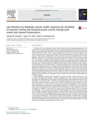
  • 4. 264 A.M. Palumbo et al. / Icarus 300 (2018) 261–286 Table 1 Important abbreviations utilized in this paper. In this paper, we focus on seasonal and diurnal temperature variations, as illustrated in Fig. 1. For convenience, we will utilize multiple abbreviations in our analysis, all of which are described in the table. Mean annual temperature (MAT) The average temperature throughout the entire year at a specified latitude and longitude. Global MAT is the average temperature throughout the entire year for the whole globe. For example, a nominal “cold and icy” climate has global MAT of ∼225 K (e.g. Wordsworth et al., 2013). Peak annual temperature (PAT) The warmest temperature experienced throughout the year at a specified longitude and latitude. In other words, PAT corresponds to the warmest “data point” from the GCM simulation. Peak daytime temperature (PDT) The warmest temperature reached within a given day at a specified latitude and longitude. We use this term when discussing diurnal temperature variation. For example, the PDT for a day in the middle of the winter will be much colder than the PDT for a day in the middle of the summer. Mean seasonal temperature (MST) The average temperature throughout one of the four seasons at a specified latitude and longitude. To illustrate this, consider a fictional example of a region with MAT below the melting point of water. In this case, liquid water will not be stable on the surface throughout the year. However, summertime conditions will be warmer than annual averages, and it is possible that summertime MST are above 273 K, permitting the stability of liquid water at the surface for at least half of the summer season. Peak seasonal temperature (PST) The maximum temperature reached throughout a specific season. We collect GCM data every six model hours, so this value represents the absolute warmest six hours of the specific season. Positive degree day (PDD) For the purpose of this analysis, we consider a day to be a PDD if it has at least 6 consecutive hours with an average temperature above 273 K (in other words, one data point). Fig. 1. A cartoon illustrating the relationship among mean annual temperatures (MAT), peak annual temperatures (PAT), mean seasonal temperatures (MST), and peak seasonal temperatures (PST). PAT can be much higher than MAT, reflecting the absolute warmest time recorded during the year. Additionally, MST can be much higher than MAT (as shown here for the summer season), or much lower (as shown here for the winter season). This example is a possible sketch for a MAT of 225 K, typical for a Late Noachian “cold and icy” climate scenario. Note that the warmest days of the summer season (PAT) experience temperatures > 273 K. climate. Their simulation with spin-axis and pressure conditions similar to the Noachian (their simulation p128x_std: conditions of 25° obliquity and 1200 mbar CO2 atmosphere) produces warm conditions with temperatures consistently above the melting point of water and continuous stability of liquid water at the surface. We suggest that these results are related to the nature of their model, which causes over-prediction of temperatures for the reasons out- lined above (e.g. over-effective greenhouse warming, assumption of current solar luminosity, and not accounting for radiative effects of CO2 or H2O clouds). In this analysis, we consider the ambient “cold and icy” conditions which are predicted by our updated model, in which temperatures only exceed 273 K in the warmest hours of the summer season in a few places on the planet. The duration and distribution of these temperature conditions with respect to obliquity, pressure, and eccentricity are of critical importance to our analysis. In order to better understand seasonal temperature variations on early Mars, we must first consider conditions on Earth. The Earth’s current global MAT is ∼287 K, but local MAT can reach 330 K in the hottest deserts and plummet as low as 184 K in Antarctica, at the South Pole. Thus, in addition to MAT, it is use- ful to explore peak temperatures, the range of temperatures, and how they vary with season (Fig. 1). In addition to MAT, we suggest that it is also important to explore peak annual temperature (PAT; the highest daily temperature reached in a year), mean seasonal temperatures (MST; for example, MAT could be well below 273 K, but MST > 273 K for the summer season), peak daily temperature (PDT; the highest temperature reached in each day), and peak sea- sonal temperature (PST; the highest temperature reached in each season). All abbreviations utilized in this analysis, such as those previously mentioned, are included in Table 1 with corresponding definitions. In the Antarctic McMurdo Dry Valleys (MDV), for example, MAT (∼253 K) is well below the melting point of water (273 K), yet PAT can exceed 273 K (e.g. Head and Marchant, 2014). Indeed, peak daytime temperatures (PDT) can exceed 273 K for many weeks of southern summer, top-down melting of snow and ice can occur, and resultant meltwater-related fluvial and lacustrine activity can produce observable landforms and deposits, all in the absence of pluvial activity (Marchant and Head, 2007; Head and Marchant, 2014). Over much of the MDV in southern summer, PDT can exceed 273 K, but there is commonly no surface snow and ice to melt, and the duration of the period > 273 K is insufficient for the warming thermal wave to penetrate the dry active layer and melt the ice- cemented portion of the cryosphere (Head and Marchant, 2014). Thus, formation of the fluvial and lacustrine features in the Mars- like hyperarid-hypothermal environment of the MDV requires not only PDT exceeding 273 K, but also the presence of localized sur- face deposits of snow and ice to melt (Head and Marchant, 2014). We use the MDV as a guideline for conditions that need to per- sist in a “cold and icy” early Mars climate in order for the ob- served martian fluvial/lacustrine features to form (Palumbo and Head, 2017b). A factor in transient melting of the tops of cold-based glaciers in the MDV is changes in the ice albedo related to deposits on the snow and ice (Chinn, 1986; Fountain et al., 1999; Aitkins and Dick- inson, 2007; Marchant and Head, 2007; Head and Marchant, 2014). The presence of rocks, dust and dirt on the ice deposit decreases the albedo of the “dirty” ice deposit, in turn increasing the amount of solar radiation absorbed by the “dirty” ice, potentially producing meltwater at surface air temperatures lower than 273 K, depend- ing on the thickness of the deposit and other factors (Wilson and Head, 2009) which are not well constrained for the Noachian en- vironment. The dust particles themselves will warm from solar ra- diation and possibly melt surrounding ice. Dust (including volcanic tephra) may have influenced ice in the Noachian (Cassanelli et al., 2015; Wilson and Head, 2009). This topic is not included in this analysis but is currently being assessed. Additionally, Gooseff et al. (2017) have analyzed the influence of an anomalously warm year, 2002, on the physical and ecologi- cal states of the MDV. They find that the uncharacteristically warm summertime temperatures produced a significant response in the Antarctic system, with increases in lake levels and stream fluxes.
  • 5. A.M. Palumbo et al. / Icarus 300 (2018) 261–286 265 This anomalously warm year has proven to be a turning point in the MDV climate: the climate was cooling before 2002, and has been warming since 2002. While some factors in the MDV system experienced delayed responses to the 2002 austral summer, such as microbial mats and select species of Antarctic nematodes, the rivers and lakes appeared to have an immediate response, with lake levels and stream fluxes increasing immediately during the 2002 austral summer. Thus, we must also consider that anoma- lously warm years, such as the conditions experienced in 2002 in the MDV, may be sufficient to induce significant transient overland flow and contribute to the formation of fluvial features in a com- parable Noachian climate scenario. To address our question regarding potential seasonal melting in the “Late Noachian Icy Highlands” (LNIH) climate model, we use the 3-Dimensional Laboratoire de Météorologie Dynamique (LMD) GCM for early Mars to explore the hypothesis that peak annual, daytime or seasonal temperatures (PAT, PDT, or PST) in a “cold and icy” Late Noachian climate (Forget et al., 2013; Wordsworth et al., 2013) with MAT ∼225 K could produce transient snowmelt and subsequent runoff in sufficient quantities and at the appropriate locations to explain the nature and distribution of valley networks and related lacustrine features. We focus on several specific ques- tions: (1) In past Mars climate history when the MAT is predicted to be <<273 K, do temperatures ever exceed 273 K, for example, in the summer season? (2) If seasonal temperatures exceed 273 K in the MAT ∼225 K scenario, but are insufficient to induce prolonged pluvial (rainfall) activity, are peak annual and peak seasonal tem- peratures (PAT/PST) sufficiently high and of a sufficient duration to cause melting of surface snow and ice? (3) How much meltwater is produced through this mechanism annually and how does this compare to the volume of water and runoff rates required to form the valley networks? 2. Methods and approaches 2.1. General model features To complete our study, we used the 3D LMD GCM for early Mars (e.g. Wordsworth et al., 2013; Forget et al., 2013). This finite-difference model uses atmospheric radiative transfer, mete- orological equations, and physical parameterizations in conjunc- tion with one another. The model incorporates cloud microphysics with a fixed cloud condensation nuclei number density scheme for H2O and CO2 cloud particles (Wordsworth et al., 2013; Forget et al., 2013), convective processes (Wordsworth et al., 2013; Forget et al., 2013), and precipitation (Wordsworth et al., 2015; following Boucher et al., 1995). Because of the uncertainties in the nature and distribution of Noachian dust, we do not include the effects of a dusty snow and ice layer here, although we recognize that the addition of dust in our simulations may aid in seasonal melting in a “cold and icy” climate (Clow, 1987; Cassanelli et al., 2015). Additionally, Kreslavsky and Head (2000, 2003, 2006) have highlighted the im- portance of surface slopes in seasonal melting. We acknowledge that the difference of incident solar radiation between equator- facing and pole-facing slopes may be substantial. The GCM uses MOLA topography data to account for regional slope variation, however, the resolution of the model utilized here precludes us from exploring the influence of this in more detail, and is a topic of future work. For the purpose of this study, we track surface temperature and H2O ice with a spatial resolution of 64 × 48 × 18 (longi- tude × latitude × altitude), which is a sufficient spatial resolution to capture the necessary regional temperature variations, and collect hourly data, which is a sufficient temporal resolution to capture diurnal and seasonal temperature variation. 2.2. Approaches and specific applications We employ the LMD GCM to test for transient melting un- der the conditions of PAT. In this analysis, we focus on a range of pressures (600–1000 mbar) for a pure CO2 atmosphere (e.g. Forget et al., 2013), and we explore the effects of a range of spin-axis obliquities (25°−55°; ±1σ of the mean obliquity over the past 5 billion years as estimated through a statistical analy- sis by Laskar et al., 2004) and eccentricities (0–0.17; lower and upper limit represent statistically probable values for the past 5 billion years with eccentricity 0.17 having ∼20% probability; Laskar et al., 2004), assuming a solar luminosity 75% of the cur- rent value (Gough, 1981; Sagan and Mullen, 1972). It is important to note that Laskar et al. (2004) considered a statistical model, esti- mating probable mean values and ranges (one standard deviation) for spin-axis/orbital parameters. However, it is probable that these parameters, such as obliquity and eccentricity, varied to values out- side the statistically probable range. We recognize that there was likely to be more variation than that suggested by the statistical analysis performed by Laskar et al. (2004), but for the purpose of this study we focus on the range estimated by Laskar et al. (2004), as described above. We specifically analyze 600 mbar, 800 mbar, and 1000 mbar atmospheres, each at obliquities of 25°, 35°, 45°, and 55° and ec- centricities of 0 (circular) and 0.17. In exploring this parameter space, we utilize surface temperature variation as a proxy to assess whether transient melting of snow and ice could be responsible for valley network formation in areas where Late Noachian snow ac- cumulation is well correlated with the valley network distribution (Wordsworth et al., 2015). We also consider the addition of a small amount of greenhouse gas surrogate in the atmosphere, an addi- tion that serves to strengthen the annual warming effect, to assess how much annual warming above 273 K could occur under condi- tions where MAT is greater than 225 K but still below 273 K. In this part of our analysis, our goal is to assess a climate scenario that is warmer than the baseline “cold and icy” climate (∼225 K MAT), but still not continuously “warm and wet” (MAT > 273 K); this climate scenario is still broadly characterized by ice and snow distributed in the highlands and MAT far below the melting point of water. Be- cause of uncertainty in sources and sinks for specific greenhouse gases, we account for additional greenhouse warming by adding gray gas, which absorbs evenly across the spectrum at a defined absorption coefficient. We choose a small absorption coefficient to raise MAT by only a few degrees, maintaining an overall “cold and icy” climate scenario. Lastly, we also explore additional scenarios for completeness and to consider extreme conditions, including a low obliquity (15°) simulation and a high eccentricity simulation (0.2; estimated maximum value reached in the past 5 billion years based on the statistical analysis of Laskar et al., 2004). Seasonal temperature variation has been proven to be impor- tant in the recent Mars climate scenario (Richardson and Mis- chna, 2005). In our analysis we are using a more advanced model, including a water cycle, radiative effects of CO2 and H2O clouds, and decreased solar luminosity, to adequately test whether this importance extends throughout martian history and back to the Noachian. These results also lay the basis for determining whether repetitive yearly peak temperature melting events, in similar loca- tions over long periods of time, could be responsible for more sig- nificant fluvial/lacustrine activity if yearly amounts of melting are insufficient to explain the entire valley network landscape, a situa- tion that is observed in the MDV (Head and Marchant, 2014). In this analysis, we first search for regions with substan- tial snow accumulation that also have PAT > 273 K, permitting snowmelt and runoff at these locations. By comparing regions of PAT > 273 K and the predicted LNIH ice distribution, we place further constraints on the spin-axis/orbital parameter space
  • 6. 266 A.M. Palumbo et al. / Icarus 300 (2018) 261–286 Fig. 2. Global maps of the mean (column A) and peak (maximum) (column B) annual temperature for a pure CO2 atmosphere and a circular orbit. Shown are these mean and maximum values in conditions of different obliquity (rows 1 and 2 at 25° obliquity; rows 3 and 4 at 45° obliquity) and different atmospheric pressure (rows 1 and 3 at 600 mbar; rows 2 and 4 at 1000 mbar). Column B also shows regions with peak annual temperature > 273 K outlined in white. The purpose of this is to highlight regions with peak temperatures above the melting point of water. All data shown here are taken from model year 10. Note (1) the increase in surface area > 273 K as atmospheric pressure increases and (2) the north poleward shift of warm temperatures as obliquity increases. Column B illustrates the fact that the highest percentage of the equatorial region with PAT > 273 K occurs for low obliquity (25°) and high atmospheric pressure (1000 mbar). Although higher obliquity conditions (45°) for the same atmospheric pressure (1000 mbar) produces a higher percentage of the planet with peak annual temperatures above 273 K, we consider the lower obliquity case as optimal conditions for valley network formation because more of the equatorial region experiences peak annual temperatures > 273 K. necessary to maximize any transient melting in the equatorial re- gions where valley networks are abundant. Next, we determine the annual duration of melt conditions at specific valley network sys- tems to constrain better the applicability of this mechanism to val- ley network formation. The valley network systems chosen for this study are distributed near the edges of the predicted ice sheet and are locations that would require melting of ice and surface runoff to form in the “cold and icy” climate scenario. Last, we estimate the volume of meltwater produced annually through this mecha- nism (for optimal spin-axis/orbital and atmospheric pressure con- ditions). We then compare this with the total water volume be- lieved to be required to form the valley networks and lakes to pre- dict the total duration necessary for such a meltwater process to form these features. We also explore the magnitude of runoff rates produced by this mechanism to hypothesize whether they would be sufficient to form the valley networks and further narrow down which spin-axis/orbital and atmospheric pressure conditions are most suitable to valley network formation. In summary, we use the 3D LMD GCM to better understand the role of seasonal temperature variations and the potential for the production of meltwater during peak summertime conditions. We explore climate variation and possible formation of fluvial and lacustrine features in a manner similar to how they form in the MDV; we do this by focusing on peak instead of mean annual temperatures and assessing whether warm summertime conditions could produce a significant quantity of meltwater. Additionally, we offer an expansion on the previously explored parameter space of early Mars climate (e.g. Richardson and Mischna, 2005; Forget et al., 2013; Wordsworth et al., 2013; Wordsworth et al., 2015) by studying the implications for both variations in eccentricity and moderate greenhouse warming in a “cold and icy” climate. 3. Analysis We now explore the parameter space for specific spin- axis/orbital conditions, namely both 25° and 45° obliquities, each with 600 and 1000 mbar CO2 atmospheres, at eccentricities 0 and
  • 7. A.M. Palumbo et al. / Icarus 300 (2018) 261–286 267 Fig. 3. Global maps of the mean (column A) and peak (maximum) (column B) annual temperature for a pure CO2 atmosphere and an orbit with eccentricity of 0.17, which is a statistical upper limit (20% probably of occurring in the past 5 billion years) for martian eccentricity during the Noachian (Laskar et al., 2004). Here we consider a longitude of perihelion of Ls = 90. Compare to Fig. 2 which shows the same maps for a circular orbit. The increased eccentricity results in longer and warmer summer seasons (specifically in the northern hemisphere during higher obliquity), producing larger regions of PAT > 273 K than for a circular orbit (Fig. 2) under similar spin-axis/orbital and pressure conditions. Fig. 4. The distribution of valley networks and the predicted distribution of snow and ice in the LNIH model. Valley network distribution map (red lines; Hynek et al., 2010) superposed on the predicted “Late Noachian Icy Highlands” ice distribution at 1 km ELA (equilibrium line altitude) (Head and Marchant, 2014). The locations of the three valley networks sites analyzed in this study are shown. Topography is MOLA data (brown is high, purple is low). (For interpretation of the references to color in this figure legend, the reader is referred to the web version of this article.)
  • 8. 268 A.M. Palumbo et al. / Icarus 300 (2018) 261–286 0.17. These cases represent (1) both a low obliquity (25°) and the most probable average Noachian obliquity (45°, most likely obliq- uity is 41.8°; Laskar et al., 2004), (2) relatively low and high at- mospheric pressure values (600 and 1000 mbar), and (3) the full range of probable eccentricity values (0 and 0.17). The model is run, with fixed conditions, for 10 years; all model data are taken from model year ten or higher to ensure equilibration of the model parameters utilized here. We utilize hourly data to ensure that we are capturing the warmest daily temperatures. 3.1. Pure CO2 atmosphere 3.1.1. Mean annual temperatures (MAT) and peak annual temperatures (PAT) The global distribution of MAT (globally averaging ∼225 K) predicted by our GCM analyses is shown for 25° obliquity and 600 mbar (Fig. 2a-1). For the remainder of this discussion, we will refer to the column as its corresponding letter and the row as its corresponding number; for example, Fig. 2a-1 implies Fig. 2, col- umn a, row 1), 25° obliquity and 1000 mbar (Fig. 2a-2), 45° obliq- uity and 600 mbar (Fig. 2a-3), and 45° obliquity and 1000 mbar (Fig. 2a-4) for a circular orbit and, similarly, repeated for the same spin-axis and atmospheric pressure conditions for the higher ec- centricity value (eccentricity of 0.17; Fig. 3a-1–4 has perihelion at Ls = 90 or northern hemispheric summer, and Fig. 5a-1–4 has per- ihelion at Ls = 270 or southern hemispheric summer). Within this parameter space, the equilibrated ice distribution is that derived for a “Late Noachian Icy Highlands” scenario (Wordsworth et al., 2013, 2015) (Fig. 4). With global MAT (∼225 K) far below (48 K) the 273 K melting point, we ask the question: Could PAT exceed 273 K in the warmest parts of the year, the melting point of pure water ice? To evaluate this question and determine whether or not tem- peratures exceed 273 K at any point on Mars during the year, we produced PAT maps showing the peak annual temperature at every pixel across the globe for each of the four aforementioned studied cases (Figs. 2b-1–4, 3b-1–4, 5b-1–4). Our analysis shows that peak annual temperatures exceed 273 K somewhere on Mars during the year in all cases treated (600–1000 mbar, 25–55° obliquity, 0–0.17 eccentricity). First, we consider the case of a circular orbit (eccentricity of 0, Fig. 2). How does PAT change with increasing CO2 atmospheric pressure? As the amount of CO2 in the atmosphere increases, the greenhouse effect becomes stronger and peak temperatures become more significant, increasing across the planet (compare Fig. 2b-1 and 2b-2). Also, as the total atmospheric pressure in- creases, the amplitude of the diurnal cycle decreases somewhat because the atmospheric heat capacity is larger. This mechanism acts to counteract the increased CO2 greenhouse effect on the diurnal timescale, making it more difficult for temperatures un- der a thicker atmosphere to reach daytime conditions > 273 K for MAT < 273 K. However, the strengthened greenhouse effect is the more powerful mechanism at play under these spin-axis/orbital conditions and thus, the increased CO2 atmospheric pressure cor- responds to a global increase in both MAT and PAT. At 25° obliq- uity and 600/1000 mbar pressure (Fig. 2b-1, 2b-2), PAT > 273 K oc- currences are concentrated mostly in the northern lowlands and the floors of the Hellas and Argyre impact basins due to the alti- tude dependence on temperature. Temperatures across the planet increase with increasing atmospheric pressure (1000 mbar) and, thus, the percentage of the planet with PAT > 273 K also increases (compare Fig. 2b-1 and 2b-2, regions outlined in white). For exam- ple, for 25° obliquity and 600 mbar conditions (Fig. 2b-1), ∼22.8% of the planet has PAT > 273 K, but with increased atmospheric pres- sure (1000 mbar) (Fig. 2b-2), the percentage of the planet with PAT > 273 K increases to ∼28.4%. This trend is illustrated in Fig. 2b, where all regions with PAT > 273 K are outlined in white. Compar- ison of the PAT distribution plots with a map of the predicted dis- tribution of snow and ice in the LNIH model (Fig. 4) and the dis- tribution of valley networks (Fig. 4) shows that a few areas with both snow and valley networks correspond to the regions of PAT that exceed 273 K (compare Figs. 2b-1–4 and 4). Noteworthy is the fact that maximum temperatures (see PAT maps, Fig. 2b) in the northern lowlands are higher at higher obliq- uity due to the latitudinal effects of solar insolation with increas- ing obliquity. This is illustrated in Fig. 2b-1 (25° obliquity and 600 mbar CO2 atmosphere) and Fig. 2b-3 (45° obliquity and 600 mbar CO2 atmosphere). At lower (25°) obliquity, the highest maximum temperatures are located closer to the equator, while at higher (45°) obliquity, the highest maximum temperatures have shifted toward the poles. Although the results of our highest obliquity simulations (55°) are not shown in Fig. 2, the results are substan- tively the same as those of the 45° obliquity simulations, with maximum temperatures shifted slightly more towards the poles. Next, we repeat our study for the case of a more eccentric orbit (Fig. 3, perihelion at Ls = 90; Fig. 5, perihelion at Ls = 270) (eccen- tricity of 0.17, upper limit of our analyzed eccentricity range be- cause higher eccentricities have less than 20% probability of hav- ing occurred in the past 5 billion years; Laskar et al., 2004). This eccentricity range has not been studied in full detail previously, and thus our analysis provides important information about the influence of eccentricity on climate. For example, in a more ec- centric orbit, the strength of the seasonal cycles increases and, de- pending on the perihelion conditions, one hemisphere will experi- ence a warmer summer than in the circular orbit scenario. In other words, for simulations where perihelion occurs during southern hemispheric summer (longitude of perihelion of Ls = 270), sum- mertime temperatures in the southern hemisphere are increased because the planet is closer to the Sun during the summer sea- son and farther from the Sun during the winter season, as com- pared to a less eccentric, or circular, orbit. Thus, in the higher ec- centricity scenario, peak summer temperatures increase and peak winter temperatures decrease for the hemisphere that experiences the summer season during perihelion. Understanding the conse- quences that variations in eccentricity have on MAT and PAT dis- tributions is important for this study because increasing eccentric- ity increases peak summertime temperatures for the hemisphere that is in the summer season during perihelion, potentially per- mitting the production of more seasonal meltwater than in the circular orbit case. Additionally, the precession timescale is ∼50 ky, significantly shorter than the estimated timescale for forma- tion of simple valley networks (∼108 years total; Hoke et al., 2011). To remedy this, we analyze two datasets of opposite perihelion to better understand the influence of eccentricity variation and analyze the dataset by assuming that both perihelion scenarios persist for approximately half of the duration of valley network formation. The two perihelion scenarios that we consider in this analysis are (1) perihelion at Ls = 90, or northern hemispheric summer, and (2) perihelion at Ls = 270, or southern hemispheric summer. The overall temperature distribution patterns observed in the circular orbit case are also observed here for the more ec- centric case (Fig. 3; northern hemispheric summer at perihe- lion). As obliquity increases from 25° to 45° (compare Fig. 3b- 1 and 3b-3), PAT increase in the polar regions and decrease in the equatorial region (for example, compare Fig. 3a-2 and Fig. 3a-4). However, in the higher eccentricity scenario, the ef- fects of thermal blanketing by higher atmospheric pressure ap- pear to significantly decrease the amplitude of the diurnal cycle. Thus, in contrast to the circular orbit scenario, as atmospheric pressure increases from 600 to 1000 mbar (compare Fig. 3a- 1 and 3a-2), although MAT across the globe increase by ∼10 K,
  • 9. A.M. Palumbo et al. / Icarus 300 (2018) 261–286 269 Fig. 5. Same as Fig. 3, except showing the reversed perihelion simulations (longitude of perihelion Ls = 270). the area of the region with PAT > 273 K does not increase sig- nificantly (compare regions outlined in white in Fig. 3b-1 and 3b-2 or Fig. 3b-3 and 3b-4). For example, approximately the same percentage of the globe is characterized by PAT > 273 K at 45° obliquity and 600 mbar (Fig. 3b-3) and 45° obliquity and 1000 mbar (Fig. 3b-4). In a manner similar to circular orbit con- ditions, under these spin-axis/orbital conditions, PAT > 273 K oc- curs both in the northern hemisphere and in equatorial regions where valley networks are abundant (see Fig. 3b and compare to Fig. 4). PAT in the southern hemisphere are lower than PAT in the northern hemisphere because of the altitude dependence of temperature and because the longitude of perihelion (Ls = 90) is such that the northern hemisphere experiences summer at perihelion and the southern hemisphere experiences summer at aphelion. In simulations where the perihelion occurs at Ls = 270 (Fig. 5; southern hemispheric summer at perihelion), we observe simi- lar patterns to those observed in the previous simulations. As a consequence of the perihelion conditions, PAT in the southern hemisphere are warmer than in both the circular orbit and the reversed perihelion simulations; in significant portions of the southern hemisphere PAT exceed 273 K (Fig. 5b). This perihelion scenario (longitude of perihelion of Ls = 270) is critical to sum- mertime melting because southern hemispheric summer occurs at perihelion; since a significant portion of the Noachian ice sheet was likely distributed in the southern hemisphere, this perihelion scenario can produce significantly more meltwater than the peri- helion scenario in which northern hemispheric summer occurs at perihelion. Our initial study of temperature distributions suggests that increasing the eccentricity to 0.17 introduces significantly more seasonal warming (see Figs. 3 and 5) than for conditions of a circular orbit; the percentage of the planet with PAT > 273 K is greater than in the case of a circular orbit. For example, for the conditions of a 600 mbar CO2 atmosphere and 25° obliq- uity, 22.8% of the planet experiences PAT > 273 K when consid- ering a circular orbit, and up to 33.4% of the planet experi- ences PAT > 273 K when considering an orbit with eccentricity of 0.17 (for conditions of perihelion occurring during southern hemispheric summer). Additionally, variations in perihelion con- trol where the meltwater will be concentrated, depending upon which hemisphere is experiencing the summer season when Mars approaches perihelion. In summary, throughout the parameter space explored (atmo- spheric pressure, obliquity, eccentricity), PAT greater than or equal to 273 K (regions outlined in white in Figs. 2, 3, and 5) occur in the northern lowlands, topographic lows such as the floors of basins, and parts of the equatorial region, but equatorial temper- atures > 273 K only partially spatially correlate with regions where valley networks are observed (Fig. 2b1–4, 3b1–4, 5b1–4; compare to Fig. 4). For the case of a circular orbit, as obliquity increases, the highest MAT and PAT begin to shift towards the pole and as at- mospheric pressure increases, the greenhouse effect increases, thus increasing MAT and the percentage of the globe with PAT > 273 K.
  • 10. 270 A.M. Palumbo et al. / Icarus 300 (2018) 261–286 Fig. 6. Temperature time series (one martian year duration, beginning at Ls = 0) for all conditions studied in Fig. 2 (circular orbit) at three different valley network systems distributed at different latitudes and longitudes (see Fig. 4 for locations). Column A is 25° obliquity and 600 mbar CO2. Column B is 25° obliquity and 1000 mbar CO2. Column C is 45° obliquity and 600 mbar CO2. Column D is 45° obliquity and 1000 mbar CO2. Valley network locations are 1 (top) Evros Valles (12°S, 12°E), 2 (middle) the valley networks near the Kasei Outflow Channels (23°N, 55°W), and 3 (bottom) Parana Valles (24.1°S, 10.8°W). Horizontal lines at 273 K provide a reference to show how close PAT approach the melting point of water. Green lines highlight examples when temperatures approach (temperatures exceed 265 K at some point during the year) or are above 273 K for at least one data point during the year. Red lines indicate when temperatures approach, but do not exceed 273 K (temperatures are consistently below 265 K). Note that all horizontal lines are green. (For interpretation of the references to color in this figure legend, the reader is referred to the web version of this article.) In other words, lower obliquity conditions permit warmer temper- atures in the equatorial region (where valley networks are most abundant), and higher pressure increases temperature globally, in- creasing the percentage of the planet with PAT above the melting point of water. Based on these results and thermal considerations for the production of meltwater, we predict that the optimal spin- axis/orbital conditions to produce equatorial melting are relatively low obliquity and elevated atmospheric pressure. For the case of a more eccentric orbit (eccentricity 0.17), the same obliquity ef- fects are observed, but as atmospheric pressure increases, increas- ing the greenhouse effect, the increased thermal blanketing signif- icantly decreases the diurnal cycle and, although MAT increases on a global scale, the percentage of the globe with PAT > 273 K does not significantly increase. Higher eccentricity increases the possibility of seasonal summertime melting in regions with abun- dant valley networks for conditions characterized by perihelion at southern hemispheric summer, because significant meltwater can be produced in the southern hemisphere. Thus, higher eccentricity conditions are more optimal for the production of meltwater in re- gions with abundant valley networks than circular orbit conditions. 3.1.2. Valley network analysis: temperature time series Our exploration of parameter space has shown that PAT in ex- cess of 273 K, and thus areas conducive to melting of surface snow and ice, can occur in equatorial regions where valley networks are observed (Fig. 4). Uncertain, however, is whether these tempera- tures will persist long enough to create significant melting and subsequent surface runoff. In order to produce the maximum tem- perature plots shown in Fig. 2b (and Figs. 3b and 5b for eccen- tricity of 0.17), we sampled the maximum temperature reached throughout the year at each lat/lon model grid point. We ask the question: Do temperatures > 273 K occur at more than one data
  • 11. A.M. Palumbo et al. / Icarus 300 (2018) 261–286 271 Fig. 7. Temperature time series (one martian year duration) for all conditions studied in Fig. 3 (orbital eccentricity of 0.17, longitude of perihelion of Ls = 90) at three different valley network systems distributed at different latitudes and longitudes (see Fig. 4 for locations). Column A is 25° obliquity and 600 mbar CO2. Column B is 25° obliquity and 1000 mbar CO2. Column C is 45° obliquity and 600 mbar CO2. Column D is 45° obliquity and 1000 mbar CO2. Valley network locations are 1 (top) Evros Valles (12°S, 12°E), 2 (middle) the valley networks near the Kasei Outflow Channels (23°N, 55°W), and 3 (bottom) Parana Valles (24.1°S, 10.8°W). Horizontal lines at 273 K provide a reference to show how close PAT approach the melting point of water. Green lines highlight examples when temperatures approach (temperatures exceed 265 K at some point during the year) or are above 273 K for at least one data point during the year. Red lines indicate when temperatures approach, but do not exceed 273 K (temperatures are consistently below 265 K). Note that all horizontal lines are green. (For interpretation of the references to color in this figure legend, the reader is referred to the web version of this article.) point (on the time domain; e.g. one data point is collected ev- ery model hour) during the martian year, suggesting that temper- atures > 273 K persist for more than just the warmest hour of the warmest day in the summer season? In order to assess the dura- tion of temperatures > 273 K at each lat/lon model grid point, we collected model data 24 times per martian day (hourly), 16,056 times per martian year. While the PAT maps represent only one data point, it is possible that, at locations where PAT > 273 K (Figs. 2, 3, 5), temperatures > 273 K may occur at more than one data point during the year, suggesting a longer duration of conditions suitable to melting of surface ice. In fact, such conditions would be required to produce sufficient melting and runoff to form the observed fluvial and lacustrine features. To determine whether the PAT values at each lat/lon grid point correspond to a single data point, a few data points, or a summer average, we produced tem- perature time series for one model martian year. We do this for all the previously described obliquity, pressure, and eccentricity con- ditions (Fig. 6, circular; Fig. 7, eccentricity 0.17 with perihelion at Ls = 90; Fig. 8, eccentricity of 0.17 with perihelion at Ls = 270). For this part of the analysis, we focus on three specific val- ley network systems (locations shown in Fig. 4): (1) Evros Valles (12°S, 12°E), (2) valley networks near the Kasei outflow chan- nels (referred to as the Kasei site; 23°N, 55°W), and (3) Parana Valles (24.1°S, 10.8°W). We chose examples at these different lon- gitudes and latitudes in order to obtain a global sampling of re- gions where valley networks are abundant and to assess the per- centage of the year that these different areas experience temper- atures in excess of 273 K. In the MDV, for example, temperatures
  • 12. 272 A.M. Palumbo et al. / Icarus 300 (2018) 261–286 Fig. 8. Temperature time series (one martian year duration) for all conditions studied in Fig. 5 (orbital eccentricity of 0.17, longitude of perihelion of Ls = 270). Note that, under some conditions at some locations, horizontal lines are red; temperatures are consistently below 265 K. (For interpretation of the references to color in this figure legend, the reader is referred to the web version of this article.) above 273 K are achieved during only a few percent of the year, and yet fluvial features similar to those on Mars are observed to form and persist from year to year (Head and Marchant, 2014). We have analyzed Long Term Ecological Research (LTER) climate mon- itoring data for Lake Hoare, in Taylor Valley of the MDV (https:// lternet.edu/sites/mcm), and find that (1) under average annual conditions—where both MAT and PAT are comparable to adjacent years—approximately 5–7% of the year is characterized by surface temperatures > 273 K; and (2) under warmer than average annual conditions—where both MAT and PAT are slightly higher than ad- jacent years—approximately 11% of the year is characterized by surface temperatures greater than 273 K. Although these ambi- ent Antarctic conditions are of course not directly comparable to Noachian “cold and icy” conditions because the MDV climate sce- nario is driven by seasonal temperature variation and lacks sig- nificant diurnal variation, we use the fact that transient seasonal warming for a minimum of ∼5–7% of the year is a duration that permits local seasonal melting of accumulated snow and ice and leads to transient fluvial and lacustrine activity in the MDV as a broad interpretive guideline for this study. First, we focus on the case of a circular orbit (Fig. 2). Fig. 6 shows temperature time series at the three valley network sample locations, and encompassing one martian year, for the con- ditions shown in Fig. 2. In all figures representing the results of our valley network analysis (Fig. 6 corresponds to circular orbit condi- tions; Figs. 7 and 8 correspond to eccentricity of 0.17 with perihe- lion at Ls = 90 and Ls = 270, respectively), the horizontal lines show the location of the 273 K ice melting temperature; the horizontal lines are green when temperatures approach the melting point of water (temperatures exceed 265 K at some point during the year) and red when temperatures do not approach the melting point of water (temperatures never exceed 265 K). The green lines at 273K in all panels in Fig. 6 show that temperatures approach the melt- ing point at all locations under all spin-axis conditions (tempera- tures exceed 265 K at some point during the year). However, these time series plots (Fig. 6) show that, at these three valley network
  • 13. A.M. Palumbo et al. / Icarus 300 (2018) 261–286 273 locations, melting conditions (273 K) are either never reached or, if they are reached, only last for a few data points per year. Because we utilize hourly data in this analysis, it is possible that the data points above 273 K represent peak day time conditions from the warmest days in the summer season. Thus, with only a few data points above 273 K, we conclude that these conditions permit only one or a few days per year where melting conditions are reached during peak day time conditions. When we compare this to the conditions required to form similar fluvial and lacustrine features in the MDV, such a short annual period of melting would likely be insufficient to form the observed martian fluvial and lacustrine surface features. Under some conditions, however, such as 25° obliquity and a 1000 mbar CO2 atmosphere (Fig. 6), the valley networks near the Kasei site hover just below 273 K for a more significant portion of the year (for example, 22 days have maximum temperatures greater than or equal to 265 K, approximately 3.3% of the year). Seasonal variation in temperature in the MDV, where fluvial fea- tures are present, imply that, while melting conditions are not persistent, being close to the melting point for approximately one season could allow for fluvial features to form or persist under spe- cific conditions (Head and Marchant, 2014). However, this scenario requires one season, or ∼25% of the year, to have temperatures close to the melting point (in other words, summer PST ∼273 K), which is much more than the model simulations suggest for these early martian spin-axis/orbital and pressure conditions. Therefore, although temperatures can be close to 273 K for multiple days in the summer season, we conclude that the duration is still not suf- ficient to sustain fluvial and lacustrine features under conditions of a pure CO2 atmosphere and a circular orbit. Next, we focus on the case of a more eccentric orbit, with ec- centricity of 0.17 (Fig. 7, perihelion occurs at Ls = 90; Fig. 8, peri- helion occurs at Ls = 270). As previously mentioned, the increased eccentricity leads to more extreme seasonal cycles, and thus to increased PAT due to warmer summertime conditions. This is ex- pressed in the form of (1) a higher percentage of the planet char- acterized by PAT > 273 K, and (2) a difference in number of days in which temperatures rise above 273 K at the valley network lo- cations studied. Locations that never reach 273 K in the circular orbit are now characterized by temperatures greater than 273 K, sometimes for multiple days depending on which hemisphere ex- periences summertime during perihelion (Figs. 7 and 8). For ex- ample, the Kasei site experiences less time above freezing than Parana Valles for conditions of southern hemispheric summer at perihelion (Fig. 8). A significantly higher percentage of the year is characterized by temperatures > 273 K at the valley network lo- cations for the case of a more eccentric orbit, with values more similar to what is observed in the MDV (maximum 25 days with PAT > 273 K at the Kasei site (∼4% of the year), maximum 30 days with PAT > 273 K at Parana Valles (∼4.5% of the year), and maxi- mum 22 days with PAT > 273 K at Evros Valles (∼3% of the year); the maximum values are taken as the maximum value from either perihelion scenario). Thus, the results from the simulations with eccentricity of 0.17 are more promising for the production of sig- nificant summertime melting than that of a circular orbit and we explore these conditions further in a later section. There are some conditions which result in a greater portion of the year with temperatures temporarily stabilized just below 273 K, in a manner similar to the case of a circular orbit. For ex- ample, at 25° obliquity and a 600 mbar CO2 atmosphere with ec- centricity of 0.17 and perihelion at Ls = 90, Parana Valles experi- ences PDT > 265 K for ∼71 days (approximately 11% of the year). Under these same conditions, Evros Valles experiences PDT > 265 K for ∼69 days (approximately 10% of the year) and the valley networks near the Kasei site experience PDT > 265 K for ∼88 days (approximately 13% of the year). Thus, a significantly higher per- centage of the summer season is characterized by temperatures that approach 273 K for increased eccentricity conditions. Although these conditions persist for a period much less than one season and there is likely to be significantly more diurnal temperature variation than observed during the summer season in the MDV, we consider that increased eccentricity conditions warrant fur- ther consideration when considering seasonal summertime melt- ing (Head and Marchant, 2014). In conclusion, when considering an eccentric orbit (0.17), the magnitude of the seasonal cycle is enhanced and significant seasonal melting can ensue, producing a number of days with PAT > 273 K at different valley networks that is comparable to what is observed in the MDV. However, when considering a circular or- bit, although a “cold and icy” early Mars can have PAT > 273 K, such conditions appear to be of very short duration in the equa- torial region and, in some cases, do not occur at certain valley network locations at all. Nonetheless, mean seasonal temperatures (MST) can hover below, but near 273 K. Based on the fact that flu- vial and lacustrine features form in the slightly warmer MDV cli- mate and in attempt to estimate atmospheric and spin-axis condi- tions where significant melting can occur in the equatorial region for a circular or low eccentricity (significantly less than 0.17) or- bit, we raise the question: Could the addition of small amounts of greenhouse gases raise temperatures above 273 K for a period of time during the year sufficient to produce enough melt to erode the valley networks, when repeated over many years, while main- taining MAT < 273 K? We do not aim to reproduce the MDV cli- mate exactly because of differences in seasonal and diurnal solar cycles, but attempt to reproduce the MDV seasonal melting effect by considering a climate that is characterized by MAT > 225 K but still <273 K. We speculate that, because PAT and seasonal temper- atures in the “cold and icy” model (MAT ∼225K) can approach 273 K, the observed fluvial and lacustrine features might be caused by the addition of small amounts of greenhouse gases in the atmo- sphere to produce temperature conditions suitable to melting for a few percent of the year, similar to what is observed in the MDV (e.g. Head and Marchant, 2014). 3.2. Addition of gray gas There is still no consensus on the most likely combination of greenhouse gases that would serve to force a continuous over- all “warm and wet” climate, characterized by MAT ∼273 K. Pre- vious studies have considered the warming effects of H2O (e.g. Forget et al., 2013), CO2 (e.g. Forget et al., 2013; Wordsworth et al., 2013), NH3 (Kasting et al., 1992; Kuhn and Atreya, 1979; Sagan and Chyba, 1997; Wolf and Toon, 2010), CH4 (e.g. Wordsworth et al., 2017), H2S (Johnson et al., 2008), and SO2 (Johnson et al., 2008). Currently, it appears that given reasonable source and sink con- straints for these gases, permanent (>1,000,000 years) increases of MAT above 273 K are not possible, although extended periods of enhanced warming by their intermittent release may have oc- curred. Here, however, we explore whether the addition of green- house gases other than CO2 into the atmosphere can increase the overall temperature slightly and, despite MAT still being much lower than 273 K, produce transient seasonal conditions suitable to melting in the equatorial region when considering a circular or- bit, which we have shown cannot be done in an ambient CO2 at- mosphere. In lieu of knowledge of specific greenhouse gas species and quantities that might have been available in the late Noachian, and in order to cover a range of possibilities, we introduce a gray gas absorption into the model. A gray gas absorbs evenly across the spectrum at a defined absorption coefficient, ĸ. The addition of gray gas permits us to introduce a small amount of greenhouse warming, increasing overall temperatures by a few Kelvin, without
  • 14. 274 A.M. Palumbo et al. / Icarus 300 (2018) 261–286 forcing the planet into a condition in which MAT is >273 K and a “warm and wet” climate state might result. We focus on the forcing of moderate greenhouse warming in a “cold and icy” climate and on the possibility that moderate warming could be sufficient to permit seasonal melting and val- ley network formation without transitioning to a “warm and wet” climate. To accomplish this, we chose a relatively low value for the gray gas absorption coefficient, ĸ = 2.5×10⁻⁵ m2kg−1, corre- sponding to an overall increase in globally averaged MAT of ∼18K. We have chosen our gray gas absorption coefficient based on the analyses of Scanlon et al. (2016) and Fastook and Head (2015). Scanlon et al. (2016) analyzed the distribution and rates of snow- fall, rainfall, and runoff, for a variety of different climate scenarios ranging from a typical “cold and icy” climate to a typical “warm and wet” climate. For this analysis, we have chosen to use the low- est absorption coefficient utilized by Scanlon et al. (2016), which represents the coldest (but still slightly warmed from the nomi- nal “cold and icy” conditions) climate analyzed in their study. We choose to reproduce this climate scenario to emphasize the role of seasonal variability in predominantly “cold and icy” climates and to compare the implications of our results with the results from this previous study (Scanlon et al., 2016). Additionally, Fastook and Head (2015) estimate that a warming of at least ∼18 K is necessary to produce significant meltwater under Noachian Mars conditions (they do not consider a higher eccentricity orbit, as we have done here), and we are testing this hypothesis with the GCM. 3.2.1. Mean annual and peak temperatures The mean and peak annual temperatures for the gray gas sce- narios (Fig. 9) are plotted in the same manner as shown previously under the pure CO2 atmosphere case (Figs. 2, 3, 5). We consider the same obliquity and pressure range and present results for a circular orbit. In general, the same trends are observed in the “ex- tra greenhouse gas” warming case, but now include the addition of a greenhouse-forced overall increase in globally averaged MAT of ∼18 K (Fig. 9a). At 600 mbar, as obliquity increases from 25° to 45° (compare Fig. 9b-1 and 9b-3), the warmest PAT migrate further towards the poles, and the equatorial region experiences overall colder temper- atures. Differences in the temperature distribution are evident when focusing on the regions outlined in white (PAT > 273 K) in Fig. 9b-1 (obliquity 25°, 600 mbar) and Fig. 9b-3 (obliquity 45°, 600 mbar); these show warmer temperatures at the poles and colder tem- peratures in the equatorial regions at higher obliquity. Specifically, at 25° obliquity, almost half of the equatorial region experiences PAT > 273 K, while at 45° obliquity, much less of the equatorial re- gion is characterized by PAT > 273 K. However, due to the com- mon atmospheric pressure of 600 mbar, a similar percentage of the planet experiences PAT > 273 K in both the 25° and 45° obliq- uity cases (warmest peak temperature conditions are shifted to higher latitudes for increased obliquity), with average percentages of PAT > 273 K of ∼52% and ∼58%, respectively. As atmospheric pressure increases, an overall increase in tem- peratures is noted, and thus, a larger portion of the planet is characterized by PAT > 273 K. For example, 25° obliquity and 600 mbar CO2 atmospheric pressure conditions (Fig. 9b-1) corre- spond to PAT > 273 K for ∼52% of the planet, while increased at- mospheric pressure (1000 mbar; Fig. 9b-2) conditions correspond to PAT > 273 K for ∼61% of the planet. 3.2.2. Valley network analysis: temperature time series Having achieved warmer overall temperatures by artificially in- creasing the greenhouse effect with a modest gray gas compo- nent, we now return to the question of the duration of condi- tions suitable to induce melting. We address the question: Can slightly higher greenhouse-forced temperatures produce seasonal melting of sufficient magnitude and duration to account for valley network formation when considering a circular orbit? We return to the three specific valley network study regions (Fig. 4), Evros Valles (12°S, 12°E), the Kasei site (23°N, 55°W), and Parana Valles (24.1°S, 10.8°W), and repeat the temperature time series analysis previously described. The results of this analysis (Fig. 10) can be compared to the earlier time series results for the pure CO2 at- mosphere and circular orbit simulations (Fig. 6). In this warmer scenario, the temperature time series at the given valley network locations show a consistent overall increase of ∼10–18 K, corre- sponding to the global increase observed in the MAT/PAT maps (Fig. 9; globally averaged increase of ∼18 K) from the additional greenhouse warming. In most cases, specifically the Kasei site, this increase from modest greenhouse warming is sufficient to produce peak summertime temperature conditions that result in PDT > 273 K for a few percent of the year. As expected, low obliq- uity and high atmospheric pressure conditions (25°, 1000 mbar) (Fig. 10b) optimize the effect, and consistently produce the high- est percentage of the year above 273 K. For example, at the valley networks near the Kasei site, PDT > 273 K occurs on ∼34 days, or ∼5% of the year (Fig. 10b-2). These conditions are comparable to the durations observed in the MDV at Lake Hoare (https://lternet. edu/sites/mcm). We thus conclude that temperatures > 273 K per- sist for a sufficient length of time to melt ice and produce surface runoff at this location. It is important to note, however, that even with the inclusion of gray gas-induced warming, low pressure con- ditions (e.g. 600 mbar CO2 atmosphere) (Fig. 10a) do not produce PDT> 273 K for more than ∼1–2% of the year at the Kasei site. In general, it follows that at 45° obliquity, valley networks at mid-latitudes will experience higher temperatures or longer dura- tions of melting conditions (Fig. 10c-2 and 10d-2) than those closer to the equator (Fig. 10c-1 and 10c-3; Fig. 10d-1 and 10d-3), as the higher obliquity forces the maximum solar insolation to migrate to mid-latitudes (Fig. 9b-3 and 9b-4). Additionally, due to the altitude dependence on temperature, the southern hemisphere will expe- rience colder temperatures than the northern hemisphere when considering a circular orbit. When considering higher obliquity conditions (45°), the two valley network locations in the southern hemisphere, Evros Valles and Parana Valles (Fig. 4), do not experience as much of the year above 273 K as those near the Kasei site (Fig. 10). However, the ad- ditional modest greenhouse warming still produces melting con- ditions for a few data points of the year (maximum 6 days with PDT > 273 K or ∼1% of the year at Evros Valles; maximum 7 days or ∼1% of the year at Parana Valles). MDV analogs (e.g. Head and Marchant, 2014) suggest that only a few percent of the year above the melting point of water are required to produce features similar to the martian valley networks and lakes, but these values are a few percent lower than what we observe at Lake Hoare (∼5–7%). On the other hand, the percentage of the year exceeding freezing temperatures at the Kasei site is comparable to what is observed at Lake Hoare. Melting conditions are being reached more frequently than in the simulations without additional greenhouse warming and per- centages of the year with daytime temperatures exceeding freezing approached values observed in the MDV, which might be signifi- cant when repeated over many years. In summary, we have forced modest greenhouse warming through the addition of a gray gas in order to increase global tem- peratures by ∼18 K, still keeping an overall “cold and icy” climate with MAT ∼243 K, significantly below 273 K. By repeating the same time series analysis and corresponding assessment of specific val- ley network locations (Fig. 4), we find that a small amount of greenhouse warming increases temperatures sufficiently to induce melting of snow and ice, and produces melt conditions potentially
  • 15. A.M. Palumbo et al. / Icarus 300 (2018) 261–286 275 Fig. 9. Global maps of the mean (column A) and peak (maximum) (column B) annual temperature for a pure CO2 atmosphere and a circular orbit, with the additions of a gray gas in the atmosphere to induce additional warming (absorption coefficient ĸ = 2.5 × 10⁻⁵ m2 kg−1 ; see text for details). Compare to Fig. 2 which portrays the same conditions without the addition of a gray gas. Shown are these mean and maximum values in conditions of different obliquity (rows 1 and 2 at 25° obliquity; rows 3 and 4 at 45° obliquity) and different atmospheric pressure (rows 1 and 3 at 600 mbar; rows 2 and 4 at 1000 mbar). All data shown here are taken from model year 10. Note the significantly larger area (column B, outlined in white) in which the PAT exceeds 273 K during the year. . suitable for the formation of these valley networks if the process repeats for many years. All three regions studied (Fig. 4) are char- acterized by a low-to-modest percent of the year above 273 K, with the networks located in the northern hemisphere experiencing the longest duration of melt conditions (e.g. the Kasei site). Recent work by Scanlon et al. (2016) studied the implications for snowmelt in a greenhouse-warmed “cold and icy” climate, varying the gray gas forced warming from the absorption co- efficient we utilized in this study, ĸ = 2.5 × 10⁻⁵ m2 kg−1, to a warmer scenario, with ĸ = 2 × 10⁻⁴ m2 kg−1. For minimal addi- tional warming, they conclude that snowmelt could explain runoff rates at some valley network locations, but not all. This is in agree- ment with our work, which suggests that the small amount of greenhouse forcing included here (the lowest amount of gray gas considered by Scanlon et al. (2016)) corresponds to a high enough percentage of the year above 273 K at the Kasei site (∼5% of the year), and possibly insufficient percentages of the year at Evros Valles (∼1% of the year) and Parana Valles (∼1–4% of the year). Additionally, Scanlon et al. (2016) conclude that their warmest simulations (ĸ = 2 × 10⁻⁴ m2 kg−1; temperatures exceed 273 K by ∼10–20 K for most of the year) produce too much continuous pre- cipitation and snowmelt to form the observed valley networks. Thus, it is likely that the amount of greenhouse warming neces- sary to induce the appropriate scale of melting and erosion is less than the maximum considered by Scanlon et al. (2016), suggest- ing that MAT was likely to have been <273 K (without consider- ing the influence of increased eccentricity). Although a plausible combination of greenhouse gases to produce a continuous “warm and wet” scenario has not been identified, a somewhat enhanced greenhouse effect can increase MAT above the “cold and icy” ∼225 K MAT, producing slightly warmer conditions. We hypothe- size that a combination of greenhouse gases could raise MAT to ∼243 K, creating the conditions considered here and reproduced with gray gas (ĸ = 2.5 × 10⁻⁵ m2 kg−1). This scenario agrees with the conclusions reached by Scanlon et al. (2016): MAT > 273 K ap- pears to produce too much precipitation and runoff; it appears that MAT < 273 K and >225 K are required for formation of the valley networks. We are currently assessing additional methods to quantify more rigorously the necessary amount of additional warming and per- centage of the year required to produce ice melting and water runoff to form the observed fluvial and lacustrine features. Next steps include (1) specific greenhouse gases: introducing and testing specific greenhouse gas combinations and quantities, within rea-
  • 16. 276 A.M. Palumbo et al. / Icarus 300 (2018) 261–286 Fig. 10. Temperature time series (one martian year duration) for all conditions studied in Fig. 2 (circular orbit) but with the addition of a gray gas to induce warming (absorption coefficient ĸ = 2.5 × 10⁻⁵ m2 kg−1 ; see text for details). Data are for three different valley network systems distributed at different latitudes and longitudes (see Fig. 4 for locations). Column A is 25° obliquity and 600 mbar CO2. Column B is 25° obliquity and 1000 mbar CO2. Column C is 45° obliquity and 600 mbar CO2. Column D is 45° obliquity and 1000 mbar CO2. Valley network locations are 1 (top) Evros Valles (12°S, 12°E), 2 (middle) the valley networks near the Kasei Outflow Channels (23°N, 55°W), and 3 (bottom) Parana Valles (24.1°S, 10.8°W). Horizontal lines at 273 K provide a reference to show how close PAT approach the melting point of water. Green lines highlight examples when temperatures approach (temperatures exceed 265 K at some point during the year) or are above 273 K for at least one data point during the year. Red lines indicate when temperatures approach, but do not exceed 273 K (temperatures are consistently below 265 K). All horizontal lines approach or exceed 273 K. The greenhouse-forced overall increase in temperature of ∼18 K permits all studied valley network locations to exceed 273 K for at least one data point per year (peak conditions for at least one day, annually). (For interpretation of the references to color in this figure legend, the reader is referred to the web version of this article.) sonable source and sink constraints, to test more precisely what conditions might have been present and possibly responsible for forming the fluvial and lacustrine features under a Late Noachian “cold and icy” climate, and (2) influence of dust: further consid- ering the effects of dust on the snow and ice, which will lower the albedo and allow the “dirty” ice layer to absorb more incom- ing shortwave radiation, permitting seasonal melting and possible surface runoff of the snow and ice at a lower temperature than is possible without dust (e.g. Wilson and Head, 2009; Kite et al., 2013; Clow, 1987). 3.3. Melt volumes At this point in our study, we have determined that, with ei- ther a relatively high eccentricity (0.17) or a small amount of ad- ditional greenhouse warming, seasonal temperature variations can produce durations of melt conditions at specific valley networks comparable to what is observed in the MDV. Next, we constrain the predicted annual melt volumes further to determine whether this is a plausible mechanism for formation of the valley net- works and lakes when repeated for many years. To do this, we have adopted and adapted the methods of a positive degree day (PDD) analysis, previously used for terrestrial snowmelt calcula- tions (e.g. Huybrechts et al., 1991) and adapted for early Mars by Fastook and Head (2015). A PDD analysis uses temperature as a proxy for the thickness of ice melted in a single day; for a sin- gle day, the PDD value is identified as the average number of de- grees above freezing. We follow these steps: (1) Determine the PDD values for each day in one model year at every lat/lon grid point. Then, we sum over the course of one year to produce an
  • 17. A.M. Palumbo et al. / Icarus 300 (2018) 261–286 277 Fig. 11. Thickness of ice melted for varying spin-axis/orbital and pressure conditions (overlain on MOLA hillshade topography data; the predicted 1 km ELA ice sheet is shown as regions shaded in white and is used for calculations). The methods for performing this PDD calculation are described in the test. This figure illustrates that lower obliquity conditions are related to melting in the equatorial regions, where we observe valley networks, while higher obliquity conditions produce more melting poleward of 40°S. This confirms our previous conclusion that lower obliquity conditions are optimal for producing melt correlated with the valley networks. In cases where temperatures are > 273 K and valley networks are abundant but ice is not present, we consider that (1) there could be supply limitations preventing the current ice distribution to extend to this region and they could be produced at a later time when the ice distribution shifts due to spin-axis/orbital variations or (2) the actual ice distribution varied slightly from the utilized 1 km ELA ice distribution. If the former is the case, it is possible that ice limitations throughout the Noachian were a main driver for distribution of valley networks. array of annual PDD values with one value per lat/lon grid point. (2) Compare the predicted 1 km equilibrium line altitude (ELA) (Head and Marchant, 2014) ice/snow distribution map with the map of annual PDD values, highlighting any areas where the an- nual PDD value is greater than 0 and ice/snow is present. If tem- peratures > 273 K are reached in areas where ice is present, melt- ing can occur. (3) Next, we adopt the predicted rate for melting on early Mars of 1.08 mm/PDD (Fastook and Head, 2015). Fastook and Head (2015) determine this rate by scaling a terrestrial PDD melt- ing rate, that has been confirmed to make close approximations for melting on terrestrial glaciers, to a Noachian Mars PDD melt- ing rate by accounting for factors that affect the energy balance, including the decreased solar luminosity and the high snow-like surface albedo. At every lat/lon grid point where ice is present and the annual PDD value is greater than 0, we multiply the annual PDD value by 1.08 mm/PDD (Fastook and Head, 2015) to calculate the thickness of ice melted annually through this process at each lat/lon grid point (see Fig. 11). (4) Next, we determine the vol- ume of meltwater produced by summing the total thickness of ice melted and then multiplying by the area where ice is present and the PDD value is greater than 0. A useful quantity for comparison between the annual volume of meltwater produced through this mechanism and the amount of water required to form the valley networks is the global equivalent layer (GEL) of meltwater pro- duced through ice melting. To obtain this, we divide the volume of meltwater produced through this mechanism by the surface area of Mars. Rosenberg and Head (2015) suggest that 3–100 m GEL of wa- ter is required to form the valley networks. This is a predicted total amount of water and does not imply that all required water was on the surface at once. Thus, we can divide the total amount of wa- ter needed (3–100 m) by the amount produced annually through this mechanism to estimate how many years this process would be required to repeat to form the valley networks. Estimating the amount of annual meltwater produced and the required duration helps determine the viability of this process for forming the valley networks. In previous sections, we have concluded that (1) a small amount of additional greenhouse warming is required to produce melt conditions (temperature > 273 K) at specific valley networks for a percentage of the year comparable to what is observed in the MDV, when considering a circular orbit, (2) higher atmospheric pressure increases temperatures globally and produces conditions more favorable to melting, however, for higher eccentricity simu- lations, increasing atmospheric pressure significantly decreases di- urnal temperature variation, and (3) conditions of increased ec- centricity can produce significantly more melting than circular orbit conditions, and possibly a volume of meltwater sufficient to form the valley networks when repeated for many years. For
  • 18. 278 A.M. Palumbo et al. / Icarus 300 (2018) 261–286 these reasons, we have focused on four specific model simula- tions for the PDD analysis portion of our study: (1) 25° obliq- uity, 1000 mbar CO2 atmosphere, circular orbit, and additional gray gas (ĸ = 2.5 × 10⁻⁵ m2 kg−1), (2) 45° obliquity, 1000 mbar CO2 at- mosphere, circular orbit, and additional gray gas, (3) 25° obliq- uity, 600 mbar CO2 atmosphere, eccentricity of 0.17, and no gray gas, and (4) 45° obliquity, 600 mbar CO2 atmosphere, eccentric- ity of 0.17, and no gray gas. The results are illustrated in Fig. 11. Fig. 11 confirms that melting occurs in the equatorial regions for lower obliquity conditions (e.g. 25°) and moves toward the pole as obliquity increases (e.g. 45°), and illustrates the thickness of ice melted during one comparison to the 1 km ELA predicted ice sheet. For low obliquity conditions, the melt distribution correlates with the edges of the ice sheet in the equatorial region and can produce a small quantity of liquid water runoff, annually, in regions where valley networks are abundant (see Fig. 4 for distribution of valley networks and predicted ice sheet). However, some valley networks are located in regions where melting is not expected to occur. If, however, the ice sheet retreated, potentially due to variations in spin-axis/orbital parameters, both the distribution of the ice sheet and the locations where meltwater is produced (at the edges of the ice sheet) would change. For 25° obliquity, 1000 mbar CO2 atmosphere, circular orbit, and additional gray gas, 2.10 × 10¹⁰ m3 (1.45 × 10⁻⁴ m GEL) of melt- water is produced through this process annually. Thus, if 3–100 m GEL of water is required to produce sufficient meltwater to form the valley networks, this process would need to be repeated for 20,700–548,000 years. Estimated time durations to form simple valley networks suggest that individual valley network formation time spanned a minimum of 105–107 years, with total time to carve all valley networks constrained to be less than about 2 × 10⁸ years (spanning the period of 3.6–3.8 Gya; Hoke et al., 2011). Thus, while specific valley networks suggest a formation timescale of 105–107 years, liquid water may have been intermittently flowing on the surface for a total of ∼108 years, with formation of the val- ley networks being intermittent and formation of different valley network systems overlapping in time. In conjunction with the pre- dicted distribution of melting (Fig. 11), the predicted duration im- plies that this mechanism could plausibly be responsible for the formation of many valley networks under low obliquity conditions. For 45° obliquity, 1000 mbar CO2 atmosphere, circular orbit, and additional gray gas, 1.58 × 10¹⁰ m3 (1.28 × 10⁻⁴ m GEL) of meltwater is produced annually, implying that the process must repeat for 23,400–728,000 years to produce sufficient meltwater to form the valley networks. While this duration correlates with the predicted minimum time duration for formation of individual valley networks, the distribution of melting does not correlate well with the valley network distribution; melting is produced mostly poleward of 40° instead of in the equatorial region (Fig. 11). Thus, we suggest that the valley networks are unlikely to have formed through such seasonal melting processes under high obliquity con- ditions. For 25° obliquity, 600 mbar CO2 atmosphere, eccentricity of 0.17, and no gray gas, (1) for simulations with perihelion oc- curring at Ls = 90 (perihelion at northern hemispheric summer), 8.71 × 10⁹ m3 (6.01 × 10⁻⁵ m GEL) of meltwater is produced annu- ally, implying that the process must repeat for 49,900–1,660,000 years to produce sufficient meltwater to form the valley networks; and (2) for simulations with perihelion occurring at Ls = 270, (re- versing the perihelion conditions; perihelion at southern hemi- spheric summer), 2.68 × 10¹⁰ m3 (1.97 × 10⁻⁴ m GEL) of meltwa- ter is produced annually, implying that the process must repeat for 15,200–5,060,000 years to produce sufficient meltwater to form the valley networks. However, it is important to note that dur- ing conditions where perihelion occurs at Ls = 90, most meltwa- ter is produced in the northern hemisphere near Tharsis, which is not a region with abundant valley networks. Thus, we consider that most of the meltwater to form the valley networks must be produced during conditions where perihelion occurs at Ls = 270. Because the perihelion will precess to the opposite value every ∼50 ky, both perihelion situations would occur throughout ∼108 years, the predicted duration of valley network formation. Thus, if we approximate that each of the perihelion situations occurred for half of the ∼108 years of valley network formation, it should take 32,450–1,083,000 consecutive years to form the valley net- works. However, as previously mentioned, meltwater is only pro- duced in regions with abundant valley networks approximately half of the time (when perihelion occurs at Ls = 270), suggesting that this estimate is a minimum and it could take up to twice as long (∼2,166,000 years) to produce the necessary amount of melt- water in regions where valley networks are abundant. In a manner similar to the scenario of a circular orbit with the same obliquity condition (25°) and additional greenhouse warming, the predicted distribution of meltwater suggests that these spin-axis/orbital con- ditions could reasonably have been characteristic of the values that were typical during the time of valley network formation (Fig. 11). The predicted timescale for valley network formation is shorter under the conditions of a circular orbit with gray gas, although both result in timescales within the range predicted by Hoke et al. (2011). For 45° obliquity, 600 mbar CO2 atmosphere, eccentricity of 0.17, and no gray gas, (1) for simulations with perihelion oc- curring at Ls = 90 (perihelion at northern hemispheric summer), 8.22 × 10⁹ m3 (5.68 × 10⁻⁵ m GEL) of meltwater is produced annu- ally, implying that the process must repeat for 52,900–1,760,000 years to produce sufficient meltwater to form the valley networks; and (2) for simulations with perihelion occurring at Ls = 270 (re- versing the perihelion conditions; perihelion at southern hemi- spheric summer), 1.19 × 10¹¹ m3 (8.25 × 10⁻⁴ m GEL) of meltwater is produced annually; implying that the process must repeat for 3,640–121,000 years to produce sufficient meltwater to form the valley networks. In a manner similar to the previous scenario, (1) meltwater produced during the conditions of perihelion at Ls = 90 occurs mostly at the edges of the ice sheet near Tharsis, not in equatorial regions where valley networks are abundant, suggest- ing that most of the meltwater that contributes to valley network formation is produced during conditions of perihelion at Ls = 270, and (2) because the orbit is non-circular, both perihelion scenar- ios would occur during the duration of valley network formation, suggesting a period of approximately 28,270–940,500 consecutive years is required to produce sufficient meltwater to form the val- ley networks under these spin-axis/orbital conditions. However, as previously mentioned, meltwater is not always produced in re- gions with abundant valley networks (e.g. when perihelion occurs at Ls = 90; Fig. 11), suggesting that this estimate is a minimum. Additionally, although the duration required to produce sufficient meltwater to incise the valley networks agrees with the predicted timescale for formation of valley networks (Hoke et al., 2011), sim- ilar to the scenario of a circular orbit with the same obliquity con- dition (45°) and additional greenhouse warming, the high obliq- uity condition causes the strongest incident solar radiation to be focused at higher latitudes during the summer season when most melting occurs, producing meltwater at higher latitudes, instead of in the equatorial region where valley networks are most abundant. For this reason, we conclude that lower obliquity conditions are more suitable to forming the observed valley networks. Although not illustrated in Fig. 11, for optimal circular orbit conditions (25° obliquity, 1000 mbar CO2 atmosphere) with no ad- ditional greenhouse warming (MAT ∼225 K), only 1.83 × 10⁸ m3 (1.26 × 10⁻⁶ m GEL) of meltwater is produced annually and the process would need to repeat for 2,370,000–79,100,000 years to produce sufficient meltwater to form the valley networks.