SlideShare ist ein Scribd-Unternehmen logo
1 von 76
Downloaden Sie, um offline zu lesen


                                                  CHAPTER4    Linear Wire Antennas 
4.1 INTRODUCTION  .............................................................................................................................................................................................................................. 2 
                      .
4.2 INFINITESIMAL DIPOLE ................................................................................................................................................................................................................... 2 
      4.2.1 Radiated Fields ..................................................................................................................................................................................................................... 3 
      4.2.2 Power Density and Radiation Resistance ............................................................................................................................................................................ 7 
      4.2.3 Near‐Field (            	 ) Region .............................................................................................................................................................................................. 13 
      4.2.5 Intermediate‐Field (kr > 1) Region ..................................................................................................................................................................................... 15 
      4.2.6 Far‐Field (kr >> 1) Region ................................................................................................................................................................................................... 17 
      4.2.7 Directivity ........................................................................................................................................................................................................................... 19 
4.3        SMALL DIPOLE ....................................................................................................................................................................................................................... 21 
4.4    REGION SEPARATION .............................................................................................................................................................................................................. 25 
      4.4.1 Far‐Field (Fraunhofer) Region ............................................................................................................................................................................................ 27 
      4.4.2 Radiating Near‐Field (Fresnel) Region ............................................................................................................................................................................... 30 
      4.4.3 Reactive Near‐Field Region ................................................................................................................................................................................................ 32 
4.5 FINITE LENGTH DIPOLE ................................................................................................................................................................................................................. 33 
      4.5.1 Current Distribution ........................................................................................................................................................................................................... 33 
      4.5.2 Radiated Fields: Element Factor, Space Factor, and Pattern Multiplication ..................................................................................................................... 35 
      4.5.3 Power Density, Radiation Intensity, and Radiation Resistance ......................................................................................................................................... 37 
      4.5.4 Directivity ........................................................................................................................................................................................................................... 41 
      4.5.5 Input Resistance  ................................................................................................................................................................................................................ 42 
                                  .
4.6 HALF‐WAVELENGTH DIPOLE ......................................................................................................................................................................................................... 45 
4.7 LINEAR ELEMENTS NEAR OR ON INFINITE PERFECT CONDUCTORS ............................................................................................................................................. 49 
      4.7.1 Image Theory ..................................................................................................................................................................................................................... 50 
      4.7.2 Vertical Electric Dipole ....................................................................................................................................................................................................... 53 
      1.  Radiation pattern ................................................................................................................................................................................................................ 54 
      2.  Radiation power and directivity  ......................................................................................................................................................................................... 57 
                                                         .
      3.  monopole ............................................................................................................................................................................................................................ 61 
      4.7.4 Antennas for Mobile Communication Systems ................................................................................................................................................................. 63 
      4.7.5 Horizontal Electric Dipole .................................................................................................................................................................................................. 67 
PROBLEMS .......................................................................................................................................................................................................................................... 74 


4.1
  1 INTROD
         DUCTION
     Wire  antennas,
           a       , linear or curved,  are some e of the o
                                                          oldest, sim
                                                                    mplest, cheapest, 
an
 nd the mo         ile for many applica
         ost versati                  ations.   
4.2
  2 INFINITESIMAL D
                  DIPOLE 
 Infinitesimal dipol
                    les are no
                             ot practica
                                       al, they ar
                                                 re used to
                                                          o represen
                                                                   nt capacit
                                                                            tor‐plate 
  antennas  
           s. 
 In additio
           on, they a
                    are utilized as build
                                        ding more
                                                e complex
                                                        x geometr
                                                                ries.   


        The  end  pl lates  are used  to 
                              e 
    provide c        e loading  to mainta
            capacitive                  ain 
    the  current  on  the  dippole  neaarly 
    uniform.   


        The  plates  are  very  small,  their  radiation  is  usually  negligible.  The  wire,  in 
addition to being very small (l <<), is very thin ( 	                       ). The spatial variation of 
the current is assumed to be constant   
                                     ′	        ;               =  constant                      (4‐1) 
4.2.1	Radiated	Fields	
        To  find  the  fields  radiated  by  the  current  element,  it  will  be  required  to 
determine first    and    and then find the    and                      . 
    1. Calculation of   
        Since  the  source  only  carries  an  electric  current               ,  therefore      and  the 
potential function    are zero. To find    we write 

                                                     ,       , ′         ′                  (4‐2) 

       x, y, z	   : the observation point ;      x’, y’, z’ : the source coordinates 
                 : the distance from any point on the source to the observation point 
      path C    : is along the length of the source   


Fo
 or the problem of F
                   Figure 4.1


             ,   ,               	   	 	     4‐3
                     	0   (infinite
                                  esimal dip
                                           pole) 


                                ′ 

                                                                        
so
 o we can w
          write (4‐2) as 
                                                   /
                        , , 	                       /
                                                                   (4‐4) 


    2. Calculation of      and   
     To  calculate    and           ,  it  is  simpler  to  transform  (4‐4)  from  rectangular  to 
spherical components.   
                                                  				                 							
                                                   				                 				                        (4‐5) 
                                           															     																			0			

For this problem,           	        	0, so (4‐5) using (4‐4) reduces to 


                                                                                                         (4‐6) 
                                                  0

                           ⟹                                                                 (4‐7) 

Substituting (4‐6) into (4‐7) reduces it to 
                                                           0
                                                                          	 	 	 	 	 	 	 	 	 	 	   (4‐8)	
                                                 1


Th
 he electric
           c field E ca
                      an now be
                              e found. T
                                       That is, 

                                                  ∙     		 	    	 	    	   (4‐9) 

                                      1

                                  1                                     (4‐10) 
                                          0


     The      and  ‐field  components 
are valid  ev
  e          verywher except on  the 
                       re,      t 
so
 ource  itself,  and  th are  sketched 
                       hey      s
in  Figure  4
            4.1(b)  on the  surfa of  a 
                                ace 
sp
 phere of ra adius  .   


4.2.2	Power	Density	and	Radiation	Resistance	
     The input impedance of an antenna consists of real and imaginary parts. For a 
lossless antenna, the real part of the input impedance was radiation resistance.   
    To find the input resistance for a lossless antenna, the following procedure is 
taken. 


    For the infinitesimal dipole, the complex Poynting vector can be written using 
(4‐8a)–(4‐8b) and (4‐10a)–(4‐10c) as 
                       1        ∗
                                        1                            ∗
                                                                          
                       2                2
                                 ∗              ∗
                                                                                    (4‐11) 


                                                 1
                      ⟹                                          	 	 	 	 	 	 	 	   (4‐12) 
                                     |   |
                                                     1

    Since     is  imaginary,  it  will  not  contribute  to  real  radiated  power.  The 
reactive  power  density,  which  is  most  dominant  for  small  values  of  ,  has  both 
radial and transverse components. It merely changes between outward and inward 
directions to form a standing wave at a rate of twice per cycle. It also moves in the 
transverse direction. 
    The  complex  power  moving  in  the  radial  direction  is  obtained  by  integrating 
(4‐11)–(4‐12b) over a closed sphere of radius r. Thus it can be written as 

              ∯       ∙                                  ∙               		 	 	    4‐13 	

             ⟹                                               1                   (4‐14) 

    Equation  (4‐13),  which  gives  the  real  and  imaginary  power  that  is  moving 
outwardly, can also be written as 


                       ∗
                           ∙       	         1                    P   j2ω W      W    (4‐15) 
Where:	 	 	 P	 	power	 in	radial	direction ;	 	 Prad	 	time‐average	power	radiated	
              W    	time‐average	magnetic	energy	density	 in	radial	direction 	
              W	   	time‐average	electric	energy	density	 in	radial	direction 	
              2 W            W   time‐average	imaginary	 reactive 	power	 	
From (4‐14) 

          P        	               ;      2ω W        W       	            	        (4‐16, 17) 

    It  is  clear  from  (4‐17)  that  When  kr	          ∞,	 the	 reactive	 power	 diminishes	
and	vanishes.	


1. radiation resistance of the infinitesimal dipole 
     Since the antenna radiates its real power through the radiation resistance, for 
the infinitesimal dipole it is found by equating (4‐16) to 

            	              | |       ⇒                       80             (4‐18, 19) 

    For a wire antenna to be classified as an infinitesimal dipole, its overall length 
                                 
must be very small (usually          ). 


Example 4.1 
     Find the radiation resistance of an infinitesimal dipole whose overall length is 
    	/50. 
Solution:   
     Using (4‐19)   
                                                    1
                            80            80               0.316	           
                                                   50
     Since  the  radiation  resistance  of  an  infinitesimal  dipole  is  about  0.3  ohms,  it 
will present a very large mismatch when connected to practical transmission lines, 
many  of  which  have  characteristic  impedances  of  50  or  75  ohms.  The  reflection 
efficiency ( ) and hence the overall efficiency ( ) will be very small. 


2. The reactance of an infinitesimal dipole is capacitive.   
    This  can  be  illustrated  by  considering  the  dipole  as  a  flared  open‐circuited 
transmission line. Since the input impedance of an open‐circuited transmission line 
a distance    from its open end is given by   

                                        	                 
                                                     2
where       is its characteristic impedance, it will always be negative (capacitive) for 
 ≪ . 


4.2.3	Near‐Field	(       	 )	Region	
    An inspection of (4‐8) and (4‐10) reveals that for                    	   	 	      		/	2  they 
can be approximated by 

                        	 	 	 	 	 	 	 (4‐8a,	10c)	 	 	 	 	 	 	 	                        	 	 	 (4‐20c)	

                                    	 	 	 (4‐8b)                                             (4‐20d) 

                                         (4‐10a)                                                 (4‐20a) 

                                               (4‐10b)                                           (4‐20b) 

 The E‐field components,           and         are in time‐phase; 
 They are in time‐phase quadrature with the H‐field component                          ;   
 Therefore  there  is  no  time‐average  power  flow  associated  with  them.  This  is 
demonstrated by forming the time‐average power density as 
                                                ∗                ∗
    W        Re E     H∗        Re                                     


                                                     |   |
          ⟹W           Re                                              0        (4‐22) 

    Equations (4‐20a) and (4‐20b) are similar to those of a static electric dipole and 
(4‐20d) to that of a static current element. Thus we usually refer to (4‐20a)–(4‐20d) 
as the quasi‐stationary fields. 


4.2.5	Intermediate‐Field	(kr	>	1)	Region	
    As  the  values  of    begin  to  increase  and  become  greater  than  unity,  the 
terms that were dominant for       ≪ 1	become smaller and eventually vanish.   

                   1                  	 	 	 	 	 	 (4‐8b)                    		  (4‐23d) 

                    1                           (4‐10a)   	                   (4‐23a) 

                    1                          (4‐10b)	                         (4‐23b) 

    For moderate values of       : 
     The  E‐field  components  lose  their  in‐phase  condition  and  approach 
      time‐phase quadrature.   
     Their  magnitude  is  not  the  same,  they  form  a  rotating  vector  whose 
      extremity  traces  an  ellipse.  This  is  analogous  to  the  polarization  problem 
      except  that  the  vector  rotates  in  a  plane  parallel  to  the  direction  of 
      propagation and is usually referred to as the cross field. 


     At  these  intermediate  values  of             ,  the       and       components 
      approach  time‐phase,  which  is  an  indication  of  the  formation  of 
      time‐average power flow in the outward direction. 

                       	 	 	 	 	 	 	 	 	 (4‐8a,	 10c)	 	                   	 	 	 (4‐23c)	

                                   	 	 	 	 	 (4‐8b)	 	                       	 (4‐23d)	

                                	 	 	 	 	 (4‐10a)	 	                        	 (4‐23a)	

                                            (4‐10b)	                         	 (4‐23b)	

    The total electric field is given by 
                                                                                  (4‐24) 


4.2.6	Far‐Field	(kr	>>	1)	Region	
    In  a  region  where           ≫ 1 ,  (4‐23a) – (4‐23d)  can  be  simplified  and 
approximated by 

                       	 	 	 	 	 	 	 	 	 	 (4‐8a, 10c)                                  (4‐26b) 

                                    	 	 	 	 	 (4‐8b)                                     (4‐26c) 

                                                 (4‐10a)                                    (4‐26b) 

                                                (4‐10b)                                 (4‐26a) 

    The ratio of       to       is equal to 

                                          Z                                        (4‐27) 

     The E‐ and H‐ field components are perpendicular to each other, transverse to 
the  radial  direction  of  propagation.  The  fields  form  a  Transverse  ElectroMagnetic 
(TEM) wave,its wave impedance is the intrinsic impedance of the medium.   


Example 4.2 
     For an infinitesimal dipole determine and interpret the vector effective length. 
At  what  incidence  angle  does  the  open‐circuit  maximum  voltage  occurs  at  the 
output terminals of the dipole if the electric‐field intensity of the incident wave is 
10	mV/m? The length of the dipole is  10	cm.   
Solution:   
    Using (4‐26a) and the effective length as defined by (2‐92), we can write that 

                            																																	 4    26a
                                                                         ⟹              
                                                	
                                                    										 2   92

The  maximum  value  occurs  at             90   and  it  is  equal  to .  The  open‐circuit 
maximum voltage is equal to 
         |          ∙            |     10       10          ∙            |    10 		volts 


4.2.7	Directivity	
    The  real  power  P   radiated  by  the  dipole  was  found  in  Section  4.2.2,  as 
given by (4‐16). The same expression can be obtained by first forming the average 
power density, using (4‐26a)–(4‐26c). That is, 

                                 ∗
                      Re                      |   |                                 (4‐28) 

      Integrating  (4‐28)  over  a  closed  sphere  of  radius  r  reduces  it  to  (4‐16). 
Associated with the average power density of (4‐28) is a radiation intensity U which 
is given by 

                                              |   |   ⟹                           (4‐29, 30) 

    Using (4‐16) and (4‐30), the directivity reduces to 

                                          4                                    (4‐31) 
and the maximum effective aperture to 
                                                                                 (4‐32) 


4.3   SMALL DIPOLE
  3              E 
 The creation of th he current distribution on a
                                                a thin wiree was disscussed in
                                                                             n Section 
  1.4, and it was illu
                     ustrated w
                              with somee examplees in Figure 1.16. 
 The radiaation propperties of
                              f an infinit
                                         tesimal di
                                                  ipole were
                                                           e discusseed in the previous 
  section. I
           Its curren
                    nt distribution was assumed to be con nstant.   
     A consttant curre
                     ent distrib
                               bution is n
                                         not realizable. A be
                                                            etter approximatioon of the 
cu
 urrent disttribution o        ntennas, (/50
                      of wire an         (             /10) is the tr
                                                                     riangular v
                                                                               variation, 
whhich is sho
            own in Fig
                     gure 4.4(bb) 


                            1          ,		 			0
        ,   ,
                           1         ,					               0
                                                      (4
                                                       4‐33)


Th
 he vector potential can be w
                            written using (4‐33) as 
                                                    /
                 /
                        1                                 1                        (4‐34) 

    Becausse the lenngth of th
                             he dipole  is very sm
                                                 mall	   /10 ,    for diff
                                                                          ferent  ’ 
alo       wire are not much different  from  . T
  ong the w                                      Thus    c
                                                         can be ap
                                                                 pproximatted by   
throughoutt the integ
                    gration pa
                             ath. 


     The  maximum  phase  error  in  (4  4‐34)  by  allowing 	 	 will  be  /2	
                                                           g 
	/
  /10	     	 	 18   ffor      /10. Thiss amount  of phase  error hass very litt
                                                                               tle effect 
on         rall radiation characteristics. Then, (4
  n the over                                      4‐34) redu
                                                           uces to (4‐
                                                                     ‐35) 


                                                                               (4‐35) 

which is one‐half of that for the infinitesimal dipole. 
                                                        /
            Ref:        , , 	                            /
                                                                                    (4‐4) 

The potential function (4‐35) becomes a more accurate approximation as  kr	 → ∞.   
     Since the potential function for the triangular distribution is one‐half of the 
corresponding  one  for  the  constant  (uniform)  current  distribution,  the 
corresponding fields of the former are one‐half of the latter. Thus we can write the 
E‐ and H‐fields radiated by a small dipole as 

                                    (4‐26b)                                       (4‐36b) 

                                    (4‐26a)                                           (4‐36a) 

                                    (4‐26c)                                        (4‐36c) 


     Since  the  directivity  of  an  antenna  is  controlled  by  the  relative  shape  of  the 
field or power pattern, the directivity, and maximum effective area of this antenna 
are the same as the ones with the constant current distribution given by (4‐31) and 
(4‐32), respectively. 
     Using  the  procedure  established  for  the  infinitesimal  dipole,  the  radiation 
resistance for the small dipole is 

                       80             (4‐18)              | |
                                                                   20                 (4‐37) 

     The  small  dipole  its  radiated  power  is    of  (4‐18).  Thus  the  radiation 
resistance of the antenna is strongly dependent upon the current distribution.   


4.4   REGION SEPARATION 
     Before solving the fields radiated by a finite dipole of any length, it is desirable 
to discuss the separation of the space surrounding an antenna into three regions 
     The reactive near‐field 
     The radiating near‐field   
     The far‐field   
    To solve for the fields efficiently, approximations can be made to simplify the 
formulation.  The  difficulties  in  obtaining  closed  form  solutions  that  are  valid 
everywhere  for  any  practical  antenna  stem  from  the  inability  to  perform  the 
integration of 

                                       ,   , ′         ′                  (4‐2, 38) 

where 
                                                                                        (4‐38a) 
    In  the  calculations  for  infinitesimal  dipole  and  small  dipole.  The  major 
simplification of (4‐38) will be in the approximation of  R. 


    The Fig
          gure showws a very tthin dipol
                                       le of finite
                                                  e length l
                                                           l symmetrically pos
                                                                             sitioned. 
Be
 ecause the
          e wire is v         (x’	 	y’	 	0), we
                    very thin (                  e can writte (4‐38) a
                                                                     as 
                                                      					                         (4‐39) 


wh
 hich can b
          be written
                   n as 

                               2          	 

    	           2 ′                      (4‐40
                                             0)


Us
 sing the binomial e
                   expansion, we can w
                                     write (4‐4
                                              40) in a se
                                                        eries as 

                                                                       ⋯         (4‐41) 

wh
 hose higher order t
                   terms bec
                           come less
                                   s significan
                                              nt provide
                                                       ed r >> z’.
                                                                 . 


4.4.1	Far‐Field	(Fraunhofer)	Region	
    The most convenient simplification of (4‐41) is to approximate it by   
                                      ≃            ′                                 (4‐42) 

     To maintain the maximum phase error of an antenna equal to or less than  /8 
rad (22.5 ), the observation distance  r  must equal or be greater than  2 /. 
                                                   2 /                         (4‐45) 

    The usual simplification for the far‐field region is   
                       ≃                   									for	phase	terms		
                				                                                                       (4‐46) 
                       ≃ 																						for	amplitude	terms		1/

             Ref:                              ,       , ′        ′                  (4‐38) 

    For any other antenna whose maximum dimension is                     , the approximation of 
(4‐46) is valid provided 
                                           r           2D /λ                       (4‐47) 
For an aperture antenna the maximum dimension is taken to be its diagonal. 


    It wou
         uld seem that thee approxiimation o R  in (4‐46) fo
                                           of              or the am
                                                                   mplitude 
is more sev
          vere than that fo
                          or the pha
                                   ase.   
Ex
 xample 44.3 
   For  an antenn with  an  overall  lengt
         n       na                        th     5,  the  o
                                                            observations  are 
made at       60. Find the
                          e errors in phase and ampplitude ussing (4‐4
                                                                     46). 
So
 olution:   
    For  	    	 90 ,  z’	
                    ,        	2
                              2.5, and r	
                                      d      	6
                                              60, (4‐40
                                                       0) reduce
                                                               es to 


                                                2              		            2 ′                      (4‐40) 

                                          60               2.5 	    60.052 
                           ≃                   									for	phase	terms		
With                				                                                                        (4‐46) 
                           ≃ 																						for	amplitude	terms		1/
                                                    r         60 
Therefore the phase difference is 
                                  2
                ∆          ∆                                0.327       18.74          22.5  

The difference of the inverse values of  R  is 
                            1 1 1 1       1        1.44                    10
                                                                                    
                                60 60.052
which should always be a very small value in amplitude. 


4.4.2	Radiating	Near‐Field	(Fresnel)	Region	
    If  the  observation  point  is  chosen  to  be  smaller  than  2 / ,  the  maximum 
phase error by the approximation of (4‐46) is greater than /8 rad (22.5o).   
                         ≃                   									for	phase	terms		
                  				                                                                     (4‐46) 
                         ≃ 																						for	amplitude	terms		1/

    If it is necessary to choose observation distances smaller than  2 / , another 
term  (the  third)  in  the  series  solution  of  (4‐41)  must  be  retained  to  maintain  a 
maximum phase error of /8 rad (22.5o).   

                                                                                 ⋯          (4‐41) 

    Doing this, the infinite series of (4‐41) can be approximated by 

                                                                                        (4‐48) 

    A value of    greater than that of (4‐52a) will lead to an error less than /8 rad 
(22.5o).   


                        0.385                 or                       0.62        /           (4‐52, 4‐52a) 
                  √                                            √

    The  region  where  the  first  three  terms  of  (4‐41)  are  significant,  and  the 
omission  of  the  fourth  introduces  a  maximum  phase  error  of  /8  rad  (22.5o),  is 
defined by 
                                    /
                                2                       0.62       /                                           (4‐53) 

    This region is designated as radiating near field because 
     The radiating power density is greater than the reactive power density 
     The field pattern is a function of the radial distance  r.   
     This  region  is  also  called  the  Fresnel  region  because  the  field  expressions  in 
this region reduce to Fresnel integrals. 


4.4.3	Reactive	Near‐Field	Region	
    If the distance of observation is smaller than the inner boundary of the Fresnel 
region, this region is usually designated as reactive near‐field with inner and outer 
boundaries defined by 
                                 0.62      /   >	          0                                          (4‐54) 
   In  summary,  the  space  surrounding  an  antenna  is  divided  into  three  regions 
whose boundaries are determined by 
       Reactive  near‐field                      0.62       /   >	        0                          (4‐55a) 
                                                       /
    Radiating  near‐field  (fresnel)          2                   0.62       /                     (4‐55b) 
                                                       /
          Far‐field  (fraunhofer)              2                  0.62        /                     (4‐55c) 


4.5 FINITE LENGTH DIPOLE 
    The  techniques  developed  previously  can  be  used  to  analyze  the  radiation 
characteristics  of  a  linear  dipole  of  any  length.  To  reduce  the  mathematical 
complexities, it will be assumed that the dipole has a negligible diameter.   

4.5.1	Current	Distribution	
    For  a  very  thin  dipole  (ideally  zero  diameter),  the  current  distribution  can  be 
written, to a good approximation, as 

                                                                ,						0
                  0,       0,                                                            (4‐56) 
                                                          ,								          0

    This distribution assumes that the antenna is   
     center‐fed   
     the current vanishes at the end points.   
     Experiments have verified that the current in a center‐fed wire antenna has 
      sinusoidal form with nulls at the end points.   


    For  	 /2  an /2
                     nd          	   t the  current  distrib
                                                            bution  of  (4‐56)  is shown 
                                                                     f           s 
plo
  otted in F
           Figures 1.1
                     16(b) and
                             d (c), respeectively. T
                                                   The geommetry of th
                                                                     he antenn  na is that 
shown in Figure 4.5.


4.5.2	 Radiated	 Fields:	 Element	 Factor,	 Space	 Factor,	 and	 Pattern	
Multiplication	
    Since  closed  form  solutions,  which  are  valid  everywhere,  cannot  be  obtained 
for many antennas, the observations will be restricted to the far‐field region.   
     The finite dipole antenna is subdivided into a number of infinitesimal dipoles 
of length  ’. For an infinitesimal dipole of length  dz’  positioned along the z‐axis 
at  z’, the electric and magnetic field components in the far field are given as 
                                                          , ,
                             (4‐26a)                                         ′    (4‐57a) 

                             (4‐26b)                	                            (4‐57b) 

                                                                     , ,
                                        (4‐26b)                                       ′ 
                                                                                 (4‐57c) 
where  R  is given by (4‐39) or (4‐40). 
    Using the far‐field approximations given by (4‐46), (4‐57a) can be written as 


                                         ,   ,
                                                                         ′                (4‐58) 

Summing the contributions from all the infinitesimal elements to integration. Thus 
              /                                  /
               /                                  /
                                                          ,   ,               ′            (4‐58a) 

      The factor outside the brackets is designated as the element factor   
      And that within the brackets as the space factor.   
     For  this  antenna,  the  element  factor  is  equal  to  the  field  of  a  unit  length 
infinitesimal  dipole  located  at  a  reference  point.  The  total  field  of  the  antenna  is 
equal to the product of the element and space factors. 
     For the current distribution of (4‐56), (4‐58a) can be written as 

                                                                                  ′ 
                           4                     /            2
                                                 /
                                                                  ′             ′         (4‐60) 

                               ⇒                                                         (4‐62a) 


    The total       component can be written as 

                                                                             (4‐62b) 

4.5.3	Power	Density,	Radiation	Intensity,	and	Radiation	Resistance	
    For the dipole, the average Poynting vector can be written as 
                                                                   ∗
                   ∗                        ∗
                                                                                   

                                                | |
                              |   |                                                (4‐63) 

and the radiation intensity as 

                                      | |
                                                                                 (4‐64) 

    The normalized elevation power patterns, for  	 	/4, /2, 3/4, and    are 
shown in Figure 4.6. The current distribution of each is given by (4‐56). The power 
patterns  for  an  infinitesimal  dipole  ≪ 	 	         	   is  also  included  for 
comparison.   


   It  is  found  that  the  3‐dB                                               0
                                                  0          330                                30
beamwidth of each is equal to 
                                             -10
      ≪ :	3dB	beamwidth	 	 90 	
                                                      300                                                   60
                                             -20
        /4:	3dB	beamwidth	     	 87 	
        /2:	3dB	beamwidth	     	 78 	       -30

       3/4:	3dB	beamwidth	      	 64 	      -40 270                                                             90

        :	3dB	beamwidth	     	 47.8 	       -30

    As  the  length  of  the  antenna        -20
                                                      240                                                   120
increases,  the  beam  becomes               -10

narrower.  Because  of  that,  the                0          210                                150
                                                                                180
directivity  should  also  increase  with 
                                                            1/50     1/4        1/2
length.                                                     3/4    1
                                                                                                                       
     As the dipole’s length increases beyond one wavelength  	 	 , the number 
of  lobes  begin  to  increase.  The  normalized  power  pattern  for  a  dipole  with 
     1.25  is shown in Figure 4.7.   


 Figure 4.7(a) is the
                     e three‐di
                              imensiona
                                      al pattern
                                               n 
 Figure 4.7(b) is the
                     e two‐dim
                             mensional pattern
   The  cuurrent  di istribution for  th dipole with 
                               n       he     es 
 	 	/4, /2, , 3/ and	2,  as  given  by  (4
                    /2,                       4‐56),  is 
shown in Figure 4.8.
                                                              0
                                         0          330           30
                                        -1
                                         10
                                              300                       60
                                        -2
                                         20

                                        -3
                                         30

                                        -4 270
                                         40                                  90

                                        -3
                                         30

                                        -2
                                         20
                                              240                       120
                                        -1
                                         10
                                                                                                                   
                                         0          210           150
                                                          180                Figure 4.8 Current dist
                                                                                                    tributions 
    Fig
      gure 4.7 Thr
                 ree‐ and twoo‐dimensionnal amplitudde patterns f                       ength of a li
                                                                 for a thin  along the le           inear wire 
                              and sinuso
           dipole of l = 1.25                      t distribution. 
                                        oidal current                                    antenna. 

    To  find the  total  power radiated the  average  Po
           d                  r         d,             oynting  ve
                                                                 ector  of  (4‐63)  is 
int
  tegrated o
           over a sphhere of ra
                              adius r. Th
                                        hus 


          ∯      ∙     ∮              ∙                            

                                          | |
      	   ∮                                                                             (4‐66) 

    After some extensive mathematical manipulations, it can be reduced to 
               | |                                   1
                                                                          2     2          	
                4                                    2
    										                                  /2          2         2                       (4‐68) 

where  C 0.5772  (Euler’s  constant)  and  Ci x   and  Si x   are  the  cosine  and 
sine integrals given by 

                                                     ;			                          4      68a, b  

    The radiation resistance can be obtained using (4‐18) and (4‐68)   
          2                                   1
                                                               2        2                       
           | |     2                          2
                                                 /2             2         2                   (4‐70) 


4.5.4	Directivity	
    The directivity was defined mathematically by (2‐22), or 
                                              ,           |
                              4                                                                    (4‐71) 
                                                  ,

where  F ,    is related to the radiation intensity  U  by (2‐19), or 
                                                              ,                              (4‐72) 
    From (4‐64), the dipole antenna of length    has 

                                                                                   | |
            F θ, ϕ     F θ                                            ,    B   η                       (4‐73,73b) 

Because the pattern is not a function of  , (4‐71) reduces to 
                                                      |
                                                                                                 (4‐74) 
                                          ,

    The  corresponding  values  of  the  maximum  effective  aperture  are  related  to 
the directivity by 

                                                                                                  (4‐76) 


4.5.5	Inpu
         ut	Resista
                  ance	
    The inp
          put imped
                  dance was defined
                                  d as“the  ratio of t
                                                     the voltag
                                                              ge to curr
                                                                       rent at a 
pa of  term
 air      minals  or the  ratio  of  the  appropri
                   r                             iate  comp
                                                          ponents  of  the  ele
                                                                   o          ectric  to 
ma
 agnetic fie
           elds at a p
                     point.”
     The reaal part of the input
                               t impedan nce was deefined as the input
                                                                     t resistanc
                                                                               ce which 
for a lossles
            ss antenna reduces           adiation resistance. 
                               s to the ra


Th radiati
 he        ion  resist
                     tance  of  a  dipole of  leng l  with 
                                        e        gth 
sin        current distribution
  nusoidal c                  n is expres
                                        ssed by (4
                                                 4‐70). 
    2
         
    | |
                            1
                                          2         2           
    2                       2
                       /2       2     2                           (4‐70
                                                                      0)


    By the  definition
                     n, the rad
                              diation resistance i
                                                 is referred
                                                           d to the m
                                                                    maximum
                                                                          m current 
whhich for so                 /4, 3/4, , etc.) do
            ome lengths (l = /                                     he input terminals 
                                                  oes not occur at th
of the antennna.   

      To refe
            er the radiation res
                               sistance to
                                         o the inpu  ut terminals of 
the antenna, the ant  tenna is f
                               first assum
                                         med to be   e lossless  (RL = 
0).  Then  th power  at  the  in
            he                 nput  term
                                        minals  is  e
                                                    equated  to the 
                                                               o 
po
 ower at th he currennt maximu um. Refer rring to Figure 4.10  0, we 
can write 
               |   |        | |
                                    ⟹                            (4‐77)                               
                                                                            Figure 4.10 Current 
 here 
wh                                                                        distribution, m
                                                                                        maximum 
                                                                           does not occcur at the 
    R   rad
          diation re
                   esistance a
                             at input (f
                                       feed) term
                                                minals 
                                                                                       minals. 
                                                                              input term
    R   = ra
           adiation resistance
                             e at curren
                                       nt maximu
                                               umEq. (4‐
                                                       ‐70) 
    I   = cu
           urrent maximum 
    I   = cu
           urrent at input term
                              minals 
          dipole of  length l,  the curre
    For a d                                      e input terminals (I   ) is re
                                        ent at the                            elated to 


the current maximum
                  m (I ) ref
                           ferring to Figure 4.10, by 
                                                                                 (4‐78) 
          he input ra
    Thus th         adiation r
                             resistance         a) can be written a
                                      e of (4‐77a                 as 
                                                                                  (4‐79) 


  gure 4.9 R
Fig        Radiation resistanc
                             ce, input r
                                       resistance
                                                e and directivity of a thin dip
                                                                              pole with 
                           sinu
                              usoidal cu
                                       urrent distribution.
                                                          . 


4.6 HALF‐WAVELENGTH DIPOLE 
    One  of  the  most  commonly  used  antennas  is  the  half‐wavelength  (l =  /2) 
dipole. Because 
     Its  radiation  resistance  is  73  ohms  very  near  the  50/75‐ohm  characteristic 
      impedances of some transmission lines,   
     Its matching to the line is simplified especially at resonance.   
    The electric and magnetic field components of a half‐wavelength dipole can be 
obtained from (4‐62a) and (4‐62b) by letting l = /2.   

                                        ,                                      (4‐84, 85) 

    The  time‐average  power  density  and  radiation  intensity  can  be  written, 
respectively, as 

                            | |                      | |
                                                                                       (4‐86) 

                                  | |                   | |
                                                                                       (4‐86) 


    Figure 4
           4.6 and 4.11 show the two‐ and the t
                                              three‐ dim
                                                       mensional
                                                               l pattern.   
                                 0
              0          330          30
             -10
               0
                   300                      60
             -20
               0

             -30
               0

             -40
             -40 270
               0                                 90

             -30
               0

             -20
               0
                   240                      120
             -10
               0

              0          210          150
                                180
                                                                                                 
Th
 he total po
           ower radiated can be obtain
                                     ned as a special cas
                                                        se of (4‐67
                                                                  7) 

                                                           | |
                                                                                                  (4‐88) 
                                      | |                                 | |
                                                                                  2               (4‐89) 

By
 y (4‐69) 
        2             0.577
                           72        
                                 ln 2                2
                                                      2          0.5
                                                                   5772   1.838       0.02 	2
                                                                                             2.435  
                                                                                                 (4‐90) 


    Using (4‐87), (4‐89) and (4‐90), the maximum directivity of the half‐wavelength 
dipole reduces to 
                                        |       /
                      4            4                                   1.643                (4‐91) 
                                                                 .

    The corresponding maximum effective area is equal to 

                                                        1.643   0.13                 (4‐92) 

and the radiation resistance, for a free‐space medium (             	120), is   

                          | |
                                            2           30   2.435   73                  (4‐93) 
    The radiation resistance of (4‐93) is also the radiation resistance at the input 
terminals  (input  resistance)  since  the  current  maximum  for  a  dipole  of         /2 
occurs  at  the  input  terminals.  As  it  will  be  shown  later,  the  imaginary  part 
associated  with  the  input  impedance  of  a  dipole  is  a  function  of  its  length  (for 
    /2, it is equal to  j42.5). Thus the total input impedance for            /2  is equal 
to 
                                                73       42.5                        (4‐93a) 


   To reduce the imaginary part of the input impedance to zero, the antenna is 
matched  or  reduced  in  length  until  the  reactance  vanishes.  The  latter  is  most 
commonly used in practice for half‐wavelength dipoles. 
       Depending  on  the  radius  of  the  wire,  the  length  of  the  dipole  for  first 
        resonance  is  about  	 	0.47	to	0.48;  the  thinner  the  wire,  the  closer 
        the length is to  0.48. 
       For  thicker  wires,  a  larger  segment  of  the  wire  has  to  be  removed  from 
        /2  to achieve resonance. 


4.7 LINEAR ELEMENTS NEAR OR ON INFINITE PERFECT CONDUCTORS 
     The presence of obstacles, especially when it is near the radiating element, can 
significantly alter the overall radiation properties. 
     The  most  common  obstacle  is  the  ground.  Any  energy  from  the  radiating 
element  directed  toward  the  ground  undergoes  a  reflection.  The  amount  of 
reflected energy and its direction are controlled by the ground. 
     The  ground  is  a  lossy  medium  (  0)  whose  effective  conductivity  increases 
with frequency. Therefore it should be expected to act as a good conductor above 
a  certain  frequency,  depending  primarily  upon  its  composition  and  moisture 
content. To simplify the analysis, 
 First assuming the ground is a perfect electric conductor, flat, and infinite.   
 The  same  procedure  can  also  be  used  to  investigate  the  characteristics  of  any 
radiating element near any other infinite, flat, perfect electric conductor.   
     The  effects  that  finite  dimensions  have  on  the  radiation  properties  of  a 
radiating  element  can  be  accounted  for  by  the  use  of  the  Geometrical  Theory  of 
Diffraction and/or the Moment Method. 


4.7.1	Imag  ge	Theor ry	
     To  analyze  the  performaance  of  an antenna near  an infinite  plane  conductor, 
                                           n           a        n 
vir
  rtual  sour                              duced  to  account  for  the  reflections,  which 
            rces  (images)  will  be  introd                             r
whhen comb  bined with the real sources, form an      n equivale
                                                               ent system
                                                                        m. The eq  quivalent 
system  give the  same  radiated  field  on  and  a
            es                                         above  the  conduc
                                                                        ctor  as  th actual 
                                                                                   he 
system itself. Below the condu   uctor, thee field is zero. 


             (a) Vertical electric dip
                                     pole          (b
                                                    b) Field com
                                                               mponents at point of ref
                                                                                      flection 
    Figure 4
           4.12 Vertical electric dipole abo
                                           ove an infin
                                                      nite, flat, p
                                                                  perfect elec
                                                                             ctric condu
                                                                                       uctor 


    The  amount  of  reflection  is  generally  determined  by  the  respective 
constitutive parameters of the media below and above the interface.   

        For  a  perfect  electric  conductor  below  the  interface,  the  incident 
      wave is completely reflected and the field below the boundary is zero. 
                                                                                           
 Vertical polarization 
     The tangential components of the electric field must vanish on the interface. 
Thus for an incident electric field with vertical polarization, the polarization of the 
reflected waves must be as indicated in the figure. To excite the polarization of the 
reflected waves, the virtual source must also be vertical and with a polarity in the 
same direction as that of the actual source (thus a reflection coefficient of  1). 
 Horizontal polarization 
     Another  orientation  of  the  source  will  be  to  have  the  radiating  element  in  a 
horizontal position, the virtual source (image) is also placed a distance h below the 
interface but with a  180   polarity difference relative to the actual source (thus a 
reflection coefficient of  1). 


     In  addi
            ition  to  electric  so
                       e          ources,  artificial  equivalent
                                                                t“magne
                                                                      etic”sour
                                                                              rces  and 
ma
 agnetic co
          onductors
                  s have been introduced.   
 Figure  4
          4.13(a)  displays  th source and  their  imag for  a electric  plane 
                              he        es                 ges      an 
  conducto The  d
          or.       direction  of  the  arrow  id
                                                dentifies  the  polarity.  Sinc many 
                                                                              ce 
  problems s can be s
                    solved usiing duality  
                                        y. 
 Figure  4.
           .13(b)  illu
                      ustrates  th source and  their  image when  the  obstacle  is  an 
                                 he     es                es      t
              flat, perfe “magnetic” conducto
    infinite, f         ect                 or. 


                   (a) E
                       Electric con
                                  nductor                (b) Magnetic conductor
                                                                              r 
      Figure 4
             4.13 Electr         gnetic sources and th
                       ric and mag                   heir images near elec
                                                                         ctric (PEC) and 
                                 magnetic (PMC) cond
                                 m                 ductors. 


4.7.2	Vertiical	Electtric	Dipoole	
    Assumi ing a vertical electr
                               ric dipole is placed a distancce    above an infinite, flat, 
pe
 erfect elec
           ctric cond
                    ductor as sshown in Figure 4.1 12(a).   


 For an ob
          bservation point P1, there is
                                      s a 
  rect wave  
dir       e. 


   On the  interface, the incid
                               dent wave e is comp
                                                 pletely ref
                                                           flected annd the field below 
the bounda ary is zero
                     o. The tanngential c
                                        componen nts of thee electric  field mus
                                                                               st vanish 
 n the inter
on         rface.   


1. Radiation	pattern	 	

(1) Direct component 
      The far‐zone direct component of the electric field of the infinitesimal dipole 
of  length  ,  constant  current  ,  and  observation  point  P  is  given  according  to 
(4‐26a) by 

                                                                                (4‐94) 

(2) The reflected component   
     The  reflected  component  can  be  accounted  for  by  the  introduction  of  the 
virtual source (image), as shown in Figure 4.14(a), and it can be written as 

                                                                           (4‐95,  4‐95a) 

(3) The total field 
    The total field above the interface (z≥0) is equal to the sum of the direct and 
reflected components as given by (4‐94) and (4‐95a). In general, we can write that 
                                 /                                         /
                       2             ,                   2                       (4‐96a, b) 


                     bservation r ≫ h ,  (4‐96a and  (4‐96b)  reduce  us
    For  far‐field  ob        ns              a)                       sing  the 
bin
  nomial exxpansion tto 
                                                       ,                                                   (
                                                                                                           (4‐97a,b) 


                                                                                                                (4‐98) 

                                                    2 cos                       			 								z    0
                                                                                                                (4‐99) 
                    0												 																 																																 										       0


     The shaape and a amplitude  e of the field is not  t only con
                                                                 ntrolled b
                                                                          by the field of the 
sin
  ngle  elem
           ment  but  also  by  th positio
                      a          he         oning  of  t eleme relativ to  the  ground. 
                                                       the       ent      ve 
Th normalized  pow patte
 he                  wer         erns  for       0, /8, /4, 3 /8, /2, and	   have  been 
                                                                          a
plo
  otted in F
           Figure 4.155.. 
                   0    5
                       15                                      0       15
     0                       30                                             30
    -10
      0                            45                                             45
    -20
      0                                 60                                             60
    -30
      0
          h=0                            5
                                         75                                             75
    -40
      0
          h=1/8
              8                                       h=3/8
    -50
      0   h=1/4
              4                              90
                                             9        h=1/2                                90
                                                      h=1
    -40
      0
                                         10
                                          05                                            105
    -30
      0
    -20
      0                                 120                                            120

    -10
      0                            135                                            135
     0                       150                                            150
                   180 16
                        65                                     180 165
                                                                                      
     For  h λ/4  more minor lobes, in   n addition
                                                 n to the m
                                                          major one
                                                                  es, are for
                                                                            rmed. As 
h  attains  v        reater  than  λ,  an even  greater  nu
            values  gr                  n                 umber  of  minor  lobes  is 
int
  troduced.  
            . 


                                                                              0    15
                                                               0                        30
                                                           -10                                45
      These  are  shown  in  Figure  4.16  for             -20                                     60
h 2λ   and  5λ .  In  general,  the  total                 -30
                                                                                                    75
                                                           -40
number of lobes is equal to the integer that               -50         h=2                             90
                                                                       h=5
is closest to                                              -40
                                                                                                    105
                                                           -30
                              2                                                                    120
         number	of	lobes                  1                -20
                                                           -10                                135
                                                               0                        150
                                                                              180 165
                                                                                                          
2. Radiation	power	and	directivity	
      The total radiated power over the upper hemisphere of radius r using 
                                                       /
                                               1
                                      ∙                    |       |            
                                               2
                              /
                                  |       |                                      (4‐101) 
which simplifies, with the aid of (4‐99), to 


                                                                                        (4‐102) 

 As  kh → ∞  the  radiated  power,  as  given  by  (4‐102),  is  equal  to  that  of  an 
  isolated element.   
 As  kh → 0, it can be shown that the power is twice that of an isolated element. 
      The radiation intensity can be written as 

                                  |       |                                                 (4‐103) 

                                                                                    (4‐103) 

The directivity can be written as 

                              4                   	       	
                                                                                          (4‐104) 

The maximum value occurs when  kh	 	2.881	 h	 	0.4585 , and it is equal to 
6.566  which  is  greater  than  four  times  that  of  an  isolated  element  (1.5).  The 
pattern for  h 0.4585  is shown plotted in Figure 4.17 while the  directivity,  as 
given by (4‐104), is displayed in Figure 4.18 for  0 h 5. 


    Figure 4.17 Elevation plane amplitu
                                      ude pattern
                                                n of a vertica
                                                             al infinitesim
                                                                          mal electric d
                                                                                       dipole at a h
                                                                                                   height of 
                            0.4585 ab
                                     bove an infin
                                                 nite perfect electric connductor. 
Us
 sing (4‐10
          02), the radiation re
                              esistance can be written as
                                                            	           	
                          | |
                                    2                                                                   (4‐105) 

                                                                                                        (4‐19) 

Th radiation  resista
 he                                                4.18  for	0 h
                    ance  is  plotted  in  Figure  4
                              p                              0                            5  when  =  /50 
                                                                                          5
an
 nd the element is ra
                    adiating innto free‐s
                                        space (η  	120).   


    Figure 4.18 Directivity and radiation
     i          D            n           n resistance of a vertical infinitesimal electric d
                                                                                           dipole as a fu
                                                                                                        unction of 
                              its height above an infinite perfectt electric conductor 


3. monopo
        ole	
     In  prac
            ctice,  a  w
                       wide  use  has  been made  o a  quar
                                          n         of        rter‐wavelength  m  monopole 
(     λ/4)  m
            mounted  above  a  g
                        a        ground  plane,  and fed  by  a coaxial  line,  as  s
                                                    d         a                     shown  in 
Fig
  gure  4.199(a).  For  analysis  purposes a	λ/4 image  is  introduc
                                          s,                           ced  and  it  forms 
the	λ/2  eq quivalent  of  Figur 4.19(b).  It  should  be  e
                                re                            emphasize that  the  λ/2 
                                                                        ed 
eqquivalent  of Figure 4.19(b) g gives the  correct field value
                                                              es for the
                                                                       e actual sy  ystem of 
  gure 4.19(a) only above the interface
Fig                                   e (z        0, 0   θ     /2).   


  gure 4.19 Quarter‐
Fig                ‐waveleng
                           gth monopole on a
                                           an infinite perfect e
                                                               electric co
                                                                         onductor 


    Thus,  the  far‐zone  electric  and  magnetic  fields  for  the  λ/4  monopole  above 
the ground plane are given, respectively, by (4‐84) and (4‐85).    

                                  ,                                         (4‐84, 4‐85) 

     The  input  impedance  of  a  λ/4  monopole  above  a  ground  plane  is  equal  to 
one‐half  that  of  an  isolated  λ/2  dipole.  Thus,  referred  to  the  current  maximum, 
the input impedance  Z   is given by 
    Z   monopole         Z    dipole        73     j42.5     36.5    j21.25          (4‐106) 


4.7.4	Antennas	for	Mobile	Communication	Systems	
 The  dipole  and  monopole  are  two  of  the  most  widely  used  antennas  for 
     wireless mobile communication systems.   
   An  array  of  dipole  elements  is  extensively  used  as  an  antenna  at  the  base 
    station of a land mobile system while the monopole, because of its broadband 
    characteristics and simple construction, is perhaps to most common antenna 
    element  for  portable  equipment,  such  as  cellular  telephones,  cordless 
    telephones, automobiles, trains, etc.   
   An  alternative  to  the  monopole  for  the  handheld  unit  is  the  loop.  Other 
    elements include the inverted F, planar inverted F antenna (PIFA), microstrip 
    (patch), spiral, and others. 
    The variations of the input impedance, real and imaginary parts, of a vertical 
monopole antenna mounted on an experimental unit are shown in Figure 4.21.   


      Figure 4.21    Input impedance, real and i
                                               imaginary parts, of a ve
                                                                      ertical mono
                                                                                 opole mount
                                                                                           ted on an 
                               expe
                                  erimental ce             hone device  
                                              ellular teleph          e.

      It  is  a
              apparent  that  the  first  reso
                                             onance,  around  1,0 MHz,  is  slowly varying 
                                                                000              y 
values  of  immpedance versus frequency and  of desirable  magnitude,  for  practical 
                      e                       y,       f 


im
 mplementa
         ation.   
       Above the first
                     t resonance, the im
                                       mpedance
                                              e is induct
                                                        tive. The s
                                                                  second re
                                                                          esonance 
rapid  changes  in  th values of  the  impedance.  These values  and  variation  of 
                     he      s                          e 
im
 mpedance are usually undesirable for practical implementation. 


4.7
  7.5	Horizo
           ontal	Elec
                    ctric	Dipo
                             ole	


        When the  line eleme
            n        ear        ent 
is  placed ho
            orizontally
                      y relative
                               e to 
the  infinitte  electric  grou und 
plaane, as sh
            hown in Fiigure 4.24  
                               4. 

                                                                                               
                                       Fig
                                         gure 4.24 Ho
                                                    orizontal eleectric dipole,, and its associated 
                                       imaage, above a
                                                     an infinite, f
                                                                  flat, perfect            nductor 
                                                                              t electric con

      The  aanalysis  p
                      procedure of  this  is identica to  the  one  of  th vertica dipole. 
                              e            s        al                   he      al 
Int
  troducing an  imag and  assuming  far  field  observat
           g           ge     a                               tions,  as  shown  in  Figure 
4.2
  25(a, b),   


    (a) Horizontal electric
                          c dipole abo
                                     ove ground p
                                                plane                 (b) Far‐
                                                                             ‐field observ
                                                                                         vations 
              gure 4.25 Ho
            Fig          orizontal ele
                                     ectric dipole
                                                 e above an infinite perfe
                                                                         ect electric conductor
                                oefficient  is  equal  to  R
       Since  the  reflection  co                                                1,  The  direct  and  the 
ref
  flect components c  can be wr ritten as 
                                                                                                      (4‐111) 

                                                            ⟹                                        (4‐112) 
          ind  the  angle 	ψ ,  which  is  measu
     To  fi                                    ured  from the  y‐
                                                        m       ‐axis  tow
                                                                         ward  the 
ob
 bservation
          n point, w
                   we first for
                              rm 


              ∙            ∙                                                             (4‐113) 
                  ⟹ 				        1                    1                                    (4‐114) 
Since for far‐field observations 

                                         		      for phase variations            (4‐115a) 
                                                                      

                                    			          for  amplitude  variations            (4‐115b) 
the total field, which is valid only above the ground plane (z≥h; 0≤θ≤/2, 0≤ 
≤2), can be written as 

          E                                 1       sin   sin   2 sin      cos            (4‐116) 
     Equation (4‐116) again consists of the product of the field of a single isolated 
element  placed  symmetrically  at  the  origin  and  a  factor  (within  the  brackets) 
known as the array factor.   


Chapter4
Chapter4
Chapter4
Chapter4
Chapter4
Chapter4
Chapter4

Weitere ähnliche Inhalte

Was ist angesagt?

Time Division Multiplexing
Time Division MultiplexingTime Division Multiplexing
Time Division MultiplexingSpandit Lenka
 
Apperture and Horn Antenna
Apperture and Horn AntennaApperture and Horn Antenna
Apperture and Horn AntennaRoma Rico Flores
 
Power delay profile,delay spread and doppler spread
Power delay profile,delay spread and doppler spreadPower delay profile,delay spread and doppler spread
Power delay profile,delay spread and doppler spreadManish Srivastava
 
Radar Systems- Unit-III : MTI and Pulse Doppler Radars
Radar Systems- Unit-III : MTI and Pulse Doppler RadarsRadar Systems- Unit-III : MTI and Pulse Doppler Radars
Radar Systems- Unit-III : MTI and Pulse Doppler RadarsVenkataRatnam14
 
Smart antenna systems
Smart antenna systems Smart antenna systems
Smart antenna systems Apoorva Shetty
 
Diversity techniques presentation material
Diversity techniques presentation materialDiversity techniques presentation material
Diversity techniques presentation materialNini Lashari
 
M ary psk modulation
M ary psk modulationM ary psk modulation
M ary psk modulationAhmed Diaa
 
Digital modulation techniques...
Digital modulation techniques...Digital modulation techniques...
Digital modulation techniques...Nidhi Baranwal
 
Antenna PARAMETERS
Antenna PARAMETERSAntenna PARAMETERS
Antenna PARAMETERSAJAL A J
 
Diversity Techniques in Wireless Communication
Diversity Techniques in Wireless CommunicationDiversity Techniques in Wireless Communication
Diversity Techniques in Wireless CommunicationSahar Foroughi
 
Path Loss and Shadowing
Path Loss and ShadowingPath Loss and Shadowing
Path Loss and ShadowingYash Gupta
 

Was ist angesagt? (20)

Antenna Parameters Part 1
Antenna Parameters Part 1Antenna Parameters Part 1
Antenna Parameters Part 1
 
Antenna Basics
Antenna BasicsAntenna Basics
Antenna Basics
 
Time Division Multiplexing
Time Division MultiplexingTime Division Multiplexing
Time Division Multiplexing
 
Apperture and Horn Antenna
Apperture and Horn AntennaApperture and Horn Antenna
Apperture and Horn Antenna
 
Magic tee
Magic tee  Magic tee
Magic tee
 
Power delay profile,delay spread and doppler spread
Power delay profile,delay spread and doppler spreadPower delay profile,delay spread and doppler spread
Power delay profile,delay spread and doppler spread
 
Radar Systems- Unit-III : MTI and Pulse Doppler Radars
Radar Systems- Unit-III : MTI and Pulse Doppler RadarsRadar Systems- Unit-III : MTI and Pulse Doppler Radars
Radar Systems- Unit-III : MTI and Pulse Doppler Radars
 
Smart antenna systems
Smart antenna systems Smart antenna systems
Smart antenna systems
 
Diversity techniques presentation material
Diversity techniques presentation materialDiversity techniques presentation material
Diversity techniques presentation material
 
M ary psk modulation
M ary psk modulationM ary psk modulation
M ary psk modulation
 
Digital modulation techniques...
Digital modulation techniques...Digital modulation techniques...
Digital modulation techniques...
 
Sampling
SamplingSampling
Sampling
 
Antenna PARAMETERS
Antenna PARAMETERSAntenna PARAMETERS
Antenna PARAMETERS
 
MINIMUM SHIFT KEYING(MSK)
MINIMUM SHIFT KEYING(MSK)MINIMUM SHIFT KEYING(MSK)
MINIMUM SHIFT KEYING(MSK)
 
Diversity Techniques in Wireless Communication
Diversity Techniques in Wireless CommunicationDiversity Techniques in Wireless Communication
Diversity Techniques in Wireless Communication
 
Path Loss and Shadowing
Path Loss and ShadowingPath Loss and Shadowing
Path Loss and Shadowing
 
Smart antenna
Smart antennaSmart antenna
Smart antenna
 
Digital Communication Unit 1
Digital Communication Unit 1Digital Communication Unit 1
Digital Communication Unit 1
 
Helical antenna
Helical antennaHelical antenna
Helical antenna
 
Matched filter
Matched filterMatched filter
Matched filter
 

Ähnlich wie Chapter4

EWB practical workbook
EWB practical  workbookEWB practical  workbook
EWB practical workbookserjani
 
Lecture notes microwaves
Lecture notes   microwavesLecture notes   microwaves
Lecture notes microwavesSarah Krystelle
 
High Performance Printed Circuit Boards - Lecture #3
High Performance Printed Circuit Boards - Lecture #3High Performance Printed Circuit Boards - Lecture #3
High Performance Printed Circuit Boards - Lecture #3Samsung Electro-Mechanics
 
Iwashita - Laminated conductor structure for rf in normal conducting case
Iwashita - Laminated conductor structure for rf in normal conducting caseIwashita - Laminated conductor structure for rf in normal conducting case
Iwashita - Laminated conductor structure for rf in normal conducting casethinfilmsworkshop
 
coherence optical fibre unit iii
coherence optical fibre unit iiicoherence optical fibre unit iii
coherence optical fibre unit iiiDr. Vishal Jain
 
Wireless Mobile Charging Using Microwaves
Wireless Mobile Charging Using MicrowavesWireless Mobile Charging Using Microwaves
Wireless Mobile Charging Using MicrowavesJishid Km
 
Microwave Engineering
Microwave EngineeringMicrowave Engineering
Microwave EngineeringSam Joey
 
Lattice Energy LLC-Technical Overview-Carbon Seed LENR Networks-Sept 3 2009
Lattice Energy LLC-Technical Overview-Carbon Seed LENR Networks-Sept 3 2009Lattice Energy LLC-Technical Overview-Carbon Seed LENR Networks-Sept 3 2009
Lattice Energy LLC-Technical Overview-Carbon Seed LENR Networks-Sept 3 2009Lewis Larsen
 
Cable Infrastructure Evolution
Cable Infrastructure EvolutionCable Infrastructure Evolution
Cable Infrastructure EvolutionXiaolin Lu
 
Solid state devices rajni tripathi
Solid state devices   rajni tripathiSolid state devices   rajni tripathi
Solid state devices rajni tripathimonirba2014
 
Design methodology for undersea umbilical cables
Design methodology for undersea umbilical cablesDesign methodology for undersea umbilical cables
Design methodology for undersea umbilical cablesthinknice
 
XRF Basic Principles
XRF Basic PrinciplesXRF Basic Principles
XRF Basic PrinciplesMarion Becker
 

Ähnlich wie Chapter4 (20)

Antenna first unitt
Antenna first unittAntenna first unitt
Antenna first unitt
 
EWB practical workbook
EWB practical  workbookEWB practical  workbook
EWB practical workbook
 
Lecture notes microwaves
Lecture notes   microwavesLecture notes   microwaves
Lecture notes microwaves
 
126 130
126 130126 130
126 130
 
High Performance Printed Circuit Boards - Lecture #3
High Performance Printed Circuit Boards - Lecture #3High Performance Printed Circuit Boards - Lecture #3
High Performance Printed Circuit Boards - Lecture #3
 
Iwashita - Laminated conductor structure for rf in normal conducting case
Iwashita - Laminated conductor structure for rf in normal conducting caseIwashita - Laminated conductor structure for rf in normal conducting case
Iwashita - Laminated conductor structure for rf in normal conducting case
 
diplom_master
diplom_masterdiplom_master
diplom_master
 
coherence optical fibre unit iii
coherence optical fibre unit iiicoherence optical fibre unit iii
coherence optical fibre unit iii
 
AALTO_THESIS
AALTO_THESISAALTO_THESIS
AALTO_THESIS
 
Wireless Mobile Charging Using Microwaves
Wireless Mobile Charging Using MicrowavesWireless Mobile Charging Using Microwaves
Wireless Mobile Charging Using Microwaves
 
Microwave Engineering
Microwave EngineeringMicrowave Engineering
Microwave Engineering
 
2003_FVolpe
2003_FVolpe2003_FVolpe
2003_FVolpe
 
Lattice Energy LLC-Technical Overview-Carbon Seed LENR Networks-Sept 3 2009
Lattice Energy LLC-Technical Overview-Carbon Seed LENR Networks-Sept 3 2009Lattice Energy LLC-Technical Overview-Carbon Seed LENR Networks-Sept 3 2009
Lattice Energy LLC-Technical Overview-Carbon Seed LENR Networks-Sept 3 2009
 
Cable Infrastructure Evolution
Cable Infrastructure EvolutionCable Infrastructure Evolution
Cable Infrastructure Evolution
 
Solid state devices rajni tripathi
Solid state devices   rajni tripathiSolid state devices   rajni tripathi
Solid state devices rajni tripathi
 
Design methodology for undersea umbilical cables
Design methodology for undersea umbilical cablesDesign methodology for undersea umbilical cables
Design methodology for undersea umbilical cables
 
Cellonics-Seminar-Report[1]
Cellonics-Seminar-Report[1]Cellonics-Seminar-Report[1]
Cellonics-Seminar-Report[1]
 
Lmece407
Lmece407Lmece407
Lmece407
 
lmece407
 lmece407 lmece407
lmece407
 
XRF Basic Principles
XRF Basic PrinciplesXRF Basic Principles
XRF Basic Principles
 

Chapter4

  • 1.   CHAPTER4    Linear Wire Antennas  4.1 INTRODUCTION  .............................................................................................................................................................................................................................. 2  . 4.2 INFINITESIMAL DIPOLE ................................................................................................................................................................................................................... 2  4.2.1 Radiated Fields ..................................................................................................................................................................................................................... 3  4.2.2 Power Density and Radiation Resistance ............................................................................................................................................................................ 7  4.2.3 Near‐Field ( ) Region .............................................................................................................................................................................................. 13  4.2.5 Intermediate‐Field (kr > 1) Region ..................................................................................................................................................................................... 15  4.2.6 Far‐Field (kr >> 1) Region ................................................................................................................................................................................................... 17  4.2.7 Directivity ........................................................................................................................................................................................................................... 19  4.3    SMALL DIPOLE ....................................................................................................................................................................................................................... 21  4.4    REGION SEPARATION .............................................................................................................................................................................................................. 25  4.4.1 Far‐Field (Fraunhofer) Region ............................................................................................................................................................................................ 27  4.4.2 Radiating Near‐Field (Fresnel) Region ............................................................................................................................................................................... 30  4.4.3 Reactive Near‐Field Region ................................................................................................................................................................................................ 32  4.5 FINITE LENGTH DIPOLE ................................................................................................................................................................................................................. 33  4.5.1 Current Distribution ........................................................................................................................................................................................................... 33  4.5.2 Radiated Fields: Element Factor, Space Factor, and Pattern Multiplication ..................................................................................................................... 35  4.5.3 Power Density, Radiation Intensity, and Radiation Resistance ......................................................................................................................................... 37  4.5.4 Directivity ........................................................................................................................................................................................................................... 41  4.5.5 Input Resistance  ................................................................................................................................................................................................................ 42  . 4.6 HALF‐WAVELENGTH DIPOLE ......................................................................................................................................................................................................... 45  4.7 LINEAR ELEMENTS NEAR OR ON INFINITE PERFECT CONDUCTORS ............................................................................................................................................. 49  4.7.1 Image Theory ..................................................................................................................................................................................................................... 50  4.7.2 Vertical Electric Dipole ....................................................................................................................................................................................................... 53  1.  Radiation pattern ................................................................................................................................................................................................................ 54  2.  Radiation power and directivity  ......................................................................................................................................................................................... 57  . 3.  monopole ............................................................................................................................................................................................................................ 61  4.7.4 Antennas for Mobile Communication Systems ................................................................................................................................................................. 63  4.7.5 Horizontal Electric Dipole .................................................................................................................................................................................................. 67  PROBLEMS .......................................................................................................................................................................................................................................... 74     
  • 2.   4.1 1 INTROD DUCTION Wire  antennas, a , linear or curved,  are some e of the o oldest, sim mplest, cheapest,  an nd the mo ile for many applica ost versati ations.    4.2 2 INFINITESIMAL D DIPOLE   Infinitesimal dipol les are no ot practica al, they ar re used to o represen nt capacit tor‐plate  antennas   s.   In additio on, they a are utilized as build ding more e complex x geometr ries.    The  end  pl lates  are used  to  e  provide c e loading  to mainta capacitive ain  the  current  on  the  dippole  neaarly  uniform.       
  • 3.   The  plates  are  very  small,  their  radiation  is  usually  negligible.  The  wire,  in  addition to being very small (l <<), is very thin ( ). The spatial variation of  the current is assumed to be constant    ′ ;     =  constant                      (4‐1)  4.2.1 Radiated Fields To  find  the  fields  radiated  by  the  current  element,  it  will  be  required  to  determine first    and    and then find the    and  .  1. Calculation of    Since  the  source  only  carries  an  electric  current  ,  therefore    and  the  potential function    are zero. To find    we write  , , ′ ′                  (4‐2)  x, y, z   : the observation point ;      x’, y’, z’ : the source coordinates        : the distance from any point on the source to the observation point  path C    : is along the length of the source     
  • 4.   Fo or the problem of F Figure 4.1 , , 4‐3 0   (infinite esimal dip pole)  ′    so o we can w write (4‐2) as  / , , /          (4‐4)         
  • 5.   2. Calculation of    and    To  calculate    and  ,  it  is  simpler  to  transform  (4‐4)  from  rectangular  to  spherical components.              (4‐5)  0 For this problem,  0, so (4‐5) using (4‐4) reduces to                            (4‐6)  0 ⟹                     (4‐7)  Substituting (4‐6) into (4‐7) reduces it to  0   (4‐8) 1  
  • 6.   Th he electric c field E ca an now be e found. T That is,  ∙   (4‐9)  1 1             (4‐10)  0 The  and  ‐field  components  are valid  ev e  verywher except on  the  re,  t  so ource  itself,  and  th are  sketched  hey  s in  Figure  4 4.1(b)  on the  surfa of  a  ace  sp phere of ra adius  .       
  • 7.   4.2.2 Power Density and Radiation Resistance The input impedance of an antenna consists of real and imaginary parts. For a  lossless antenna, the real part of the input impedance was radiation resistance.    To find the input resistance for a lossless antenna, the following procedure is  taken.    For the infinitesimal dipole, the complex Poynting vector can be written using  (4‐8a)–(4‐8b) and (4‐10a)–(4‐10c) as  1 ∗ 1 ∗   2 2 ∗ ∗                                 (4‐11)   
  • 8.   1 ⟹   (4‐12)  | | 1 Since     is  imaginary,  it  will  not  contribute  to  real  radiated  power.  The  reactive  power  density,  which  is  most  dominant  for  small  values  of  ,  has  both  radial and transverse components. It merely changes between outward and inward  directions to form a standing wave at a rate of twice per cycle. It also moves in the  transverse direction.  The  complex  power  moving  in  the  radial  direction  is  obtained  by  integrating  (4‐11)–(4‐12b) over a closed sphere of radius r. Thus it can be written as  ∯ ∙ ∙ 4‐13 ⟹ 1         (4‐14)  Equation  (4‐13),  which  gives  the  real  and  imaginary  power  that  is  moving  outwardly, can also be written as   
  • 9.   ∗ ∙   1 P j2ω W W    (4‐15)  Where: P power in radial direction ; Prad time‐average power radiated W time‐average magnetic energy density in radial direction W time‐average electric energy density in radial direction 2 W W time‐average imaginary reactive power From (4‐14)  P   ;      2ω W W     (4‐16, 17)  It  is  clear  from  (4‐17)  that  When  kr ∞, the reactive power diminishes and vanishes.  
  • 10.   1. radiation resistance of the infinitesimal dipole  Since the antenna radiates its real power through the radiation resistance, for  the infinitesimal dipole it is found by equating (4‐16) to    | | ⇒   80      (4‐18, 19)  For a wire antenna to be classified as an infinitesimal dipole, its overall length   must be very small (usually  ).                 
  • 11.   Example 4.1  Find the radiation resistance of an infinitesimal dipole whose overall length is  /50.  Solution:    Using (4‐19)    1 80 80 0.316   50 Since  the  radiation  resistance  of  an  infinitesimal  dipole  is  about  0.3  ohms,  it  will present a very large mismatch when connected to practical transmission lines,  many  of  which  have  characteristic  impedances  of  50  or  75  ohms.  The  reflection  efficiency ( ) and hence the overall efficiency ( ) will be very small.           
  • 12.   2. The reactance of an infinitesimal dipole is capacitive.    This  can  be  illustrated  by  considering  the  dipole  as  a  flared  open‐circuited  transmission line. Since the input impedance of an open‐circuited transmission line  a distance    from its open end is given by      2 where    is its characteristic impedance, it will always be negative (capacitive) for  ≪ .               
  • 13.   4.2.3 Near‐Field ( ) Region An inspection of (4‐8) and (4‐10) reveals that for    / 2  they  can be approximated by  (4‐8a, 10c)  (4‐20c) (4‐8b)                        (4‐20d)            (4‐10a)                    (4‐20a)      (4‐10b)            (4‐20b)   The E‐field components,    and    are in time‐phase;   They are in time‐phase quadrature with the H‐field component     ;     Therefore  there  is  no  time‐average  power  flow  associated  with  them.  This  is  demonstrated by forming the time‐average power density as  ∗ ∗ W Re E H∗ Re     
  • 14.   | | ⟹W Re 0        (4‐22)  Equations (4‐20a) and (4‐20b) are similar to those of a static electric dipole and  (4‐20d) to that of a static current element. Thus we usually refer to (4‐20a)–(4‐20d)  as the quasi‐stationary fields.                     
  • 15.   4.2.5 Intermediate‐Field (kr > 1) Region As  the  values  of    begin  to  increase  and  become  greater  than  unity,  the  terms that were dominant for  ≪ 1 become smaller and eventually vanish.    1 (4‐8b)     (4‐23d)  1           (4‐10a)     (4‐23a)  1 (4‐10b)   (4‐23b)  For moderate values of  :   The  E‐field  components  lose  their  in‐phase  condition  and  approach  time‐phase quadrature.     Their  magnitude  is  not  the  same,  they  form  a  rotating  vector  whose  extremity  traces  an  ellipse.  This  is  analogous  to  the  polarization  problem  except  that  the  vector  rotates  in  a  plane  parallel  to  the  direction  of  propagation and is usually referred to as the cross field.   
  • 16.    At  these  intermediate  values  of  ,  the    and    components  approach  time‐phase,  which  is  an  indication  of  the  formation  of  time‐average power flow in the outward direction.  (4‐8a, 10c)  (4‐23c) (4‐8b)  (4‐23d) (4‐10a)  (4‐23a) (4‐10b) (4‐23b) The total electric field is given by                            (4‐24)           
  • 17.   4.2.6 Far‐Field (kr >> 1) Region In  a  region  where  ≫ 1 ,  (4‐23a) – (4‐23d)  can  be  simplified  and  approximated by  (4‐8a, 10c)            (4‐26b)  (4‐8b)        (4‐26c)                  (4‐10a)                              (4‐26b)    (4‐10b)   (4‐26a)  The ratio of    to    is equal to  Z                         (4‐27)  The E‐ and H‐ field components are perpendicular to each other, transverse to  the  radial  direction  of  propagation.  The  fields  form  a  Transverse  ElectroMagnetic  (TEM) wave,its wave impedance is the intrinsic impedance of the medium.     
  • 18.   Example 4.2  For an infinitesimal dipole determine and interpret the vector effective length.  At  what  incidence  angle  does  the  open‐circuit  maximum  voltage  occurs  at  the  output terminals of the dipole if the electric‐field intensity of the incident wave is  10 mV/m? The length of the dipole is  10 cm.    Solution:    Using (4‐26a) and the effective length as defined by (2‐92), we can write that  4 26a ⟹    2 92 The  maximum  value  occurs  at   90   and  it  is  equal  to .  The  open‐circuit  maximum voltage is equal to  | ∙ | 10 10 ∙ | 10 volts     
  • 19.   4.2.7 Directivity The  real  power  P   radiated  by  the  dipole  was  found  in  Section  4.2.2,  as  given by (4‐16). The same expression can be obtained by first forming the average  power density, using (4‐26a)–(4‐26c). That is,  ∗ Re | |             (4‐28)  Integrating  (4‐28)  over  a  closed  sphere  of  radius  r  reduces  it  to  (4‐16).  Associated with the average power density of (4‐28) is a radiation intensity U which  is given by  | |   ⟹        (4‐29, 30)  Using (4‐16) and (4‐30), the directivity reduces to  4                         (4‐31)  and the maximum effective aperture to                        (4‐32)   
  • 20.      
  • 21.   4.3   SMALL DIPOLE 3  E   The creation of th he current distribution on a a thin wiree was disscussed in n Section  1.4, and it was illu ustrated w with somee examplees in Figure 1.16.   The radiaation propperties of f an infinit tesimal di ipole were e discusseed in the previous  section. I Its curren nt distribution was assumed to be con nstant.    A consttant curre ent distrib bution is n not realizable. A be etter approximatioon of the  cu urrent disttribution o ntennas, (/50 of wire an ( /10) is the tr riangular v variation,  whhich is sho own in Fig gure 4.4(bb)  1 , 0 , , 1 , 0         (4 4‐33)    
  • 22.   Th he vector potential can be w written using (4‐33) as  / / 1 1   (4‐34)  Becausse the lenngth of th he dipole  is very sm mall /10 ,    for diff ferent  ’  alo wire are not much different  from  . T ong the w Thus    c can be ap pproximatted by    throughoutt the integ gration pa ath.    The  maximum  phase  error  in  (4 4‐34)  by  allowing will  be  /2 g  / /10 18   ffor  /10. Thiss amount  of phase  error hass very litt tle effect  on rall radiation characteristics. Then, (4 n the over 4‐34) redu uces to (4‐ ‐35)   
  • 23.                     (4‐35)  which is one‐half of that for the infinitesimal dipole.  /     Ref:      , , /               (4‐4)  The potential function (4‐35) becomes a more accurate approximation as  kr → ∞.    Since the potential function for the triangular distribution is one‐half of the  corresponding  one  for  the  constant  (uniform)  current  distribution,  the  corresponding fields of the former are one‐half of the latter. Thus we can write the  E‐ and H‐fields radiated by a small dipole as      (4‐26b)                (4‐36b)            (4‐26a)                        (4‐36a)            (4‐26c)                    (4‐36c)     
  • 24.   Since  the  directivity  of  an  antenna  is  controlled  by  the  relative  shape  of  the  field or power pattern, the directivity, and maximum effective area of this antenna  are the same as the ones with the constant current distribution given by (4‐31) and  (4‐32), respectively.  Using  the  procedure  established  for  the  infinitesimal  dipole,  the  radiation  resistance for the small dipole is               80     (4‐18)    | | 20           (4‐37)  The  small  dipole  its  radiated  power  is    of  (4‐18).  Thus  the  radiation  resistance of the antenna is strongly dependent upon the current distribution.               
  • 25.   4.4   REGION SEPARATION  Before solving the fields radiated by a finite dipole of any length, it is desirable  to discuss the separation of the space surrounding an antenna into three regions   The reactive near‐field   The radiating near‐field     The far‐field    To solve for the fields efficiently, approximations can be made to simplify the  formulation.  The  difficulties  in  obtaining  closed  form  solutions  that  are  valid  everywhere  for  any  practical  antenna  stem  from  the  inability  to  perform  the  integration of  , , ′ ′                  (4‐2, 38)  where                          (4‐38a)  In  the  calculations  for  infinitesimal  dipole  and  small  dipole.  The  major  simplification of (4‐38) will be in the approximation of  R.   
  • 26.   The Fig gure showws a very tthin dipol le of finite e length l l symmetrically pos sitioned.  Be ecause the e wire is v (x’ y’ 0), we very thin ( e can writte (4‐38) a as              (4‐39)  wh hich can b be written n as  2   2 ′       (4‐40 0)     Us sing the binomial e expansion, we can w write (4‐4 40) in a se eries as  ⋯         (4‐41)  wh hose higher order t terms bec come less s significan nt provide ed r >> z’. .   
  • 27.   4.4.1 Far‐Field (Fraunhofer) Region The most convenient simplification of (4‐41) is to approximate it by    ≃ ′                         (4‐42)  To maintain the maximum phase error of an antenna equal to or less than  /8  rad (22.5 ), the observation distance  r  must equal or be greater than  2 /.  2 /                         (4‐45)  The usual simplification for the far‐field region is    ≃ for phase terms                 (4‐46)  ≃ for amplitude terms 1/ Ref:          , , ′ ′                  (4‐38)  For any other antenna whose maximum dimension is  , the approximation of  (4‐46) is valid provided  r 2D /λ                       (4‐47)  For an aperture antenna the maximum dimension is taken to be its diagonal.   
  • 28.     It wou uld seem that thee approxiimation o R  in (4‐46) fo of  or the am mplitude  is more sev vere than that fo or the pha ase.    Ex xample 44.3  For  an antenn with  an  overall  lengt n  na  th  5,  the  o observations  are  made at  60. Find the e errors in phase and ampplitude ussing (4‐4 46).  So olution:    For   90 ,  z’ , 2 2.5, and r d  6 60, (4‐40 0) reduce es to   
  • 29.   2 2 ′       (4‐40)   60 2.5 60.052  ≃ for phase terms With                                (4‐46)  ≃ for amplitude terms 1/ r 60  Therefore the phase difference is  2 ∆ ∆ 0.327 18.74 22.5   The difference of the inverse values of  R  is  1 1 1 1 1 1.44 10   60 60.052 which should always be a very small value in amplitude.         
  • 30.   4.4.2 Radiating Near‐Field (Fresnel) Region If  the  observation  point  is  chosen  to  be  smaller  than  2 / ,  the  maximum  phase error by the approximation of (4‐46) is greater than /8 rad (22.5o).    ≃ for phase terms                   (4‐46)  ≃ for amplitude terms 1/ If it is necessary to choose observation distances smaller than  2 / , another  term  (the  third)  in  the  series  solution  of  (4‐41)  must  be  retained  to  maintain  a  maximum phase error of /8 rad (22.5o).    ⋯          (4‐41)  Doing this, the infinite series of (4‐41) can be approximated by                         (4‐48)  A value of    greater than that of (4‐52a) will lead to an error less than /8 rad  (22.5o).     
  • 31.   0.385       or      0.62 /           (4‐52, 4‐52a)  √ √ The  region  where  the  first  three  terms  of  (4‐41)  are  significant,  and  the  omission  of  the  fourth  introduces  a  maximum  phase  error  of  /8  rad  (22.5o),  is  defined by  / 2 0.62 /                                           (4‐53)  This region is designated as radiating near field because   The radiating power density is greater than the reactive power density   The field pattern is a function of the radial distance  r.    This  region  is  also  called  the  Fresnel  region  because  the  field  expressions  in  this region reduce to Fresnel integrals.           
  • 32.   4.4.3 Reactive Near‐Field Region If the distance of observation is smaller than the inner boundary of the Fresnel  region, this region is usually designated as reactive near‐field with inner and outer  boundaries defined by  0.62 /   >   0                                          (4‐54)  In  summary,  the  space  surrounding  an  antenna  is  divided  into  three  regions  whose boundaries are determined by  Reactive  near‐field                      0.62 /   >   0                          (4‐55a)  / Radiating  near‐field  (fresnel)          2 0.62 /                     (4‐55b)  / Far‐field  (fraunhofer)              2 0.62 /                     (4‐55c)           
  • 33.   4.5 FINITE LENGTH DIPOLE  The  techniques  developed  previously  can  be  used  to  analyze  the  radiation  characteristics  of  a  linear  dipole  of  any  length.  To  reduce  the  mathematical  complexities, it will be assumed that the dipole has a negligible diameter.    4.5.1 Current Distribution For  a  very  thin  dipole  (ideally  zero  diameter),  the  current  distribution  can  be  written, to a good approximation, as  , 0 0, 0,            (4‐56)  , 0 This distribution assumes that the antenna is     center‐fed     the current vanishes at the end points.     Experiments have verified that the current in a center‐fed wire antenna has  sinusoidal form with nulls at the end points.       
  • 34.   For  /2  an /2 nd    t the  current  distrib bution  of  (4‐56)  is shown  f s  plo otted in F Figures 1.1 16(b) and d (c), respeectively. T The geommetry of th he antenn na is that  shown in Figure 4.5.        
  • 35.   4.5.2 Radiated Fields: Element Factor, Space Factor, and Pattern Multiplication Since  closed  form  solutions,  which  are  valid  everywhere,  cannot  be  obtained  for many antennas, the observations will be restricted to the far‐field region.    The finite dipole antenna is subdivided into a number of infinitesimal dipoles  of length  ’. For an infinitesimal dipole of length  dz’  positioned along the z‐axis  at  z’, the electric and magnetic field components in the far field are given as  , ,      (4‐26a)      ′    (4‐57a)          (4‐26b)                 (4‐57b)  , ,       (4‐26b)        ′  (4‐57c)  where  R  is given by (4‐39) or (4‐40).  Using the far‐field approximations given by (4‐46), (4‐57a) can be written as   
  • 36.   , , ′                (4‐58)  Summing the contributions from all the infinitesimal elements to integration. Thus  / / / / , , ′            (4‐58a)   The factor outside the brackets is designated as the element factor     And that within the brackets as the space factor.    For  this  antenna,  the  element  factor  is  equal  to  the  field  of  a  unit  length  infinitesimal  dipole  located  at  a  reference  point.  The  total  field  of  the  antenna  is  equal to the product of the element and space factors.  For the current distribution of (4‐56), (4‐58a) can be written as  ′  4 / 2 / ′ ′         (4‐60)  ⇒               (4‐62a)   
  • 37.   The total    component can be written as                    (4‐62b)  4.5.3 Power Density, Radiation Intensity, and Radiation Resistance For the dipole, the average Poynting vector can be written as  ∗ ∗ ∗    | |   | |             (4‐63)  and the radiation intensity as  | |                   (4‐64)  The normalized elevation power patterns, for  /4, /2, 3/4, and    are  shown in Figure 4.6. The current distribution of each is given by (4‐56). The power  patterns  for  an  infinitesimal  dipole  ≪      is  also  included  for  comparison.     
  • 38.   It  is  found  that  the  3‐dB  0 0 330 30 beamwidth of each is equal to  -10 ≪ : 3dB beamwidth 90 300 60 -20 /4: 3dB beamwidth 87 /2: 3dB beamwidth 78 -30 3/4: 3dB beamwidth 64 -40 270 90 : 3dB beamwidth 47.8 -30 As  the  length  of  the  antenna  -20 240 120 increases,  the  beam  becomes  -10 narrower.  Because  of  that,  the  0 210 150 180 directivity  should  also  increase  with  1/50 1/4 1/2 length.  3/4 1   As the dipole’s length increases beyond one wavelength   , the number  of  lobes  begin  to  increase.  The  normalized  power  pattern  for  a  dipole  with  1.25  is shown in Figure 4.7.     
  • 39.    Figure 4.7(a) is the e three‐di imensiona al pattern n   Figure 4.7(b) is the e two‐dim mensional pattern The  cuurrent  di istribution for  th dipole with  n  he  es  /4, /2, , 3/ and 2,  as  given  by  (4 /2, 4‐56),  is  shown in Figure 4.8. 0 0 330 30 -1 10 300 60 -2 20 -3 30 -4 270 40 90 -3 30 -2 20 240 120 -1 10   0 210 150 180 Figure 4.8 Current dist   tributions  Fig gure 4.7 Thr ree‐ and twoo‐dimensionnal amplitudde patterns f ength of a li for a thin  along the le inear wire   and sinuso dipole of l = 1.25 t distribution.  oidal current antenna.  To  find the  total  power radiated the  average  Po d  r  d,  oynting  ve ector  of  (4‐63)  is  int tegrated o over a sphhere of ra adius r. Th hus   
  • 40.   ∯ ∙ ∮ ∙     | | ∮         (4‐66)  After some extensive mathematical manipulations, it can be reduced to  | | 1 2 2 4 2 /2 2 2               (4‐68)  where  C 0.5772  (Euler’s  constant)  and  Ci x   and  Si x   are  the  cosine  and  sine integrals given by  ;      4 68a, b   The radiation resistance can be obtained using (4‐18) and (4‐68)    2 1 2 2   | | 2 2              /2 2 2           (4‐70)   
  • 41.   4.5.4 Directivity The directivity was defined mathematically by (2‐22), or  , | 4                            (4‐71)  , where  F ,    is related to the radiation intensity  U  by (2‐19), or  ,                           (4‐72)  From (4‐64), the dipole antenna of length    has  | | F θ, ϕ F θ ,    B η               (4‐73,73b)  Because the pattern is not a function of  , (4‐71) reduces to  |                               (4‐74)  , The  corresponding  values  of  the  maximum  effective  aperture  are  related  to  the directivity by                                  (4‐76)   
  • 42.   4.5.5 Inpu ut Resista ance The inp put imped dance was defined d as“the  ratio of t the voltag ge to curr rent at a  pa of  term air  minals  or the  ratio  of  the  appropri r  iate  comp ponents  of  the  ele o ectric  to  ma agnetic fie elds at a p point.” The reaal part of the input t impedan nce was deefined as the input t resistanc ce which  for a lossles ss antenna reduces adiation resistance.  s to the ra Th radiati he  ion  resist tance  of  a  dipole of  leng l  with  e  gth  sin current distribution nusoidal c n is expres ssed by (4 4‐70).  2   | | 1 2 2   2 2 /2 2 2                 (4‐70 0)    
  • 43.   By the  definition n, the rad diation resistance i is referred d to the m maximum m current  whhich for so /4, 3/4, , etc.) do ome lengths (l = / he input terminals  oes not occur at th of the antennna.    To refe er the radiation res sistance to o the inpu ut terminals of  the antenna, the ant tenna is f first assum med to be e lossless  (RL =  0).  Then  th power  at  the  in he  nput  term minals  is  e equated  to the  o  po ower at th he currennt maximu um. Refer rring to Figure 4.10 0, we  can write  | | | | ⟹         (4‐77)   Figure 4.10 Current  here  wh distribution, m maximum  does not occcur at the  R   rad diation re esistance a at input (f feed) term minals  minals.  input term R   = ra adiation resistance e at curren nt maximu umEq. (4‐ ‐70)  I   = cu urrent maximum  I   = cu urrent at input term minals  dipole of  length l,  the curre For a d e input terminals (I   ) is re ent at the elated to   
  • 44.   the current maximum m (I ) ref ferring to Figure 4.10, by                    (4‐78)  he input ra Thus th adiation r resistance a) can be written a e of (4‐77a as                        (4‐79)    gure 4.9 R Fig Radiation resistanc ce, input r resistance e and directivity of a thin dip pole with  sinu usoidal cu urrent distribution. .   
  • 45.   4.6 HALF‐WAVELENGTH DIPOLE  One  of  the  most  commonly  used  antennas  is  the  half‐wavelength  (l =  /2)  dipole. Because   Its  radiation  resistance  is  73  ohms  very  near  the  50/75‐ohm  characteristic  impedances of some transmission lines,     Its matching to the line is simplified especially at resonance.    The electric and magnetic field components of a half‐wavelength dipole can be  obtained from (4‐62a) and (4‐62b) by letting l = /2.        ,              (4‐84, 85)  The  time‐average  power  density  and  radiation  intensity  can  be  written,  respectively, as  | | | |                         (4‐86)  | | | |                       (4‐86)   
  • 46.   Figure 4 4.6 and 4.11 show the two‐ and the t three‐ dim mensional l pattern.    0 0 330 30 -10 0 300 60 -20 0 -30 0 -40 -40 270 0 90 -30 0 -20 0 240 120 -10 0 0 210 150 180   Th he total po ower radiated can be obtain ned as a special cas se of (4‐67 7)  | |       (4‐88)  | | | | 2           (4‐89)  By y (4‐69)  2 0.577 72  ln 2 2 2 0.5 5772 1.838 0.02  2 2.435     (4‐90)   
  • 47.   Using (4‐87), (4‐89) and (4‐90), the maximum directivity of the half‐wavelength  dipole reduces to  | /   4 4 1.643                (4‐91)  . The corresponding maximum effective area is equal to  1.643 0.13                 (4‐92)  and the radiation resistance, for a free‐space medium ( 120), is    | | 2 30 2.435 73                  (4‐93)  The radiation resistance of (4‐93) is also the radiation resistance at the input  terminals  (input  resistance)  since  the  current  maximum  for  a  dipole  of  /2  occurs  at  the  input  terminals.  As  it  will  be  shown  later,  the  imaginary  part  associated  with  the  input  impedance  of  a  dipole  is  a  function  of  its  length  (for  /2, it is equal to  j42.5). Thus the total input impedance for  /2  is equal  to  73 42.5                        (4‐93a)   
  • 48.   To reduce the imaginary part of the input impedance to zero, the antenna is  matched  or  reduced  in  length  until  the  reactance  vanishes.  The  latter  is  most  commonly used in practice for half‐wavelength dipoles.   Depending  on  the  radius  of  the  wire,  the  length  of  the  dipole  for  first  resonance  is  about  0.47 to 0.48;  the  thinner  the  wire,  the  closer  the length is to  0.48.   For  thicker  wires,  a  larger  segment  of  the  wire  has  to  be  removed  from  /2  to achieve resonance.                     
  • 49.   4.7 LINEAR ELEMENTS NEAR OR ON INFINITE PERFECT CONDUCTORS  The presence of obstacles, especially when it is near the radiating element, can  significantly alter the overall radiation properties.  The  most  common  obstacle  is  the  ground.  Any  energy  from  the  radiating  element  directed  toward  the  ground  undergoes  a  reflection.  The  amount  of  reflected energy and its direction are controlled by the ground.  The  ground  is  a  lossy  medium  (  0)  whose  effective  conductivity  increases  with frequency. Therefore it should be expected to act as a good conductor above  a  certain  frequency,  depending  primarily  upon  its  composition  and  moisture  content. To simplify the analysis,   First assuming the ground is a perfect electric conductor, flat, and infinite.     The  same  procedure  can  also  be  used  to  investigate  the  characteristics  of  any  radiating element near any other infinite, flat, perfect electric conductor.    The  effects  that  finite  dimensions  have  on  the  radiation  properties  of  a  radiating  element  can  be  accounted  for  by  the  use  of  the  Geometrical  Theory  of  Diffraction and/or the Moment Method.   
  • 50.   4.7.1 Imag ge Theor ry To  analyze  the  performaance  of  an antenna near  an infinite  plane  conductor,  n  a  n  vir rtual  sour duced  to  account  for  the  reflections,  which  rces  (images)  will  be  introd r whhen comb bined with the real sources, form an n equivale ent system m. The eq quivalent  system  give the  same  radiated  field  on  and  a es  above  the  conduc ctor  as  th actual  he  system itself. Below the condu uctor, thee field is zero.    (a) Vertical electric dip pole          (b b) Field com mponents at point of ref flection  Figure 4 4.12 Vertical electric dipole abo ove an infin nite, flat, p perfect elec ctric condu uctor   
  • 51.   The  amount  of  reflection  is  generally  determined  by  the  respective  constitutive parameters of the media below and above the interface.    For  a  perfect  electric  conductor  below  the  interface,  the  incident  wave is completely reflected and the field below the boundary is zero.     Vertical polarization  The tangential components of the electric field must vanish on the interface.  Thus for an incident electric field with vertical polarization, the polarization of the  reflected waves must be as indicated in the figure. To excite the polarization of the  reflected waves, the virtual source must also be vertical and with a polarity in the  same direction as that of the actual source (thus a reflection coefficient of  1).   Horizontal polarization  Another  orientation  of  the  source  will  be  to  have  the  radiating  element  in  a  horizontal position, the virtual source (image) is also placed a distance h below the  interface but with a  180   polarity difference relative to the actual source (thus a  reflection coefficient of  1).   
  • 52.   In  addi ition  to  electric  so e ources,  artificial  equivalent t“magne etic”sour rces  and  ma agnetic co onductors s have been introduced.     Figure  4 4.13(a)  displays  th source and  their  imag for  a electric  plane  he  es  ges  an  conducto The  d or.  direction  of  the  arrow  id dentifies  the  polarity.  Sinc many  ce  problems s can be s solved usiing duality   y.   Figure  4. .13(b)  illu ustrates  th source and  their  image when  the  obstacle  is  an  he  es  es  t flat, perfe “magnetic” conducto infinite, f ect  or.    (a) E Electric con nductor                (b) Magnetic conductor r  Figure 4 4.13 Electr gnetic sources and th ric and mag heir images near elec ctric (PEC) and  magnetic (PMC) cond m ductors.   
  • 53.   4.7.2 Vertiical Electtric Dipoole Assumi ing a vertical electr ric dipole is placed a distancce    above an infinite, flat,  pe erfect elec ctric cond ductor as sshown in Figure 4.1 12(a).     For an ob bservation point P1, there is s a  rect wave   dir e.       On the  interface, the incid dent wave e is comp pletely ref flected annd the field below  the bounda ary is zero o. The tanngential c componen nts of thee electric  field mus st vanish  n the inter on rface.       
  • 54.   1. Radiation pattern (1) Direct component  The far‐zone direct component of the electric field of the infinitesimal dipole  of  length  ,  constant  current  ,  and  observation  point  P  is  given  according  to  (4‐26a) by                     (4‐94)  (2) The reflected component    The  reflected  component  can  be  accounted  for  by  the  introduction  of  the  virtual source (image), as shown in Figure 4.14(a), and it can be written as          (4‐95,  4‐95a)  (3) The total field  The total field above the interface (z≥0) is equal to the sum of the direct and  reflected components as given by (4‐94) and (4‐95a). In general, we can write that  / / 2 ,    2   (4‐96a, b)   
  • 55.   bservation r ≫ h ,  (4‐96a and  (4‐96b)  reduce  us For  far‐field  ob ns a)  sing  the  bin nomial exxpansion tto  ,               ( (4‐97a,b)                   (4‐98)  2 cos z 0      (4‐99)  0 0  
  • 56.   The shaape and a amplitude e of the field is not t only con ntrolled b by the field of the  sin ngle  elem ment  but  also  by  th positio a he  oning  of  t eleme relativ to  the  ground.  the  ent  ve  Th normalized  pow patte he  wer  erns  for  0, /8, /4, 3 /8, /2, and   have  been  a plo otted in F Figure 4.155..  0 5 15 0 15 0 30 30 -10 0 45 45 -20 0 60 60 -30 0 h=0 5 75 75 -40 0 h=1/8 8 h=3/8 -50 0 h=1/4 4 90 9 h=1/2 90 h=1 -40 0 10 05 105 -30 0 -20 0 120 120 -10 0 135 135 0 150 150 180 16 65 180 165     For  h λ/4  more minor lobes, in n addition n to the m major one es, are for rmed. As  h  attains  v reater  than  λ,  an even  greater  nu values  gr n  umber  of  minor  lobes  is  int troduced.   .   
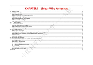
  • 57.   0 15 0 30 -10 45 These  are  shown  in  Figure  4.16  for  -20 60 h 2λ   and  5λ .  In  general,  the  total  -30 75 -40 number of lobes is equal to the integer that  -50 h=2 90 h=5 is closest to  -40 105 -30 2 120 number of lobes 1  -20 -10 135 0 150 180 165   2. Radiation power and directivity The total radiated power over the upper hemisphere of radius r using  / 1 ∙ | |   2 / | |                           (4‐101)  which simplifies, with the aid of (4‐99), to   
  • 58.                     (4‐102)   As  kh → ∞  the  radiated  power,  as  given  by  (4‐102),  is  equal  to  that  of  an  isolated element.     As  kh → 0, it can be shown that the power is twice that of an isolated element.  The radiation intensity can be written as    | |               (4‐103)                                  (4‐103)  The directivity can be written as    4                         (4‐104)  The maximum value occurs when  kh 2.881 h 0.4585 , and it is equal to  6.566  which  is  greater  than  four  times  that  of  an  isolated  element  (1.5).  The  pattern for  h 0.4585  is shown plotted in Figure 4.17 while the  directivity,  as  given by (4‐104), is displayed in Figure 4.18 for  0 h 5.   
  • 59.     Figure 4.17 Elevation plane amplitu ude pattern n of a vertica al infinitesim mal electric d dipole at a h height of  0.4585 ab bove an infin nite perfect electric connductor.  Us sing (4‐10 02), the radiation re esistance can be written as | | 2              (4‐105)                  (4‐19)  Th radiation  resista he  4.18  for 0 h ance  is  plotted  in  Figure  4 p 0 5  when  =  /50  5 an nd the element is ra adiating innto free‐s space (η  120).     
  • 60.     Figure 4.18 Directivity and radiation i D n n resistance of a vertical infinitesimal electric d dipole as a fu unction of  its height above an infinite perfectt electric conductor               
  • 61.   3. monopo ole In  prac ctice,  a  w wide  use  has  been made  o a  quar n  of  rter‐wavelength  m monopole  ( λ/4)  m mounted  above  a  g a ground  plane,  and fed  by  a coaxial  line,  as  s d  a  shown  in  Fig gure  4.199(a).  For  analysis  purposes a λ/4 image  is  introduc s,  ced  and  it  forms  the λ/2  eq quivalent  of  Figur 4.19(b).  It  should  be  e re  emphasize that  the  λ/2  ed  eqquivalent  of Figure 4.19(b) g gives the  correct field value es for the e actual sy ystem of  gure 4.19(a) only above the interface Fig e (z 0, 0 θ /2).         gure 4.19 Quarter‐ Fig ‐waveleng gth monopole on a an infinite perfect e electric co onductor     
  • 62.   Thus,  the  far‐zone  electric  and  magnetic  fields  for  the  λ/4  monopole  above  the ground plane are given, respectively, by (4‐84) and (4‐85).     ,            (4‐84, 4‐85)  The  input  impedance  of  a  λ/4  monopole  above  a  ground  plane  is  equal  to  one‐half  that  of  an  isolated  λ/2  dipole.  Thus,  referred  to  the  current  maximum,  the input impedance  Z   is given by  Z monopole Z dipole 73 j42.5 36.5 j21.25          (4‐106)               
  • 63.   4.7.4 Antennas for Mobile Communication Systems  The  dipole  and  monopole  are  two  of  the  most  widely  used  antennas  for  wireless mobile communication systems.     An  array  of  dipole  elements  is  extensively  used  as  an  antenna  at  the  base  station of a land mobile system while the monopole, because of its broadband  characteristics and simple construction, is perhaps to most common antenna  element  for  portable  equipment,  such  as  cellular  telephones,  cordless  telephones, automobiles, trains, etc.     An  alternative  to  the  monopole  for  the  handheld  unit  is  the  loop.  Other  elements include the inverted F, planar inverted F antenna (PIFA), microstrip  (patch), spiral, and others.  The variations of the input impedance, real and imaginary parts, of a vertical  monopole antenna mounted on an experimental unit are shown in Figure 4.21.     
  • 64.      
  • 65.     Figure 4.21    Input impedance, real and i imaginary parts, of a ve ertical mono opole mount ted on an  expe erimental ce hone device   ellular teleph e. It  is  a apparent  that  the  first  reso onance,  around  1,0 MHz,  is  slowly varying  000  y  values  of  immpedance versus frequency and  of desirable  magnitude,  for  practical  e  y,  f   
  • 66.   im mplementa ation.    Above the first t resonance, the im mpedance e is induct tive. The s second re esonance  rapid  changes  in  th values of  the  impedance.  These values  and  variation  of  he  s  e  im mpedance are usually undesirable for practical implementation.                  
  • 67.   4.7 7.5 Horizo ontal Elec ctric Dipo ole When the  line eleme n  ear  ent  is  placed ho orizontally y relative e to  the  infinitte  electric  grou und  plaane, as sh hown in Fiigure 4.24   4.    Fig gure 4.24 Ho orizontal eleectric dipole,, and its associated  imaage, above a an infinite, f flat, perfect nductor  t electric con The  aanalysis  p procedure of  this  is identica to  the  one  of  th vertica dipole.  e  s  al  he  al  Int troducing an  imag and  assuming  far  field  observat g  ge  a tions,  as  shown  in  Figure  4.2 25(a, b),         
  • 68.              (a) Horizontal electric c dipole abo ove ground p plane                 (b) Far‐ ‐field observ vations  gure 4.25 Ho Fig orizontal ele ectric dipole e above an infinite perfe ect electric conductor oefficient  is  equal  to  R Since  the  reflection  co 1,  The  direct  and  the  ref flect components c can be wr ritten as                   (4‐111)  ⟹             (4‐112)  ind  the  angle ψ ,  which  is  measu To  fi ured  from the  y‐ m  ‐axis  tow ward  the  ob bservation n point, w we first for rm   
  • 69.   ∙ ∙   (4‐113)  ⟹ 1 1                   (4‐114)  Since for far‐field observations        for phase variations            (4‐115a)              for  amplitude  variations            (4‐115b)  the total field, which is valid only above the ground plane (z≥h; 0≤θ≤/2, 0≤  ≤2), can be written as  E 1 sin sin 2 sin cos       (4‐116)  Equation (4‐116) again consists of the product of the field of a single isolated  element  placed  symmetrically  at  the  origin  and  a  factor  (within  the  brackets)  known as the array factor.