SlideShare ist ein Scribd-Unternehmen logo
1 von 10
Ch 6.5: Impulse Functions
In some applications, it is necessary to deal with phenomena
of an impulsive nature.
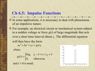
For example, an electrical circuit or mechanical system subject
to a sudden voltage or force g(t) of large magnitude that acts
over a short time interval about t0. The differential equation
will then have the form
small.is0and
otherwise,0
,big
)(
where
),(
00
>


 +<<−
=
=+′+′′
τ
ττ ttt
tg
tgcyybya
Measuring Impulse
In a mechanical system, where g(t) is a force, the total impulse
of this force is measured by the integral
Note that if g(t) has the form
then
In particular, if c = 1/(2τ), then I(τ) = 1 (independent of τ).
∫∫
+
−
∞
∞−
==
τ
τ
τ
0
0
)()()(
t
t
dttgdttgI


 +<<−
=
otherwise,0
,
)( 00 ττ tttc
tg
0,2)()()(
0
0
>=== ∫∫
+
−
∞
∞−
τττ
τ
τ
cdttgdttgI
t
t
Unit Impulse Function
Suppose the forcing function dτ(t) has the form
Then as we have seen, I(τ) = 1.
We are interested dτ(t) acting over
shorter and shorter time intervals
(i.e., τ → 0). See graph on right.
Note that dτ(t) gets taller and narrower
as τ → 0. Thus for t ≠ 0, we have


 <<−
=
otherwise,0
,21
)(
τττ
τ
t
td
1)(limand,0)(lim
00
==
→→
τ
τ
τ
τ
Itd
Dirac Delta Function
Thus for t ≠ 0, we have
The unit impulse function δ is defined to have the properties
The unit impulse function is an example of a generalized
function and is usually called the Dirac delta function.
In general, for a unit impulse at an arbitrary point t0,
1)(limand,0)(lim
00
==
→→
τ
τ
τ
τ
Itd
1)(and,0for0)( =≠= ∫
∞
∞−
dtttt δδ
1)(and,for0)( 000 =−≠=− ∫
∞
∞−
dttttttt δδ
Laplace Transform of δ (1 of 2)
The Laplace Transform of δ is defined by
and thus
{ } { } 0,)(lim)( 00
0
0 >−=−
→
tttdLttL τ
τ
δ
{ }
( ) ( )
[ ]
00
0
0
00
0
0
0
0
)cosh(
lim
)sinh(
lim
2
lim
2
1
lim
2
lim
2
1
lim)(lim)(
0
00
00
00
0
0
0
stst
st
ssst
tsts
t
t
st
t
t
stst
e
s
ss
e
s
s
e
ee
s
e
ee
ss
e
dtedtttdettL
−
→
−
→
−
−−
→
−−+−
→
+
−
−
→
+
−
−
→
∞
−
→
=





=






=




 −
=
+−=
−
=
=−=− ∫∫
τ
τ
τ
τ
ττ
τ
δ
τ
τ
ττ
τ
ττ
τ
τ
τ
τ
τ
ττ
τ
τ
Laplace Transform of δ (2 of 2)
Thus the Laplace Transform of δ is
For Laplace Transform of δ at t0= 0, take limit as follows:
For example, when t0= 10, we have L{δ(t-10)} = e-10s
.
{ } 0,)( 00
0
>=− −
tettL st
δ
{ } { } 1lim)(lim)( 0
00 0
0
0
==−= −
→→
st
t
ettdLtL
τ
τδ
Product of Continuous Functions and δ
The product of the delta function and a continuous function f
can be integrated, using the mean value theorem for integrals:
Thus
[ ]
)(
*)(lim
)*where(*)(2
2
1
lim
)(
2
1
lim
)()(lim)()(
0
0
00
0
0
0
0
0
0
0
tf
tf
ttttf
dttf
dttfttddttftt
t
t
=
=
+<<−=
=
−=−
→
→
+
−→
∞
∞−→
∞
∞−
∫
∫∫
τ
τ
τ
ττ
τ
τ
τττ
τ
τ
δ
)()()( 00 tfdttftt =−∫
∞
∞−
δ
Consider the solution to the initial value problem
Then
Letting Y(s) = L{y},
Substituting in the initial conditions, we obtain
or
)}7({}{2}{}{2 −=+′+′′ tLyLyLyL δ
[ ] [ ] s
esYyssYysysYs 72
)(2)0()()0(2)0(2)(2 −
=+−+′−−
Example 1: Initial Value Problem (1 of 3)
( ) s
esYss 72
)(22 −
=++
22
)( 2
7
++
=
−
ss
e
sY
s
0)0(,0)0(),7(22 =′=−=+′+′′ yytyyy δ
We have
The partial fraction expansion of Y(s) yields
and hence
Example 1: Solution (2 of 3)
22
)( 2
7
++
=
−
ss
e
sY
s
( ) 





++
=
−
16/154/1
4/15
152
)( 2
7
s
e
sY
s
( )
( )7
4
15
sin)(
152
1
)( 4/7
7 −= −−
tetuty t
With homogeneous initial conditions at t = 0 and no external
excitation until t = 7, there is no response on (0, 7).
The impulse at t = 7 produces a decaying oscillation that
persists indefinitely.
Response is continuous at t = 7 despite singularity in forcing
function. Since y' has a jump discontinuity at t = 7, y'' has an
infinite discontinuity there. Thus singularity in forcing
function is balanced by a corresponding singularity in y''.
Example 1: Solution Behavior (3 of 3)

Weitere ähnliche Inhalte

Was ist angesagt?

Torsion of circular shafts
Torsion of circular shaftsTorsion of circular shafts
Torsion of circular shaftsaero103
 
vibration of machines and structures
vibration of machines and structuresvibration of machines and structures
vibration of machines and structuresAniruddhsinh Barad
 
Laplace equation
Laplace equationLaplace equation
Laplace equationalexkhan129
 
6161103 4.8 resultants of a force and couple system
6161103 4.8 resultants of a force and couple system6161103 4.8 resultants of a force and couple system
6161103 4.8 resultants of a force and couple systemetcenterrbru
 
Causal Dynamical Triangulations
Causal Dynamical TriangulationsCausal Dynamical Triangulations
Causal Dynamical TriangulationsRene García
 
Travelling pulse through string
Travelling pulse through stringTravelling pulse through string
Travelling pulse through stringSunnie Tang
 
Inner outer and spectral factorizations
Inner outer and spectral factorizationsInner outer and spectral factorizations
Inner outer and spectral factorizationsSolo Hermelin
 
Mit2 092 f09_lec15
Mit2 092 f09_lec15Mit2 092 f09_lec15
Mit2 092 f09_lec15Rahman Hakim
 
Stability Result of Iterative procedure in normed space
Stability Result of Iterative procedure in normed spaceStability Result of Iterative procedure in normed space
Stability Result of Iterative procedure in normed spaceKomal Goyal
 
Differential calculus
Differential calculusDifferential calculus
Differential calculusChit Laplana
 
Applications of Differential Equations of First order and First Degree
Applications of Differential Equations of First order and First DegreeApplications of Differential Equations of First order and First Degree
Applications of Differential Equations of First order and First DegreeDheirya Joshi
 
Jawaban soal-latihan1mekanika
Jawaban soal-latihan1mekanikaJawaban soal-latihan1mekanika
Jawaban soal-latihan1mekanikamiranteogbonna
 
dESCRIPCION DEL PENDULO
dESCRIPCION DEL PENDULO dESCRIPCION DEL PENDULO
dESCRIPCION DEL PENDULO Rodrigo Gomez
 
Quantum phase estimation
Quantum phase estimationQuantum phase estimation
Quantum phase estimationtakumitano
 

Was ist angesagt? (20)

Torsion of circular shafts
Torsion of circular shaftsTorsion of circular shafts
Torsion of circular shafts
 
Unit5-KOM
Unit5-KOMUnit5-KOM
Unit5-KOM
 
vibration of machines and structures
vibration of machines and structuresvibration of machines and structures
vibration of machines and structures
 
Laplace equation
Laplace equationLaplace equation
Laplace equation
 
Ch02sol
Ch02solCh02sol
Ch02sol
 
6161103 4.8 resultants of a force and couple system
6161103 4.8 resultants of a force and couple system6161103 4.8 resultants of a force and couple system
6161103 4.8 resultants of a force and couple system
 
Causal Dynamical Triangulations
Causal Dynamical TriangulationsCausal Dynamical Triangulations
Causal Dynamical Triangulations
 
Travelling pulse through string
Travelling pulse through stringTravelling pulse through string
Travelling pulse through string
 
Inner outer and spectral factorizations
Inner outer and spectral factorizationsInner outer and spectral factorizations
Inner outer and spectral factorizations
 
Mit2 092 f09_lec15
Mit2 092 f09_lec15Mit2 092 f09_lec15
Mit2 092 f09_lec15
 
Stability Result of Iterative procedure in normed space
Stability Result of Iterative procedure in normed spaceStability Result of Iterative procedure in normed space
Stability Result of Iterative procedure in normed space
 
Differential calculus
Differential calculusDifferential calculus
Differential calculus
 
Applications of Differential Equations of First order and First Degree
Applications of Differential Equations of First order and First DegreeApplications of Differential Equations of First order and First Degree
Applications of Differential Equations of First order and First Degree
 
Jawaban soal-latihan1mekanika
Jawaban soal-latihan1mekanikaJawaban soal-latihan1mekanika
Jawaban soal-latihan1mekanika
 
dESCRIPCION DEL PENDULO
dESCRIPCION DEL PENDULO dESCRIPCION DEL PENDULO
dESCRIPCION DEL PENDULO
 
Simple harmonic motion1
Simple harmonic motion1Simple harmonic motion1
Simple harmonic motion1
 
Quantum phase estimation
Quantum phase estimationQuantum phase estimation
Quantum phase estimation
 
P13 054
P13 054P13 054
P13 054
 
Cycloidal pendulum
Cycloidal pendulumCycloidal pendulum
Cycloidal pendulum
 
Sol67
Sol67Sol67
Sol67
 

Andere mochten auch

Chemical &amp; Microbial analysis of farm &amp; forest soil
Chemical &amp; Microbial analysis of farm &amp; forest soilChemical &amp; Microbial analysis of farm &amp; forest soil
Chemical &amp; Microbial analysis of farm &amp; forest soilIshan Trivedi
 
Applications of matrices in real life
Applications of matrices in real lifeApplications of matrices in real life
Applications of matrices in real lifeSuhaibFaiz
 
Eigen value and eigen vector
Eigen value and eigen vectorEigen value and eigen vector
Eigen value and eigen vectorRutvij Patel
 
presentation on matrix
 presentation on matrix presentation on matrix
presentation on matrixNikhi Jain
 
Matrices And Application Of Matrices
Matrices And Application Of MatricesMatrices And Application Of Matrices
Matrices And Application Of Matricesmailrenuka
 

Andere mochten auch (7)

Ch07 2
Ch07 2Ch07 2
Ch07 2
 
Chemical &amp; Microbial analysis of farm &amp; forest soil
Chemical &amp; Microbial analysis of farm &amp; forest soilChemical &amp; Microbial analysis of farm &amp; forest soil
Chemical &amp; Microbial analysis of farm &amp; forest soil
 
Applications of matrices in real life
Applications of matrices in real lifeApplications of matrices in real life
Applications of matrices in real life
 
Eigen value and eigen vector
Eigen value and eigen vectorEigen value and eigen vector
Eigen value and eigen vector
 
Application of matrices in real life
Application of matrices in real lifeApplication of matrices in real life
Application of matrices in real life
 
presentation on matrix
 presentation on matrix presentation on matrix
presentation on matrix
 
Matrices And Application Of Matrices
Matrices And Application Of MatricesMatrices And Application Of Matrices
Matrices And Application Of Matrices
 

Ähnlich wie Ch06 5

Circuit Network Analysis - [Chapter4] Laplace Transform
Circuit Network Analysis - [Chapter4] Laplace TransformCircuit Network Analysis - [Chapter4] Laplace Transform
Circuit Network Analysis - [Chapter4] Laplace TransformSimen Li
 
Julio Bravo's Master Graduation Project
Julio Bravo's Master Graduation ProjectJulio Bravo's Master Graduation Project
Julio Bravo's Master Graduation ProjectJulio Bravo
 
The finite time turnpike phenomenon for optimal control problems
The finite time turnpike phenomenon for optimal control problemsThe finite time turnpike phenomenon for optimal control problems
The finite time turnpike phenomenon for optimal control problemsMartinGugat
 
Lec 05(actuator sizing).pdf
Lec 05(actuator sizing).pdfLec 05(actuator sizing).pdf
Lec 05(actuator sizing).pdfMohamed Atef
 
Lecture5 Signal and Systems
Lecture5 Signal and SystemsLecture5 Signal and Systems
Lecture5 Signal and Systemsbabak danyal
 
Material modelling for design
Material modelling for design Material modelling for design
Material modelling for design Er Shambhu Chauhan
 
Optimal debt maturity management
Optimal debt maturity managementOptimal debt maturity management
Optimal debt maturity managementADEMU_Project
 
MATLAB sessions Laboratory 6MAT 275 Laboratory 6Forced .docx
MATLAB sessions Laboratory 6MAT 275 Laboratory 6Forced .docxMATLAB sessions Laboratory 6MAT 275 Laboratory 6Forced .docx
MATLAB sessions Laboratory 6MAT 275 Laboratory 6Forced .docxandreecapon
 
lecture 5 courseII (6).pptx
lecture 5 courseII (6).pptxlecture 5 courseII (6).pptx
lecture 5 courseII (6).pptxAYMENGOODKid
 
optimal solution method of integro-differential equaitions under laplace tran...
optimal solution method of integro-differential equaitions under laplace tran...optimal solution method of integro-differential equaitions under laplace tran...
optimal solution method of integro-differential equaitions under laplace tran...INFOGAIN PUBLICATION
 
Notes mech v
Notes mech vNotes mech v
Notes mech vRung Heo
 
Controllability of Linear Dynamical System
Controllability of  Linear Dynamical SystemControllability of  Linear Dynamical System
Controllability of Linear Dynamical SystemPurnima Pandit
 
Convolution representation impulse response
Convolution representation impulse responseConvolution representation impulse response
Convolution representation impulse responseuradiraghu92
 

Ähnlich wie Ch06 5 (20)

Circuit Network Analysis - [Chapter4] Laplace Transform
Circuit Network Analysis - [Chapter4] Laplace TransformCircuit Network Analysis - [Chapter4] Laplace Transform
Circuit Network Analysis - [Chapter4] Laplace Transform
 
Sol67
Sol67Sol67
Sol67
 
Ch03 9
Ch03 9Ch03 9
Ch03 9
 
Julio Bravo's Master Graduation Project
Julio Bravo's Master Graduation ProjectJulio Bravo's Master Graduation Project
Julio Bravo's Master Graduation Project
 
residue
residueresidue
residue
 
The finite time turnpike phenomenon for optimal control problems
The finite time turnpike phenomenon for optimal control problemsThe finite time turnpike phenomenon for optimal control problems
The finite time turnpike phenomenon for optimal control problems
 
Chapter3 laplace
Chapter3 laplaceChapter3 laplace
Chapter3 laplace
 
Lec 05(actuator sizing).pdf
Lec 05(actuator sizing).pdfLec 05(actuator sizing).pdf
Lec 05(actuator sizing).pdf
 
Lecture5 Signal and Systems
Lecture5 Signal and SystemsLecture5 Signal and Systems
Lecture5 Signal and Systems
 
Material modelling for design
Material modelling for design Material modelling for design
Material modelling for design
 
Optimal debt maturity management
Optimal debt maturity managementOptimal debt maturity management
Optimal debt maturity management
 
MATLAB sessions Laboratory 6MAT 275 Laboratory 6Forced .docx
MATLAB sessions Laboratory 6MAT 275 Laboratory 6Forced .docxMATLAB sessions Laboratory 6MAT 275 Laboratory 6Forced .docx
MATLAB sessions Laboratory 6MAT 275 Laboratory 6Forced .docx
 
lecture 5 courseII (6).pptx
lecture 5 courseII (6).pptxlecture 5 courseII (6).pptx
lecture 5 courseII (6).pptx
 
optimal solution method of integro-differential equaitions under laplace tran...
optimal solution method of integro-differential equaitions under laplace tran...optimal solution method of integro-differential equaitions under laplace tran...
optimal solution method of integro-differential equaitions under laplace tran...
 
Notes mech v
Notes mech vNotes mech v
Notes mech v
 
Lecture 5: The Convolution Sum
Lecture 5: The Convolution SumLecture 5: The Convolution Sum
Lecture 5: The Convolution Sum
 
Analytic dynamics
Analytic dynamicsAnalytic dynamics
Analytic dynamics
 
Controllability of Linear Dynamical System
Controllability of  Linear Dynamical SystemControllability of  Linear Dynamical System
Controllability of Linear Dynamical System
 
Solution a ph o 3
Solution a ph o 3Solution a ph o 3
Solution a ph o 3
 
Convolution representation impulse response
Convolution representation impulse responseConvolution representation impulse response
Convolution representation impulse response
 

Mehr von Rendy Robert (20)

Ch08 3
Ch08 3Ch08 3
Ch08 3
 
Ch08 1
Ch08 1Ch08 1
Ch08 1
 
Ch07 9
Ch07 9Ch07 9
Ch07 9
 
Ch07 8
Ch07 8Ch07 8
Ch07 8
 
Ch07 7
Ch07 7Ch07 7
Ch07 7
 
Ch07 6
Ch07 6Ch07 6
Ch07 6
 
Ch07 5
Ch07 5Ch07 5
Ch07 5
 
Ch07 4
Ch07 4Ch07 4
Ch07 4
 
Ch07 3
Ch07 3Ch07 3
Ch07 3
 
Ch07 1
Ch07 1Ch07 1
Ch07 1
 
Ch06 6
Ch06 6Ch06 6
Ch06 6
 
Ch06 3
Ch06 3Ch06 3
Ch06 3
 
Ch06 2
Ch06 2Ch06 2
Ch06 2
 
Ch05 8
Ch05 8Ch05 8
Ch05 8
 
Ch05 7
Ch05 7Ch05 7
Ch05 7
 
Ch05 6
Ch05 6Ch05 6
Ch05 6
 
Ch05 5
Ch05 5Ch05 5
Ch05 5
 
Ch05 4
Ch05 4Ch05 4
Ch05 4
 
Ch05 3
Ch05 3Ch05 3
Ch05 3
 
Ch05 2
Ch05 2Ch05 2
Ch05 2
 

Ch06 5

  • 1. Ch 6.5: Impulse Functions In some applications, it is necessary to deal with phenomena of an impulsive nature. For example, an electrical circuit or mechanical system subject to a sudden voltage or force g(t) of large magnitude that acts over a short time interval about t0. The differential equation will then have the form small.is0and otherwise,0 ,big )( where ),( 00 >    +<<− = =+′+′′ τ ττ ttt tg tgcyybya
  • 2. Measuring Impulse In a mechanical system, where g(t) is a force, the total impulse of this force is measured by the integral Note that if g(t) has the form then In particular, if c = 1/(2τ), then I(τ) = 1 (independent of τ). ∫∫ + − ∞ ∞− == τ τ τ 0 0 )()()( t t dttgdttgI    +<<− = otherwise,0 , )( 00 ττ tttc tg 0,2)()()( 0 0 >=== ∫∫ + − ∞ ∞− τττ τ τ cdttgdttgI t t
  • 3. Unit Impulse Function Suppose the forcing function dτ(t) has the form Then as we have seen, I(τ) = 1. We are interested dτ(t) acting over shorter and shorter time intervals (i.e., τ → 0). See graph on right. Note that dτ(t) gets taller and narrower as τ → 0. Thus for t ≠ 0, we have    <<− = otherwise,0 ,21 )( τττ τ t td 1)(limand,0)(lim 00 == →→ τ τ τ τ Itd
  • 4. Dirac Delta Function Thus for t ≠ 0, we have The unit impulse function δ is defined to have the properties The unit impulse function is an example of a generalized function and is usually called the Dirac delta function. In general, for a unit impulse at an arbitrary point t0, 1)(limand,0)(lim 00 == →→ τ τ τ τ Itd 1)(and,0for0)( =≠= ∫ ∞ ∞− dtttt δδ 1)(and,for0)( 000 =−≠=− ∫ ∞ ∞− dttttttt δδ
  • 5. Laplace Transform of δ (1 of 2) The Laplace Transform of δ is defined by and thus { } { } 0,)(lim)( 00 0 0 >−=− → tttdLttL τ τ δ { } ( ) ( ) [ ] 00 0 0 00 0 0 0 0 )cosh( lim )sinh( lim 2 lim 2 1 lim 2 lim 2 1 lim)(lim)( 0 00 00 00 0 0 0 stst st ssst tsts t t st t t stst e s ss e s s e ee s e ee ss e dtedtttdettL − → − → − −− → −−+− → + − − → + − − → ∞ − → =      =       =      − = +−= − = =−=− ∫∫ τ τ τ τ ττ τ δ τ τ ττ τ ττ τ τ τ τ τ ττ τ τ
  • 6. Laplace Transform of δ (2 of 2) Thus the Laplace Transform of δ is For Laplace Transform of δ at t0= 0, take limit as follows: For example, when t0= 10, we have L{δ(t-10)} = e-10s . { } 0,)( 00 0 >=− − tettL st δ { } { } 1lim)(lim)( 0 00 0 0 0 ==−= − →→ st t ettdLtL τ τδ
  • 7. Product of Continuous Functions and δ The product of the delta function and a continuous function f can be integrated, using the mean value theorem for integrals: Thus [ ] )( *)(lim )*where(*)(2 2 1 lim )( 2 1 lim )()(lim)()( 0 0 00 0 0 0 0 0 0 0 tf tf ttttf dttf dttfttddttftt t t = = +<<−= = −=− → → + −→ ∞ ∞−→ ∞ ∞− ∫ ∫∫ τ τ τ ττ τ τ τττ τ τ δ )()()( 00 tfdttftt =−∫ ∞ ∞− δ
  • 8. Consider the solution to the initial value problem Then Letting Y(s) = L{y}, Substituting in the initial conditions, we obtain or )}7({}{2}{}{2 −=+′+′′ tLyLyLyL δ [ ] [ ] s esYyssYysysYs 72 )(2)0()()0(2)0(2)(2 − =+−+′−− Example 1: Initial Value Problem (1 of 3) ( ) s esYss 72 )(22 − =++ 22 )( 2 7 ++ = − ss e sY s 0)0(,0)0(),7(22 =′=−=+′+′′ yytyyy δ
  • 9. We have The partial fraction expansion of Y(s) yields and hence Example 1: Solution (2 of 3) 22 )( 2 7 ++ = − ss e sY s ( )       ++ = − 16/154/1 4/15 152 )( 2 7 s e sY s ( ) ( )7 4 15 sin)( 152 1 )( 4/7 7 −= −− tetuty t
  • 10. With homogeneous initial conditions at t = 0 and no external excitation until t = 7, there is no response on (0, 7). The impulse at t = 7 produces a decaying oscillation that persists indefinitely. Response is continuous at t = 7 despite singularity in forcing function. Since y' has a jump discontinuity at t = 7, y'' has an infinite discontinuity there. Thus singularity in forcing function is balanced by a corresponding singularity in y''. Example 1: Solution Behavior (3 of 3)