The document compares economic base models and input-output models. Economic base models analyze multiplier effects at the basic/non-basic sector level, while input-output models analyze impacts at a more precise sector-by-sector level by tracing dollar flows between industries. Input-output models build upon economic base models by accounting for inter-industry transactions and better capturing complex interdependencies between sectors.

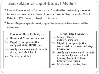
1. Econ Base vs Input-Output Models
 Leontief developed an “input-output” method for estimating economic
impacts and tracing the flows of dollars. Leontief later won the Nobel
Prize in 1973, largely related to this work.
 Input-Output expands heavily upon the economic base model of the
economy.
Economic Base Techniques Input-Output Analysis
1) Basic and Non-basic sectors 1) Many different
industries/sectors
2) Ripple (multiplier) effects 2) Ripple (multiplier) effects
analyzed at the B/NB level contained in the interindustry
3) Analyzes changes and impacts transactions
at a gross B/NB level 3) Analyzes changes and impacts
4) Very general, but… at a sector by sector level,
tracing flows of dollars
between industries
4) Much more precise, but…

2. The Economic Base Theoretical Model
• The EB model assumes that the basic sector is the primary
cause of local economic growth; that is, it is the economic
base of the local economy.
Non-Local
$$$’s
Local
$$$’s
Basic Sector Non-Basic Sector
Employment Employment
The Local Economy

3. Input-Output Model
The IO model is centered on the idea of inter-industry
transactions:
Industries use the products of other industries to produce their
own products.
For example - automobile producers use steel, glass, rubber,
and plastic products to produce automobiles.
Outputs from one industry become inputs to another.
When you buy a car, you affect the demand for glass, plastic,
steel, etc.
Taken from a Power Point presentation prepared by
Pam Perlich at the University of Utah.
http://www.business.utah.edu/~bebrpsp/IO/IO.ppt

4. Basic Input-Output Logic
Tires
Glass Plastic Other
Steel
Components
Automobile Factory

5. From the Tire Individual
Consumers
Producer’s
Perspective FINAL
School
Districts DEMAND
FOR TIRES
Tire Factory Trucking
Companies
INTER-
Automobile
MEDIATE
Factory DEMAND
FOR
TIRES

6. Input-Output Analysis: The BIG Point
• The implicit assumption in economic base techniques is that each basic
sector job has a multiplier (or ripple) effect on the wider economy because
of purchases of non-basic goods and services to support the basic
production activity. (the Basic Sector drives the Non-basic Sector)
• However, we know that Non-basic sector businesses purchase Non-basic
goods and services and Basic sector businesses purchase Basic sector goods
and services. There are inter-industry linkages not contained within the
Economic Base model. The economy is much more complex than the
economic base techniques allow or attempt to model.
• The central advantage of Input-Output analysis is that it tries to estimate
these inter-industry transactions and use those figures to estimate the
economic impacts of any changes to the economy.
• Instead of assuming a change in a basic sector industry having a generalized
multiplier effect, the IO approach estimates how many goods and services
from other sectors are needed (inputs) to produce each dollar of output for
the sector in question. Therefore it is possible to do a much more precise
calculation of the economic impacts of a given change to the economy.

7. IO Conceptualization of the Economy
• The major conceptual step is to divide the economy into “purchasers”
and “suppliers”.
--Primary Suppliers: They sell primary inputs (labor, raw materials) to
other industries. Payments to these suppliers are “primary inputs”
because they generate no further sales. (example: Households)
--Intermediate Suppliers: They purchase inputs for processing into outputs
they supply to other firms or to final purchasers. (example: Automaker)
--Intermediate Purchasers: They purchase outputs of suppliers for use as
inputs for further processing. (example: Automaker)
--Final Purchasers: Purchase the outputs of suppliers in their final form
and for final use. (example: Households)
• Intermediate Suppliers and Intermediate Purchasers are the same thing!
• Primary Suppliers and Final Purchasers may or may not be the same
entities. When they are the same (households), these activities are
understood as separate activities.

8. Simplified Circular Flow View of The
Economy
$$ Consumption Spending (Yi)
Goods & Services
Households Businesses Businesses
Labor
$$ Wages & Salaries Businesses purchase from
other businesses to produce
Households buy Households sell
their own goods / services.
the output of labor & other
business: final inputs to business This is intermediate
as inputs to demand or xij (output of
demand or Yi
production industry i sold to industry j)
Taken from a Power Point presentation
prepared by Pam Perlich at the University of Utah.
http://www.business.utah.edu/~bebrpsp/IO/IO.ppt

9. The Structure of IO Analysis
• The ultimate goal of the Input-Output Analysis technique is to
generate a Total Requirements Table that shows the flows of dollars
between industries in the production of output for a given sector.
• To arrive at this final result, IO Analysis requires two earlier steps:
1) Transactions table: Contains basic data on the flows of goods and
services among suppliers and purchasers during a study year.
2) Direct requirements table: Derived from the transactions table,
this shows the inputs required directly from different suppliers by
each intermediate purchaser for each unit of output that purchaser
produces.
• “Input output analysis can be thought of as documenting and
exploring the precise systems of interindustry exchange through
which different components of regional product become different
components of regional income.” (Bendavid-Val, p. 87-88)
• Let’s review Bendavid-Val’s “Islandia example”.

10. The Transaction Table and Direct Reqs Tables
The Transactions Table
(in thousands of units)
Intermediate Purchasers Final Purchasers Total
--Agriculture --Manufacturing --Households Sales (outputs)
Intermediate Suppliers
--Agriculture 10 30 60 100
--Manufacturing 5 10 35 50
Primary Suppliers
--Households 85 10 15 110
Total Purchases (inputs) 100 50 110 260
Direct Requirements Table
(in thousands of units)
Purchasers
--Agriculture --Manufacturing
Intermediate Suppliers Every unit of output
--Agriculture 0.10 0.60 requires inputs of a certain
--Manufacturing 0.05 0.20 amount from other areas
Primary Suppliers of the economy.
--Households 0.85 0.20
Total Purchases (inputs) 1.00 1.00

11. The First Round of Economic Impacts
Direct Requirements Table
(in thousands of units)
Intermediate Purchasers
--Agriculture --Manu
Intermediate Suppliers
--Agriculture 0.10 0.60
--Manufacturing 0.05 0.20
Primary Suppliers
--Households 0.85 0.20
Total Purchases (inputs) 1.00 1.00
Total Requirements Calculation (First Round)
(in thousands of units)
Sales to Sales as Direct Inputs
Final Purch. To Agr To Manu Total
By Agriculture 200 20 60 80 To
By Manufacturing 100 10 20 30 Rd. 2
By Households 0 170 20 190
Total indirect rounds
By All Supliers 300 300

12. The Second-Fourth Rounds of Econ. Impacts
Total Requirements Calculation (Second Round)
(in thousands of units)
Sales to Sales as Direct Inputs
Final Purch. To Agr To Manu Total
By Agriculture 80 8.0 18.0 26.0
By Manufacturing 30 4.0 6.0 10.0
By Households 0 68.0 6.0 74.0
Total indirect rounds 110.0
Total Requirements Calculation (Third Round)
(in thousands of units)
Sales to Sales as Direct Inputs
Final Purch. To Agr To Manu Total
By Agriculture 26 2.6 6.0 8.6
By Manufacturing 10 1.3 2.0 3.3
By Households 0 22.1 2.0 24.1
Total indirect rounds 36.0
Total Requirements Calculation (Fourth Round)
(in thousands of units)
Sales to Sales as Direct Inputs
Final Purch. To Agr To Manu Total
By Agriculture 8.6 0.9 2.0 2.8 and so on
By Manufacturing 3.3 0.4 0.7 1.1 until the mult.
By Households 0 7.3 0.7 8.0 effect ends
Total indirect rounds 11.9

13. The Total Requirements Results
Total Direct and Indirect Requirements Calculation
(in thousands of units)
Sales to Final Total Total Total
Purchasers Direct Sales Indirect Sales Sales
Agriculture 200.0 80.0 38.7 318.7
Manufacturing 100.0 30.0 14.9 144.9
Households -- 190.0 109.6 299.6
Total 300.0 300.0 163.1 763.1
When:
1) there are “Final Sales” of Agriculture = 200 and “Final Sales” of
Manufacturing = 100
2) we see a Total Economic Impact = 763.1, with that impact broken
down as:
1) 300.0 in Initial Sales to Final Purchasers
2) 300.0 in Total Direct Sales
3) 163.1 in Total Indirect Sales
The 300 units in Final Sales generate an additional 463.1 units of
economic activity. This illustrates the multiplier effect captured by
IO models.

14. The Total Requirements Table
Total Requirements Table
Every Unit in Final Demand of…
Requires Total Sales by Agriculture Manufacturing
Agriculture 1.15 0.86
Manufacturing 0.07 1.29
Households 1.00 1.00
Total 2.22 3.15
For Agriculture 1.00 Sales to Final Purchasers
1.00 Sales by Primary Suppliers
0.22 Interindustry transactions
Similar to our Base Multiplier in Econ Base Theory
A 1.0 unit increase in demand for agriculture leads to
a total of 2.22 of sales.
For Manufacturing 1.00 Sales to Final Purchasers
1.00 Sales by Primary Suppliers
1.15 Interindustry transactions
Similar to our Base Multiplier in Econ Base Theory
A 1.0 unit increase in demand for manufacturing leads to
a total of 3.15 of sales.

15. RIMS Multipliers
• The Bureau of Economic Analysis (BEA) produces State Level
Regional Input-Output Multipliers by industrial sector which are often
used as the basis for constructing an IO model.
• Originally developed in the 1970s, RIMS (Regional Industrial
Multiplier System) multipliers are used for “impact analysis” for a
given economy.
• RIMS II data were developed in the 1980’s (latest version is 1998)
• Users can purchase data from BEA for $275 per region. BEA provides
handbooks for the use of this data.
• County or multi-county regional RIMS data come in two series
Series I: for 490 detailed industries
Series II: for 38 industry aggregations
• Empirical analysis shows that RIMS II data is accurate within 5% of
locally developed industry multipliers.
• Advantages of the RIMS Multipliers:
1) Cheap 2) Can be compared across regions
3) Detailed industries 4) Updated regularly to reflect new data

16. Example RIMS Multipliers
1
Total dollar impact due to $1 in output in the industry. 2Change in earnings due to $1 change in
industry. 3Change in employment resulting from $1 million increase in output delivered to final demand.

17. For More Info on RIMS Multipliers
• The Bureau of Economic Analysis (BEA) has several web
resources on RIMS Multipliers and how they are prepared:
RIMSII Home Page
http://www.bea.doc.gov/bea/regional/rims/
Brief Description of RIMS II
http://www.bea.doc.gov/bea/regional/rims/brfdesc.cfm
RIMSII User’s Handbook
http://www.bea.doc.gov/bea/ARTICLES/REGIONAL/PERSINC/M
eth/rims2.pdf

18. The Problems with IO Analysis
Practical Issues
• Data needs and complexity: IO models are tremendously complex and very
data hungry. This typically places these models in the hands of experts.
Theoretical Issues
• Time/Data issues: Usually a single year’s data are used to develop the
Total Requirements Table. But 1) purchases may actually reflect a longer
term investment and 2) short term trends may impact the data.
• Stability of the technical coefficients over time: Technology changes,
prices change, and demand changes, all affecting the coefficients in the Tot
Reqs Table. This can impact the results if the coefficients are “out of date”.
• IO assumes a linear relationship between increasing demand for inputs
and outputs: This assumes away 1) externalities and 2) increasing/
decreasing returns to scale.
• Industrial categorization: IO models still assume that each industry 1) has
a single, homogeneous production function and 2) each produces one
product. These assumptions do not reflect the real economy very well.

19. The Power of IO Models
• Despite these problems IO analysis is a tremendously popular and
powerful analytical tool.
• “The chief value of regional input-output analysis is in its descriptive
analytical power.” (Bendavid-Val, p.113)
• “As a descriptive tool, input-output tables:
-present an enormous quantity of information in a concise, orderly,
and easily understood fashion;
-provide a comprehensive picture of the interindustry structure of
the regional economy;
-point up the strategic importance of various industries and sectors;
-highlight possible opportunities for strengthening regional income
and employment multiplication.” (Bendavid-Val, p.113)
• Urban Planners should be capable of understanding the structure,
assumptions, and data requirements of Input-Output Analysis. While
you may not be performing this analysis in your jobs, you almost
certainly will come across this type of work sometime in your career.