The document discusses different methods for sampling vegetation, including quadrats, transects, and sampling systems. It describes the different types of quadrats - plain, cover, and point - and how transects can be used in the form of line, belt, and interval transects. Random sampling is presented as an objective technique but limitations are discussed. The number of quadrats needed is calculated based on variability between samples. Different attributes that can be measured are also outlined, including density, cover, and abundance.

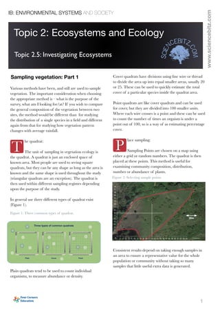
1.
1
IB: ENVIRONMENTAL SYSTEMS AND SOCIETY
Various methods have been, and still are used to sample
vegetation. The important consideration when choosing
the appropriate method is – what is the purpose of the
survey, what am I looking for/at? If you wish to compare
the general composition of the vegetation between two
sites, the method would be different than for studying
the distribution of a single species in a
fi
eld and different
again from that for studying how vegetation pattern
changes with average rainfall.
T
he quadrat:
The unit of sampling in vegetation ecology is
the quadrat. A quadrat is just an enclosed space of
known area. Most people are used to seeing square
quadrats, but they can be any shape as long as the area is
known and the same shape is used throughout the study
(triangular quadrats are an exception). The quadrat is
then used within different sampling regimes depending
upon the purpose of the study.
In general use three different types of quadrat exist
(Figure 1).
Plain quadrats tend to be used to count individual
organisms, to measure abundance or density.
Cover quadrats have divisions using
fi
ne wire or thread
to divide the area up into equal smaller areas, usually 20
or 25. These can be used to quickly estimate the total
cover of a particular species inside the quadrat area.
Point quadrats are like cover quadrats and can be used
for cover, but they are divided into 100 smaller units.
Where each wire crosses is a point and these can be used
to count the number of times an orgaism is under a
point out of 100, so is a way of as estimating percentage
cover.
P
lace sampling:
Sampling Points are chosen on a map using
either a grid or random numbers. The quadrat is then
placed at these points. This method is useful for
examining community composition, distribution,
number or abundance of plants.
Consistent results depend on taking enough samples in
an area to ensure a representative value for the whole
population or community without taking so many
samples that little useful extra data is generated.
Sampling vegetation: Part 1
Topic 2: Ecosystems and Ecology
Topic 2.5: Investigating Ecosystems
www.sciencebitz.com
Figure 1: Three common types of quadrat.
Figure 2: Selecting sample points

2.
2
T
he Transect
A transect is a sampling line either through a
single habitat or area, or through various habitats.
Line Transects
In its simplest form all plants that touch the transect
line are counted in the sample, though more often the
species that touch the transect at set regular intervals of
say 1 or 5 m are counted along very long transects.
While this may not intuitively seem to have any
relationship to a quadrat, the line of the transect is in
effect just a very long narrow rectangle.
Belt Transects
If this idea is expanded on, all the plants occurring a
set distance either side of the transect line can be
included in a count. This method has been used to
examine the patterns of seed dispersal from parent
trees in a forest for instance, by surveying the frequency
of saplings away from the base of a tree in different
directions.
A belt transect is much easier to think of as a very long
narrow quadrat.
Interval Transects
Quadrats can be used in conjunction with a line
transect and placed at regular intervals. This method is
useful if the transect runs along an environmental
gradient such as altitude or salinity for example. Used
this way the samples can help to show how biotic
composition can change with abiotic variation.
Interval transects are especially useful where an
environmental gradient is suspected to be in
fl
uencing
distribution.
IB: ENVIRONMENTAL SYSTEMS AND SOCIETY
www.sciencebitz.com
Figure 3: A Line Transect.
Line Transect
Transect Sample Boundary
Transect Sample Boundary
Figure 4: A Belt Transect.
Line Transect
Quadrats placed at equal intervals
Figure 5: Interval Transect.
Thinking points to discuss with students:
What are the bene
fi
ts and problems with
each of the three transect methods?

3.
3
S
ampling systems
The quadrat is the basic unit most often used
to sample vegetation.
Using quadrats:
There are some rules that need to be thought about
before using quadrats for any sampling exercise
1. The area of the quadrat must be known
2. Enough quadrat samples need to be taken to be
representative of the whole population or habitat
3. The populations counted in the quadrat must be
known exactly: it must be possible to distinguish
individual species (this is different to knowing the
name of a species)
4. The quadrat size must be suitable for the plant
counted: 1m2 for grasslands – 50m2 for tree canopy
species
5. The quadrats must be representative of the whole
area. This is usually achieved by using random
sampling though importantly this is an assumption
and often not the reality
Random sampling
Often random sampling is presented as almost an
answer to everything. However as with all sampling
and survey techniques random sampling has its bene
fi
ts
and disadvantages.
The strongest case for random camping is that it
removes operator bias when choosing what to sample.
When planned and well executed this may indeed be
true, but that is not always the case as will be discussed
later.
Methodology
You
fi
rst need to select your sample area. If any
questions (the RQ) are being asked about reasons for
distribution then the area being sampled should contain
a fairly homogeneous vegetation type. This will help
reduce other variables that may have an impact at a
consistent level but it may not eliminate them entirely.
i.e: The distribution of common stinging nettle (Urtica
Doioica) in Europe is strongly associated with nutrient
enrichment. However where Dogs mercury (Mercurialis
perennis) exists in limestone woodlands the distribution
of stinging nettle is inhibited by competition for
phosphates (Jefferson) even where the nutrient is
abundant. So sampling an aren of vegetation that
contains both open woodland and closed woodland to
ask any questions about how the distribution of stinging
nettles is related to Nitrogen enrichment may not yield
any meaningful answers if the closed woodland also
contains Dogs mercury.
Figure 2 below and above illustrates an area of
vegetation that has been mapped out to concentrate on
a fairly homogeneous stand of grazed rough pasture.
The surrounding areas of developing scrub has been
excluded.
Using a random number grid or a random number
generator, two coordinates are created and the
quadrant placed at the intersect of these coordinates.
This process is repeated for the total number of sample
points required for the survey. Traditionally, selection of
sample points will have been conducted using large
scale maps, surveyors tapes and marking lines. However
where GPS reception is good pre-plotting coordinates
on mapping software and using a smart phone to locate
them in the
fi
eld is an ef
fi
cient way of working.
IB: ENVIRONMENTAL SYSTEMS AND SOCIETY
www.sciencebitz.com
Figure 2: Selecting sample points
Figure 6: Quadrat placed at a sample point

4.
4
L
imitations of Random Sampling
Random sampling is classi
fi
ed as an objective
survey technique.
This does not mean that random sampling is without its
problems.
Things to think about?
1. How random is the sample in reality? If a random
number grid is used and the sample coordinates
selected by using a pin and closing your eyes, there
is a tendency that numbers nearer the centre of the
grid are chosen rather than those at the edges. As
long as the possible numbers in the grid are
repeated randomly enough then this should not be
a problem, however some grids are not extensive
enough to guarantee this.
2. Possibly the biggest problem with random sampling
regimes is that they may miss species that are less
represented in the vegetation. Rare species tend to
be under counted. This may not be important if
you are sampling a single species that is quite
common, but for community surveys and those
interested in rarer species it may be.
3. Edge effect. Because of the nature of using
coordinates - the edges of any regular shaped area
tend to be sampled less than areas towards the
middle. A solution to this is dividing the whole
sample area into blocks and taking equal random
samples inside each block. Nested samples (Figure
7).
4. By their very nature different species display
different distribution patterns. Random, Clumped
or Uniform (Figure 8). Where species are clumped
together in patches
random sampling
runs the chance of
under sampling the
population in any
habitat, so care
needs to be taken to
ensure that enough
sample points are
used to effectively
sample the
population. Again
nested designs help
to alleviate this
problem.
If a survey is designed to
understand an attribute
of a single species, then
time taken to develop a
good understanding of
that species is time well
spent. That often does
not require resorting to
extensive literature searches. Observing the species in
the field can yield a lot of valuable understanding about
the species in question prior to considering an
appropriate survey regime.
S
ubjective v Objective Survey techniques
There is a wealth of good advice in the
literature about the benefits of either and
numerous different methodologies that will lead to
collection of sound usable data in the correct
conditions. Below are a few thought points about each.
Subjective sampling
Sample sites are consciously chosen as representative of
predetermined vegetation classes.
Most flexible sampling scheme
Allows for experience and decision making ability of
the investigator
Best used in areas where there are clear boundaries
between plant communities
Good approach for vegetation classification
Objective sampling
Sample sites are chosen according to chance (i.e.
random sampling) or system
IB: ENVIRONMENTAL SYSTEMS AND SOCIETY
www.sciencebitz.com
Figure 7: Nested Random sampling regime
Random distribution
Clumped distribution
Uniform distribution
Figure 8: Distribution
patterns

5.
5
Essential if probability statistics are to be used to back
up the conclusions (may be as not all statistics are
probability based)
Especially where the objective is to determine the
causes of variation within a single plant community
Can be used in areas where boundaries between
communities are indistinct for wider surveys
Can be a good approach for where environmental
gradients may be at work - with a thoughtful regime.
NB* The overall sampling regime for a particular use
can apply a mix of both subjective and objective
components. Sample sites may be chosen either
randomly or systematically inside broader habitats and
areas and sampling points may be chosen randomly or
systematically. The essential planning behind the
sampling regime used is that it is representative of the
community/species and that it aids answering the
question set.
H
ow do you know if you have used enough
quadrats?
There have been many attempts to calculate
how many quadrats are needed to sample particular
vegetation. The basic theory is that you need to place
enough quadrats so that no extra data is gained from
any new quadrats. This is hard to achieve in reality as it
often involves taking large numbers of samples.
Generally field ecologists use a sampling regime that
statistically allows around 15%-25% accuracy within
the results, with a 95% probability that the sample is
representative of the whole community or population.
This value is derived from probability theory.
Once your samples provide no useful extra data (inside
your limits of accuracy) then you have enough samples.
One simple ”ish” method (Krebs) is to take 5 random
quadrats and record either the density or cover of a
particular common species and use the equation below
to calculate the total number of quadrats required to
describe that community. The same equation can be
used to calculate the number of quadrants needed to
sample an individual species as well.
An example:
Five quadrats are used to sample the distribution of an
unknown species. The density of this species in each
quadrat is: 2,3,6,8,11. The mean density is 6
We would therefore need 46 or more quadrat samples
IB: ENVIRONMENTAL SYSTEMS AND SOCIETY
www.sciencebitz.com
Figure 9: Probably of gaining more data as the
number of samples increases
random sampling
How do you know if you have used enough quadrats?
There have been many attempts to calculate how many quadrats are needed to sample
vegetation. The basic theory is that you need to place enough quadrats so that no extra
gained from any new quadrats. This is hard to achieve in reality as it often involves tak
numbers of samples. Generally field ecologists use a sampling regime that statistically
around 15%-25% accuracy within the results, with a 95% probability that the sample is
tative of the whole community or population.
One simple ”ish” method is to take 5 random quadrats and record either the density or
particular common species and use the equation below to calculate the total number o
needed to describe the community
An example:
Five quadrats are used to sample the distribution of an unknown species. The density
€
Q =
n−1
95
t
( )
2
× cS
( )
2
p
( )2
where
Q = number of quadrats required
n−1
95
t = the tvalue for 95% confidence at n −1 degrees of freedom
n −1 = number of quadrats used i the test less 1
cS = coefficient of variance
= (100 ×
2
s ) /x
2
s = standard deviation
p = percentage of accuracy required
i.e. somewhere between 15%- 25% but usually 25%
species in each quadrat is: 2,3,6,8,11. The mean density is 6
We would therefore need 46 or more quadrat samples
Is there a way to choose the vegetation to sample?
Subjective vs. objective sampling
Subjective sampling
Sample sites are consciously chosen as representative of predetermined vegetation cla
es.
Most flexible sampling scheme
Allows for experience and decision making ability of the investigator
Best used in areas where there are clear boundaries between plant communities
Good approach for vegetation classification
Objective sampling
Sample sites are chosen according to chance (i.e. random sampling)
Essential if probability statistics are to be used to back up the conclusions
Best used in areas where boundaries between communities are indistinct or where th
objective is to determine the causes of variation within a single plant community
€
x = 6 n = 5 so n −1= 4
n −1
95
t = 2.78
2
s = 3.67 cS = (100 × 3.67)/6.0 = 61
p = 25%
∴
Q =
2
2.78 × 2
61
2
25
= 46
Thinking points to discuss with students:
When might systematic or objective sampling
be most advantageous?

6.
6
W
hat can you measure?
Density:
Density is the number of individual members of a
species in a given area.
For some species, such as trees, it may be possible to
count every individual in a habitat. Often that is not
possible and then sampling with quadrats is
employed. Usually a mean number per quadrat is
calculated and for most vegetation that figure
converted to number of individuals per m2 for that
particular habitat. Density counts are most often
employed when investigating the distribution of
individual species.
For some plant groups it is often difficult to count
exactly individual numbers. Grasses are often tuft
forming with more than one individual plant in a close
knit tuft or they can be connected by runners so what
looks like separate plants are in fact a single individual.
Cover / abundance:
This is the percentage of the quadrat area that an
individual species occupies. Cover is a measure of the
vertical projection on to the ground of all the living
parts of a species as a percentage of the total area of
the quadrat. Vegetation normally exists as different
layers and even within vegetation that is not very
layered, the total of all the values for the species can
exceed 100% cover because of structural overlap of the
plants.
A hedge community exists in various layers; some layers
may cover an entire small quadrat with a single species,
other layers may contain many small species.
Cover is often estimated by eye, but this can lead to
variation between sample estimates especially if more
than one person surveys the vegetation. However with
training cover can be estimated to around ±5% which
is within the realms of statistical acceptance. However
because of the possibility of variation between different
samples, cover percentages are normally converted into
a scale reading that helps compress error. Various scales
have been developed but the most commonly used in
Britain and Europe is the Domin scale.
Cover is most often used when the investigation is
concerned with variations within and between entire
vegetation communities. For some vegetation types a
more meaningfull measure than density.
IB: ENVIRONMENTAL SYSTEMS AND SOCIETY
www.sciencebitz.com
Figure 10: Grass and Sedge species such as Sand Sedge
(Carex arenaria) which reproduce vegetatively through stolons
are notoriously dif
fi
cult to count in surveys as it may not be
possible to distinguish individuals.
Figure 11: Layers within a hedge result in total cover from all
individuals is often over 100%
Table 1: DOMIN COVER SCALE
Cover Domin Value
91–100% 10
76–90% 9
51–75% 8
34–50% 7
26–33% 6
11–25% 5
4–10% 4
<4% (many individuals) 3
<4% (several individuals) 2
<4% (few individuals) 1

7.
7
Cover can successfully be used with surveys concerning
individual species, especially those such as many grasses
that reproduce vegetatively or form units were
distinguishing individuals is problematic.
Cover can also be calculated using a point quadrat.
These are either a standard square quadrat with an
internal grid dividing the quadrat into 100 smaller
squares or a framed pin quadrat.
Standard Quadrat with 100 sections.
Each time an individual species is present under an
intersect of the quadrat it is counted as having 1%
cover, total cover for each species is then calculated
(Figure 12).
Pin Quadrat.
The second type of point quadrat is a frame with
individual pins. As the pins are lower any species
touched by a pin is recorded within the count. Point
frames are useful for layered vegetation such as log
grass above mosses. Pin quadrants can also be used
successfully with transects.
Calculating cover using pin/point quadrants
Frequency:
Frequency is a count of the proportion or percentage of
samples that an individual species appears in.
Individual plants are not counted, just the fact that the
species occurs in that particular quadrat out of the
entire sample. Frequency is a measure of the degree of
uniformity with which individuals of a species are
distributed in an area, or more often a vegetation type.
Frequency counts are usually calculated as the
percentage or proportion of samples that the species
appears in from the total number of samples.
While frequency is a useful measure of the distribution
of species within a habitat, it says little about the
influence that species may be having on the vegetation
where it does appear in the community.
For example a single oak tree in a small area of
grassland would only have a very low frequency in a
total sample count, but probably exerts a great
influence on the species around it. For this reason
frequency counts within plant ecology are often
combined with cover or density counts to provide a
more descriptive examination of the sample. So taking
the Oak tree again with the sample site it could have an
average cover of 30% but a frequency of just 1. As with
cover, frequency can be summarised as frequency
classes. One method is to assign roman numerals to to
ranges of frequency as is standard in many National
Vegetation Classifications and Plant Community
studies.
IB: ENVIRONMENTAL SYSTEMS AND SOCIETY
www.sciencebitz.com
Figure 12: Intersection point quadrat
iation between sample estimates especial-
his reason cover percentages are normally
. Different vegetation ecologists have
n Britain and Europe is the Domin scale.
value Cover (%)
11-25
4-10
<4 many individuals
<4 several individuals
<4 few individuals
cerned with variations within and
ween entire vegetation communities. For
e vegetation types a more meaning full
sure than density.
er can also be calculated using a point
drat. These are either a standard square
drat with an internal grid dividing the
drat into 100 smaller squares
h time an individual species is present
er an intersect of the quadrat it is count-
s having 1% cover, total cover for each
ies is then calculated.
second type of point quadrat is a frame
individual pins. As the pins are lower
species touched by a pin is recorded
in the count. Point frames are useful for
red vegetation such as log grass above
ses.
unt
and then sampling with quadrats is
ated and for most vegetation that figure
cular habitat. Density counts are most
Figure 13: Pin quadrat (from Rodwell)
ed as h
species
The sec
with in
any spe
within
layered
mosses
Density:
Density is the number of individual
members of a species in a given area.
For some species, such as tr ees, it may be possible to count
every individual in a habitat. Often that is not possible and
employed. Usually a mean number per quadrat is calculate
converted to number of individuals per m2 for that particul
often employed when investigating the distribution of indiv
For some plant groups it is often difficult to count exactly i
tuft forming with more than one individual plant in a close
%cover =
numberofpinsthathitspeciesAatleastonce
totalnumberofpins
100
runners so what looks like separate plants are in fact a single
individual.
Frequency:
Frequency is a count of the proportion or percentage of sam-
ples that an individual species appears in. Individual plants
are not counted just the fact that species occurs in that partic-
ular quadrat out of the entire sample. Frequency is a measure of the degree of uniformity with
which individuals of a species are distributed in an area, or more often a vegetation type.
Frequency counts are usually calculated as the percentage or proportion of samples that the
species appears in from the total number of samples.
While frequency is a useful measure of the distribution of species within a habitat, it says little
about the influence that species may be having on the vegetation where it does appear in the
community.
For example a single oak tree in a small area of grassland would only have a very low frequency
in an total sample count, but probably exerts a great influence on the species around it. For this
reason frequency counts within plant ecology are often combined with cover or density counts to
provide a more descriptive examination of the sample. So taking the Oak tree again with the
sample site it could have an average cover of 30% but a frequency of just 1. As with cover, fre-
quency can be summarised as frequency classes. One method is to assign roman numerals to to
ranges of frequency.
These frequency classes can be combined with Domin values as frequency class with mean
species cover for the habitat, frequen-
cy class with mean species cover for
the samples that contain that species
or even frequency class with range of
species cover for form within the
samples.
€
% Frequency =
number of samples in which species A is found
Total number of samples
× 100
Frequency Class % frequency (i.e. found in 1 sample out of 5)
I 1-20%
II 21-40%
III 41-60%
IV 61-80%
V 81-100%
Species Frequency class Mean cover
within habitat
Species Frequency class Mean cover
within samples
found
OAK V 6 OAK V 7
BIRCH III 3 BIRCH III 4
ASH II 2 ASH II 3
Species Frequency class Cover range
within habitat
OAK V (5-10)
BIRCH III (1-9)
ASH II (1-7)
Use of frequency with cover density in this way
can provide a lot of valuable descriptive data about
the species within a particular habitat.
Table 2: FREQUECY CLASSES
% Frequency CLASS
1-20% I
21-40% II
41-60% III
61-80% IV
81-100% V

8.
8
These frequency classes can be combined with Domin
values as frequency class with mean species cover for
the habitat, frequency class with mean species cover for
the samples that contain that species or even frequency
class with range of species cover for form within the
samples.
Use of frequency with cover or even density in this way
can provide a lot of valuable descriptive data about the
species within a particular habitat.
IB: ENVIRONMENTAL SYSTEMS AND SOCIETY
www.sciencebitz.com
For example a single oak tree in a small area of grassland would only have a very low frequency
in an total sample count, but probably exerts a great influence on the species around it. For this
reason frequency counts within plant ecology are often combined with cover or density counts to
provide a more descriptive examination of the sample. So taking the Oak tree again with the
sample site it could have an average cover of 30% but a frequency of just 1. As with cover, fre-
quency can be summarised as frequency classes. One method is to assign roman numerals to to
ranges of frequency.
These frequency classes can be combined with Domin values as frequency class with mean
species cover for the habitat, frequen-
cy class with mean species cover for
the samples that contain that species
or even frequency class with range of
species cover for form within the
samples.
Frequency Class % frequency (i.e. found in 1 sample out of 5)
I 1-20%
II 21-40%
III 41-60%
IV 61-80%
V 81-100%
Species Frequency class Mean cover
within habitat
Species Frequency class Mean cover
within samples
found
OAK V 6 OAK V 7
BIRCH III 3 BIRCH III 4
ASH II 2 ASH II 3
Species Frequency class Cover range
within habitat
OAK V (5-10)
BIRCH III (1-9)
ASH II (1-7)
Use of frequency with cover density in this way
can provide a lot of valuable descriptive data about
the species within a particular habitat.
Frequency with mean cover within the entire habitat Frequency with mean cover within the samples containing
the species
Frequency with range cover within the samples in the
entire habitat
Figure 14: Use of Frequency and cover data to help describe vegetation communities

9. 9
IB: ENVIRONMENTAL SYSTEMS AND SOCIETY
www.sciencebitz.com
Krebs, C. J. (1999). Ecological methodology, 2nd Ed.. New York: Harper & Row.
Jefferson, R.G. (2008), Biological Flora of the British Isles: Mercurialis perennis L.. Journal of Ecology,
96: 386-412. https://doi.org/10.1111/j.1365-2745.2007.01348.x
Mueller-Dombois, D., and H. Ellenberg. (1974) Aims and methods of vegetation ecology. New York:
John-Wiley and Sons.
Rodwell, J.S. (2006) NVC Users' Handbook. Peterborough: JNCC. ISBN 978 1 86107 574 1
Work Cited or Used as Original Reference
NB* Unless stated in the presentation all illustrations, figures and images are the property and
copyright of N Gardner. Four Corners Education fourcornerseducation.net