1. THE HEBREW UNIVERSITY OF JERUSALEM, MARCH 2015 1
Crushing Candy Crush - An AI Project
Daniel Hadar & Oren Samuel
Abstract—In this work, we propose several search methods that solve
a general Match-3 game (a Candy Crush clone, GemGem). More
specifically, we try to minimize the number of swaps in each game
needed to reach a target score. We use three algorithms, two of
them utilize heuristic search techniques, and compare the results to
the performance of human subjects. We found that these heuristic
techniques provide a significant improvement over a basic greedy
approach and human performance.
INTRODUCTION
What are Match-3 Games?
On March 26th 2014, the mobile game development company
King Digital Entertainment became a publicly traded company,
valued at over $7 Billion. Their most popular game (and the one
that brought in most of their capital) was Candy Crush Saga,
a Match-3 Puzzle video game, available for play on Facebook
and on mobile platforms. This was another milestone in the
evolution of Match-3 video games (a subset of the more general
Tile Matching category of games), which finds its roots in the
well-known Tetris (1985), goes through games like Yoshi’s Cookie
(1992) and Bejeweled (2001), and is still present today, as King
Digital releases new levels for Candy Crush Saga on a weekly
basis. Match-3 is a family of single-player video games; The
basic, common elements are a game board (usually square or
rectangular in shape) and bricks of different types, arranged in a
matrix formation on the board. In some games, the bricks change
their location independently as time passes; in others, the bricks
remain still until the player interferes. The types of moves a
player can perform differ between games - moving, swapping and
rotating of a single brick or a cluster of bricks all appear in some
implementations of Match-3 games. The player’s goal, however,
is mostly the same - to identify patterns in the bricks’ arrangement
across the board, and create clusters of bricks of the same type.
Creating a cluster makes it disappear from the board and awards
the player with an amount of points proportional to the cluster’s
size.
The game at hand: GemGem
In order to to research the general Match-3 category of games,
we used a basic open-source, pygame-based Candy Crush Saga
clone called GemGem. The version presented here is a version
we modified for the purpose of this paper; The original version
can be found online.1
1http://inventwithpython.com/blog/2011/06/24/new-game-source-code-gemgem-a-bejeweled-clone/
Rules: In GemGem, the basic setting is a square checkered
board. Each cell in the board contains a ’gem’ of a certain color.
The board’s side size and number of unique gems types can be
configured by the player: board size can be set in the range 4−8;
the number of gem types can be set in the range 4−7. A player’s
swap (i.e move) consists of choosing two adjacent gems to switch
between. We say that a swap is valid if and only if it produces a
board where there is at least one sequence - a vertical or horizontal
chain of 3 or more consecutive gems of the same type. An invalid
swap is not allowed.
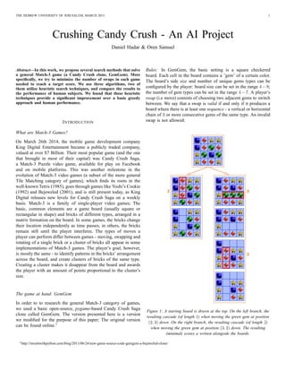
Figure 1: A starting board is drawn at the top. On the left branch, the
resulting cascade (of length 1) when moving the green gem at position
(2, 3) down. On the right branch, the resulting cascade (of length 2)
when moving the green gem at position (3, 2) down. The resulting
(minimal) scores a written alongside the boards.

2. THE HEBREW UNIVERSITY OF JERUSALEM, MARCH 2015 2
Once a valid swap is performed, the following process is initiated:
1) The gems in the created sequence(s) are cleared, rendering
their cells empty.
2) The gems which reside above the empty cells are pulled
down in a gravitational manner, filling the empty cells. The
fallen gems’ original cells become empty.
3) New gems appear (i.e “fall down”) in the now empty cells.
4) If the process creates new gem sequences, return to step 1.
Otherwise, wait for the player’s next swap.
This “chain reaction”, i.e a series of 1 or more such iterations,
is called a cascade. Once the the iteration process is finished, i.e
there are no remaining sequences on the board, we say that the
board is stable. See Figure 1 for an example.
If there are no valid swaps on the board, we say that we’ve reached
a game-over state.
Assumptions: Under the given rules, there are many ways one
could interpret some aspects of the game’s behavior. We tried to
be as straightforward as possible - the most neat interpretation
is also the best interpretation. Utilizing this approach, the game’s
behavior is defined in the following manner:
1) Clusters: If a swap creates a cluster (i.e an arbitrary
arrangement of consecutive same-colored gems), the board
is only cleared of gems that form parts of actual sequences.
Other gems in the cluster are kept on the board (see Figure
2). That is in contrast to some Match-3 variants where a
whole cluster is can be cleared from the board.
2) Randomization of appearing gems: The appearing gems
(that fill the empty spaces, created by cleared sequences) are
chosen uniformly at random. That is in disagreement with
the original implementation of GemGem, which prevented
from appearing gems to be identically-colored to their
neighbors on the board. When the game is configured such
that the number of gem types is small, this assumption
might cause very long cascades; however, violating this
assumption makes the game almost deterministic, which is
an even more undesirable trait.
3) Randomization of the initial board: Contrary to the
previous assumption, the initialization of the board is not
random. The board is initialized such that there are no
sequences - so no “free” points are given to the player,
and the playing field is leveled, so to speak, when starting
a game.
Scoring Method: A cascade awards the player p points, where p
is the number of gems cleared during the cascade. For example,
in Figure 1, the move presented in the right branch will yield a
score of at least 6. Similarly, the right branch in Figure 2 will
yield a score of at least 8.
We say at least because of assumption 2 mentioned before - ap-
pearing gems are randomized, therefore they can create sequences
with the gems already on the board - making the cascade longer
and clearing additional gems.
Figure 2: A starting board is drawn at the top. On the left branch, the
resulting sequence (of size 3) when moving the red gem at position
(3, 3) right. On the right branch, the resulting red cluster (of size 5) and
blue sequence (of size 3) when moving the blue gem at position (4, 3)
right. The resulting (minimal) scores are written below the boards.
Problem Definition
Once the rules of the game are well-defined, we can take on the
mission of defining the abstract problem that lies within the game.
There are many natural problems that arise from the given set of
rules. We’ve concluded that, from an AI point of view, there are
3 problems that would be interesting to tackle:
Given an s × s Match-3 board containing g types of gems, try to:
(P1) Minimize the number of swaps needed to reach a score
of at least c,
(P2) Maximize the score while performing at most k moves,
or
(P3) Perform as many moves as possible without reaching a
game-over state.
We’ve chosen to tackle P1; We will later describe possible
modifications to our approach that could tackle P2 and P3.
The problem is interesting because of the complexity of predicting
a large amount of possible future moves (similarly to chess-like
games) - thus AI tools are expected to improve the results when
compared to simpler algorithms and human subjects.
NP Completeness: Two papers, both published in March 2014,
took on proving that problems arising from Match-3 games are
NP-Complete.
The first paper, by Guala, Leucci and Natale2
, defines 5 such
2Gualà, L., Leucci, S., & Natale, E. (2014). Bejeweled, Candy Crush and other
Match-Three Games are (NP-) Hard. arXiv preprint arXiv:1403.5830. Full PDF
here: http://arxiv.org/abs/1403.5830

3. THE HEBREW UNIVERSITY OF JERUSALEM, MARCH 2015 3
problems (denoted Q1 through Q5). The first of which (Q1) is
formulated in the following manner: Is there a sequence of moves
that allows the player to pop a specific gem? The authors then go
on to prove that Q1 is NP-Complete. Then, Q2 through Q5 are
proven to be NP-Complete by reduction to Q1.
Q3 is of special interest to us, and is formulated as such: Can
the player get a score of at least c in less than k moves? This
problem is very similar to our problem (P1), and we can perform
a simple decision-to-search reduction from Q3 to P1: If we are to
minimize the number of swaps moves needed to achieve a score
c, we can check whether c is achievable within 1 move; if not,
check whether it’s achievable within 2 moves, and so on. The first
time we get a positive answer will give us the minimal number
of moves needed to reach score c. This, if so, implies that P1
is indeed NP-Complete. In a very similar approach, we can show
that P2 is NP-Complete. And, if we utilize Q5 from Guala’s paper,
we can show that P3 is NP-Complete as well. It is noteworthy that
the second paper, by Walsh3
, shows that Q3 is NP-Complete, too,
and does so by formulating a reduction to the 3-SAT problem.
Setting the Parameters: In our tests, the board size s is set to 6
and the number of gem types g is set to 4. The target score c
is set to 250. We took these decisions after running preliminary
tests over all of the possible combinations (s, g) ∈ {4, 5, 6, 7, 8}×
{4, 5, 6, 7}. Our analysis showed that when s/g ≤ 1, the proportion
of games reaching a premature game-over state (i.e ending before
the target score is reached) was ≥ 1
2 , and this proportion grows as
s/g decreases (see Figure 3). On the other hand, when s/g increases
and approaches 2, the game-over rate decreases dramatically, but
there are too many valid swaps on the board for our algorithms
to have a reasonable runtime. Therefore, we concluded that s = 6
and g = 4 (i.e s/g = 1.5) is a good compromise - there’s a
relatively small chance of reaching a dead-end (game-over state),
while the number of valid swaps is small enough that we can run
thousands of games in a reasonable amount of time.
Figure 3: Game-over rate as a function of s/g
3Walsh, T. (2014). Candy Crush is NP-hard. arXiv preprint arXiv:1403.1911.
Full PDF here: http://arxiv.org/abs/1403.1911
APPROACH AND METHODS
Why Search?
Generally speaking, the problem at hand requires us, given a game
board, to choose a minimal series of swaps which will beat a
certain score. The natural approach to this kind of problem, which
we indeed chose, is to use search techniques - where the state
space is the set of all possible boards, and the transitions are valid
swaps that transform one board to another. Another somewhat
natural approach is to use machine learning techniques - however,
it is not as suitable, because of the huge size of the problems state
space (“board space”). Roughly speaking, assuming each of the
s2
cells on the board can be filled by any of the g gem types,
the state space’s size is in the vicinity of gs2
. For our chosen
values (s = 6, g = 4) this results in a state space of size ∼ 272
.
This means that encountering he same board twice is unlikely,
and therefore learning the best swap to perform on a given board
is not a trivial task.
The Non-Determinism Question
Finding an optimal series of transitions through state space is a
relatively simple task when dealing with a deterministic world -
one where the result of a move can be predicted. In our problem,
however, this isn’t the case - since after every swap (and the
resulting cascade) random gems are dropped from the top of the
board, we’re dealing with a non-deterministic search problem.
Therefore, a simple application of a general search algorithm
cannot work in our case, and we have to resort to our own variants
of searching techniques.
Problem Representation
In order to represent the problem in search terms, we can
define the problem in the following manner: we are given a
graph G = V, E where V = {v : v is a board} and E =
{e = v1, v2 : v1, v2 ∈ V ; e is a swap that yields v2 from v1}.
The starting point of the graph is the start board. This is an
abstract definition that will help us think about the problem in
search terms; it does not, however, capture the non-determinism
described previously - more about this in the Methods section.
Methods
We implemented 3 algorithms and 5 heuristics (detailed below).
The first algorithm is a non-heuristic “stupid” baseline algorithm;
the other two decide which move to preform using a weighing
of the different heuristics. The average per-swap running times of
these algorithms are presented in Figure 5.
The Algorithms:
• Stupid Greedy Search (SGS): Given a board, the algorithm
finds all the valid swaps and computes their direct score,
i.e the number of gems about to be cleared solely from
the swap itself, without considering the (possibly) resulting
cascade. The chosen swap is the maximal swap with respect
to the direct score; if there are several maximal swaps, one of
them is chosen at random. This algorithm serves as a good
baseline, since as shown in the Results section, it gives a
good model for the behavior of human players.

4. THE HEBREW UNIVERSITY OF JERUSALEM, MARCH 2015 4
• Heuristic Greedy Search (HGS): Similarly to SGS, HGS
chooses the best swap that can be done in the current
board with respect to its immediate result (and hence the
title ’greedy’). Contrary to SGS, the score of each swap is
calculated including the predicted cascade, and is given based
on the different heuristics - different weights can be assigned
to each heuristic, and interesting weighted combinations
between them can be created.
• Limited Breadth First Search (L-BFS): Similarly to HGS,
L-BFS chooses the best move using simulation of cascades
and using heuristic scoring. Contrary to HGS, this algorithms
performs a look-ahead, or simulation, of several swaps, ef-
fectively performing a breadth-first search through the graph
of boards described earlier. The algorithm begins with the
start board as a root node. Then, all the possible swaps are
found, their resulting boards are calculated, and these boards
are added as nodes in the graph. The process is then applied
to all the new nodes, and the same process is performed
iteratively. The process stops when all nodes have reached
a state we call cutoff (and hence the ’limited’ part), which
means the at least one of two properties apply to the relevant
board:
– The board is in a game-over state.
– The board has reached a predefined uncertainty limit:
denote u = d
s2 where d is the total score of the swap
series leading up to the current board (i.e the number of
gems cleared in the current branch of the look-ahead)
and s is the board size. Then u is the uncertainty factor
of the board - it represents the percentage of the board
which is unknown to us. Therefore, if u passes a certain
(predetermined) uncertainty limit 0 ≤ U ≤ 1, we deem
he board “too uncertain” to continue looking ahead from.
For example, in Figure 1, the last board in the right
branch has an uncertainty factor of u = d
s2 = 6
42 =
0.375.
Finally, when all nodes are at a cutoff state, we say that they
are leaves of the search graph, and we chose the best move
by applying our heuristic to each leaf (and sometimes, to the
series of boards leading up to it).
The Heuristics:
• Score: The amount of cleared gems (cascade included).
When applied to the L-BFS algorithm, we use a variant of
this heuristic - the average score per swap in the swap series
leading up to a leaf node. This is done since we’re aiming
to minimize the number of swaps.
• Pairs: The number of pairs (adjacent gems of the same type)
that remain on the board after the cascade. In L-BFS, this is
applied to the last board in the simulation. The motivation
here is that a board with more pairs is better since it is more
promising in terms of future possible moves.
• Moves: The number of possible future moves in the resulting
board. In L-BFS, this is applied to the last board in the
simulation. The motivation is similar to the “Pairs” heuristic.
• Depth: The row where the swap was performed (1-based
counting from the top of the board). In L-BFS, we take
the average depth over the series of simulated swaps. The
motivation to use this value lies in the fact that deeper swaps
cause more gems to move - a deep vertical sequence, when
cleared, causes the entire column above it to “fall down”,
whereas a shallow sequence results only in the movement of
the appearing gems.
• Touching: The number of gems that will have new neighbors
after the cascade (i.e. the “frame” of the appearing gems), in
a 4-neighbors fashion. The idea is that a higher ’Touching’
value implies a higher chance of large cascades.
Figure 4: Starting with the board on the top, we swap the red gem at
(2, 4) with the green gem at (2, 3). The heuristic values for the
resulting (bottom) board will be: Score - 3; Depth - 4; Pairs - 4; Moves
- 1; and Touching - 7.
Figure 5: Average running time for a single swap choice
(logarithmically scaled), for each algorithm (for L-BFS - also with
different uncertainty limits).
Implementation Issues
• Simulation of Appearing Gems: In L-BFS, when predicting
future boards (derived from simulated swaps), we had to
decide how to approach the appearing gems. On the one hand,
we can simulate them using the same distribution function
used when actually generating the gems (see assumption 2)
and take them into account when looking for swaps in a

5. THE HEBREW UNIVERSITY OF JERUSALEM, MARCH 2015 5
future board. On the other hand, we can view the cleared
cells as empty, and opt to use only the gems that we know
for certain will exist in that board. In favor of the first
approach is the fact that it tries to mimic the real behavior
of the game, so it might give a better prediction of the gems
on the board after several swaps. However, a similar gem
distribution does not guarantee a similar gem arrangement -
and the arrangement, which is unpredictable, has a crucial
effect on all of the heuristic values. In favor of the second
one is the fact that every predicted swap will almost certainly
be a valid future swap - as opposed to the first approach,
where we might predict swaps (and cascades) on gems that
will never actually exist. We ruled in favor of the second
approach, as it avoids the exaggerated promotion of high-
scoring imaginary swaps that will not be valid in the future
boards. Preliminary tests supported our intuition and gave
worse results when simulating appearing gems; we saw that
oftentimes the algorithm chooses a swap based on false
predictions.
• Reevaluation Timing (Sequence vs. Single move): As
stated before, in each L-BFS step we predict paths from the
current board until we reach a cutoff. Once choosing the
best leaf node, we are faced with two options: either perform
the entire sequence of swaps leading up to the leaf, or only
perform the first one. One main advantage of the sequence
approach is running time - we only need to search through
the board space once every few swaps, whereas in the single
step approach we need to search after every swap. However,
the sequence approach might, in some cases, cause us to try
invalid swaps. We opted for the more deterministic single-
step approach.
• Calibration of the Uncertainty Limit U: Intuitively, U
should be well below 0.5 - for if we don’t know the contents
of more than half the board, our swap choices will surely
be poor. However, if it is set too low, L-BFS might be too
limited with respect to the length of the simulated swap
series. Running time also has a say in this - setting U
too high might make the swap series too long for L-BFS
to run in a reasonable time (see Figure 5). We found that
setting U around 0.2 gives a good balance of the different
considerations.
Test Plan
We carried out a 3-tiered testing scheme, where the first two
tiers were aimed at calibrating the algorithms for the third, final,
testing tier. Needless to say, many of the implementation issues
previously described were solved by these tests. We denote our
five heuristic by hs (Score), hp (Pairs), hn (Moves), hd (Depth),
and ht (Touching). We denote their corresponding weights by ws,
wp, wn, wd, and wt. The vector [ws, wp, wn, wd, wt] is a
weight vector. The following describes the games we ran to test
our algorithms; the results are show in the next section.
1) Preliminary Tests:
a) 100 SGS games.
b) 5 human subjects, 10 games each.
2) Basic Heuristics and Combinations:
a) 30 games of HGS, with every
[ws, wp, wn, wd, wt] ∈ {0, 1}
5
(i.e, every
possible linear combination of the vectors in the
canonical basis of R5
).
b) 30 games of L-BFS with the same weights.
3) Weight Calibration:
a) 30 games of HGS: all possible weight vectors
[ws, wp, wn, wd, wt] over all the weights between
0 and 2, in 0.2 intervals (e.g [0.2, 0.4, 1.8, 0.4, 0] )
b) 30 games of L-BFS, with the same weight combina-
tions.
RESULTS
First we show in Figure 6 the basic results (i.e, the average
number of swaps required to reach a score of 250, over 30
games) when running each individual heuristic by itself (e.g using
a weight vector [0, 1, 0, 0, 0]). The average results of SGS and
human subjects are shown for comparison.
We can easily notice that the Score heuristic is the most prominent,
and the Moves and Pairs heuristics are consistently ineffective.
The Depth and Touching heuristics are somewhere in between.
Note that the same heuristic in the two different algorithms gives
a similar outcome (with L-BFS winning by a small margin), except
in the Touching heuristic, which behaves very differently.
Figure 6: Average results for individual heuristics, with SGS and
human averages for comparison.
The above results give a general idea of the effectiveness of
each individual heuristic. The next step is to look at their basic
combinations - i.e the set of all “canonical” weight vectors -
{0, 1}
5
. The results for these tests are shown in Figure 7.
As we saw before, when including the Score heuristic (the top half
of the graph in Figure 7), we get generally better results. These

6. THE HEBREW UNIVERSITY OF JERUSALEM, MARCH 2015 6
Figure 7: Average results for basic heuristic combinations, with SGS
and human averages for comparison.
results also hinted us that the Moves heuristic might be ineffective,
and in fact worsens our results. This ineffectiveness can be seen
in the graph presented in Figure 8 - indeed, the Moves heuristic
does not help us, at all, to lower the swap count. Therefore, in
the weight calibration process, we decided to omit it in further
testing.
In the next and final step, we performed a weight calibration, in
order to find the best weight vector (with wn zeroed out). Figure
9 shows the top 10 heuristic combinations.
We now proceed to analyze the above results.
ANALYSIS
When looking at the top 10 heuristic combinations, we can first
see that L-BFS has a small advantage over HGS - 6 of the top
10 (and 4 of the top 5) combinations utilize L-BFS. Moreover,
the top 2 combinations are L-BFS. When looking at the numbers,
achieving a swap count of less than 16 means that these algorithms
averaged over 15.7 points per move. This is a very good result
- it means that, in average, these algorithms cleared 44% of the
board in every swap. For comparison, human subjects averaged
8.9 points per move (clearing only 24% of the board, on average),
∼ 43% less
Figure 8: The average swap count when using the Score heuristic with
each of the other four (left) and when using each of the four non-Score
heuristics individually (right).
Figure 9: The top 10 heuristics and their average swap count. SGS and
human results are too far out to show (at 25.2 and 28.8, respectively)
It is obvious that the hs value is the most important factor,
followed by the hd value. This makes sense - we’re aiming to
minimize the number of swaps to reach a certain score, therefore
we’re aiming to maximize the score of each swap. As any beginner
Candy Crush player could tell - nothing beats a high scoring move
with a long cascade. That being said, using hs alone comes in at
a close second, after a combination using hs, hp, hd and ht.
The prominence of hs is more apparent in L-BFS than in HGS -
since L-BFS foresees several steps into the future, and therefore
is able to chose the swap with the best score in its horizon. HGS,
on the other hand, gains a larger benefit from the help of other
predictions, such as the hp and ht values, since hs on its own is

7. THE HEBREW UNIVERSITY OF JERUSALEM, MARCH 2015 7
not a good enough predictor when looking only one step ahead.
If we take a step back and observe the graph in Figure 6, we see
an anomaly mentioned before, regarding the ht value - when used
by itself, it yields good results when using HGS, in contrast to
very bad results when used in L-BFS. It is the only heuristic value
which presents this pattern. Our explanation for this behavior is the
chaotic nature of the ht value, when looking more than one step
ahead. In HGS, the ht value is the deterministic number neighbors
that the appearing gems will have after the move is performed;
while in L-BFS, the ht value of a swap is associated with the last
board in the series of swaps, where the “frame” for the appearing
gems might be very different. This is in contrast, for example,
to the hp value, where most pairs that exist on the last board in
the swap series will probably remain there after performing the
swaps.
Revisiting Figure 8, we want to explain the anomaly of hn (Move
heuristic) being an ineffective heuristic. Prior to the actual tests,
hn seemed to us as an efficient heuristic since a board with more
valid swaps is a more “promising” board, in terms of the number
of choices we can make. But as in life itself, the paradox of choice
appears also in GemGem, and the results showed us that a board
with more moves isn’t, in fact, better. This has two reasons. First,
high-scoring moves result in boards with fewer gems, and boards
with fewer gems generally contain less valid swaps - so using
a high wn value actually causes the algorithms to chose lower-
scoring moves. Second, the amount of moves isn’t necessarily
in correlation with their quality; for example one could easily
imagine a board with 2 valid swaps, where one swap yields a
board with k > 1 3-point valid swaps, and the other swap yields
a board with one 15-point swap - choosing the first one isn’t better.
CONCLUSIONS
Observing the outcomes of out tests, we were glad to see that
a computer algorithm can be significantly better than humans in
Candy Crush - this shows that it is not only a game of luck,
but also of strategy and calculation. Given different prediction
abilities, and utilizing a variety of heuristic calculations, the
computer’s results can vary widely, sometimes for the better, and
sometimes for the worse. We saw that, unsurprisingly, when trying
to maximize the score of a swap, using a score-based heuristic
yields the best results. However, other heuristic values, associated
with the placement of a swap on the board and the characteristics
of the board resulting from the swap, can have a positive effect
on the result, especially when performing a one-step prediction.
As for further research, there’s a lot that is left to uncover. First,
regarding the problem settings - we chose a specific board size and
number of gem types; even though changing these values keeps
the main idea of the problem the same, it might be the case that
our algorithms and heuristics will produce very different results
when testing them with different settings. Our code easily supports
this kind of modification, and one could easily take it from here.
Second, regarding the problem definition - as shown before, there
are many problems that can be defined using the basic Match-3
rules. We chose to minimize the number of swaps to achieve a
certain score, and the dual problem of maximizing the score within
a limited number of swaps is probably similar, since solutions for
both these problems aim to maximize the score-per-swap ratio.
The third problem we described, however, is substantially different
- maximize the number of swaps without reaching game-over. In
this problem the score doesn’t really count, so the methods we
could use to tackle it might be different - for example, the Moves
heuristic might perform well in this case. It is also much more
interesting in boards with a high s/g factor, as we saw previously.
Third, even the simplest Candy Crush levels offer more complex
challenges than score maximization - non-rectangular boards,
popping specific gems, special combo-candies which can pop the
gems around them, and many others. Each of these challenges can
be a research subject in itself.