1. One dimensional Wave Equation
2 2
y 2 y
c
t2 x2
(Vibrations of a stretched string)
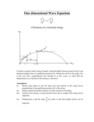
Y
T2
Q β
δs
P
α y
T1 δx
0 x x + δx A X
Consider a uniform elastic string of length l stretched tightly between points O and A and
displaced slightly from its equilibrium position OA. Taking the end O as the origin, OA
as the axis and a perpendicular line through O as the y-axis, we shall find the
displacement y as a function of the distance x and time t.
Assumptions
(i) Motion takes places in the XY plane and each particle of the string moves
perpendicular to the equilibrium position OA of the string.
(ii) String is perfectly flexible and does not offer resistance to bending.
(iii) Tension in the string is so large that the forces due to weight of the string can be
neglected.
y
(iv) Displacement y and the slope are small, so that their higher powers can be
x
neglected.

2. Let m be the mass per unit length of the string. Consider the motion of an element PQ of
length δs. Since the string does not offer resistance to bending(by assumption), the
tensions T1and T2 at P and Q respectively are tangential to the curve.
Since there is no motion in the horizontal direction, we have
T1cosα = T2cosβ = T(constant) …..(1)
Mass of element PQ is mδs.
By Newton’s second law of motion, the equation of motion in the vertical direction is
2
y
m s T2 sin T1 sin
x2
2
y T T
m s 2 sin sin ( from(1))
x cos cos
2
y T
2
(tan tan )
t m s
2
y T y y
2
t m x x x x x x
y y
2
y T x x x x x
2
t m x
2
y T 2y
, as x 0
t2 m x2
2 2
y y T
2
c 2 2 , where c 2
t x m
This is the partial differential equation giving the transverse vibrations of the string. It is
also called the one-dimensional wave equation.
Boundary conditions
For every value of t, y = 0 when x = 0
y = 0 when x = l
Initial conditions
If the string is made to vibrate by pulling it into a curve y=f(x) and then releasing it, the
initial conditions are
(i) y = f(x) when t = 0
y
(ii) 0 when t = 0
t

3. Solution of one-dimensional Wave Equation: -
The vibrations of the elastic string, such as a violin string, are governed by the one-
dimensional Wave equation
2 2
y 2 y T
2
c 2
, c2
t x m
----------------------------
------(1)
Let
y(x, t)=F(x)G(t)
-----------------------
--------(2)
be a solution of (1), where F(x) is only a function of x and G(t) is only a function of t only. On
differentiating equation (5), we obtain
2  2
y y
2
F G and FG
t x2
Where dot denotes the partial derivatives with respect to t and primes derivatives with respect to
x. By inserting this into differential equation (1), we have
..
F G c 2 F"G . Dividing c2 F"G we find

G F"
c 2G F
The left-hand side and Right-hand side of the above equation are function of t and x respectively
and both x & t are independent variables & hence both sides must be equal an they must be equal
to a some constant k.

G F"
k
c 2G F

4. This yields immediately two ordinary differential equations, namely
F”-kF=0
---------------------------------------------------------------
(6)
and
..
G kc 2 G 0 ---------------------------------------------------------------(7)
Satisfying the boundary conditions: -
We shall now determine solution F & G so that u=FG satisfies the boundary conditions.
u(0, t)=F(0).G(t)=0 ; u(l, t)=F(L)G(t)=0
Solving (6) If G=0 then u=0 which is of no interest and then
(a) F(0)=0 (b) F(L)=0
-------------------------------------------(8)
So, here three cases arise.
Case-I (k=0) then the general solution of (6) is F=ax+b. Now applying (8) we obtain a=b=0, and
hence F 0, which is of no interest because then u 0.
Case-II (k>0 and k= 2) then general solution of (6) is F=Ae x
+ Be- x
and again applying (8),
we get F 0 & hence u 0. So we discard the case k= 2.
Case-III (k<0 and k=-p2) Then the differential equation (6) takes the form
F”+p2F=0.

5. Its general solution is
F(x)=Acos px +B sin px
Applying (8), we obtain
F(0)=0=A(1) +B(0)
A=0.
and
F(L)=0 BsinpL=0.
We must take B 0 since otherwise F 0. Hence, sinpL=0 pL=n
n
p (n integer)
L
-----------------------------------------------(9)
We thus obtain infinitely many solutions F(x)=Fn(x) n=1,2,3--------
n x
Fn ( x ) B n sin
L
----------------------------------------------------------(10)
These solutions satisfy the equation (8).
Solving (7), the constant k is now restricted to the values k=-p2
2
n
k
L
..
2 n c
Inserting to the equation (7), we get G n Gt 0 where n ,
L
A general solution is G n t a n cos n t b n sin n t

6. And hence yn x, t Fn x .Gn t
n c n c n x
yn x , t an cos t bn sin t sin
l l l
---------(11)
Using principle of superposition the general solution is given by
y x, t yn x , t
n 1
n c n c n x
y x, t an cos t bn sin t sin
n 1 l l l -------------(12)
y
Now applying the initial conditions y = f(x) and 0 , when t = 0 , we have
t
n x
f ( x) an sin ............(13)
n 1 l
n c n x
0 bn sin .............(14)
n 1 l l
Since eqn.(13) represents Fourier series for f(x), we have
1
2 n x
an f ( x)sin dx .............(15)
l 0 l
From (14), bn = 0 for all n.
Hence (12) reduces to
n c n x
y x, t an cos t sin .................(16)
n 1 l l
Where an is given by (15)

7. Examples
1. A string is stretched and fastened to two points l apart. Motion is started by displacing the
x
string in the form y a sin from which it is released at time t=0. Show that the
l
displacement of any point at a distance x from one end at time t is given by
x ct
y ( x, t ) a sin cos
l l
2. The points of trisection of a string are pulled aside through the same distance on opposite
sides of the position of equilibrium and the string is released from rest. Derive an
expression for the displacement of the string at subsequent time and show that the mid-
point of the string always remains at rest.
9a 1 2m 2m ct 2m x
y ( x, t ) 2 2
sin cos sin , for n 2m
m 1m 3 l l
Ans.
l
y ,t 0, sin ce sin m 0
2
3. A tightly stretched string with fixed end points x=0 and x=l is initially at rest in its
equilibrium position. If it is set vibrating by giving to each of its points a velocity λx(1-x), find
the displacement of the string at any distance x from one end at any time t.
Ans.
8 l3 1 (2m 1) ct (2m 1) x
y ( x, t ) 4
sin sin , for n 2m 1
c 4 m 1 2m 1 l l
H int : bn 0 when n is even
8 l2
, when n is odd
n3 3
Re place n by 2m 1