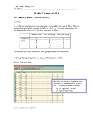
1. EDPR 7/8542, Spring 2005 1
Dr. Jade Xu
SPSS in Windows: ANOVA
Part I: One-way ANOVA (Between-Subjects):
Example:
In a verbal learning task, nonsense syllables are presented for later recall. Three different
groups of subjects see the nonsense syllables at a 1-, 5-, or 10-second presentation rate.
The data (number of errors) for the three groups are as follows:
1-second group 5-second group 10-second group
Number of 1 9 3
errors 4 8 5
5 7 7
6 10 7
4 6 8
The research question is whether the three groups have the same error rates.
Following the steps to perform one-way ANOVA analysis in SPSS:
Step 1: Enter your data.
Begin by entering your data in the same
manner as for an independent groups t-
test. You should have two columns:
1) the dependent variable
2) a grouping variable
Step 2: Define your variables.

2. EDPR 7/8542, Spring 2005 2
Dr. Jade Xu
Remember that to do this, you can simply double-click at the top of the variable’s
column, and the screen will change from “data view” to “variable view,” prompting you
to enter properties of the variable. For your dependent variable, giving the variable a
name and a label is sufficient. For your independent variable (the grouping variable), you
will also want to have value labels identifying what numbers correspond with which
groups. See the following figure for how to do this.
Start by clicking on the
cell for the “values” for
the variable you want.
The dialog box below
will appear.
Remember to click the
“Add” button each time you enter
a value label; otherwise,
the labels will not be added to
your variable’s properties.

3. EDPR 7/8542, Spring 2005 3
Dr. Jade Xu
Step 3: Select Oneway ANOVA from the command list in the menu as follows:
Note: There is more than one way to run ANOVA analysis in SPSS. For now, the
easiest way to do it is to go through the “compare means” option. However, since the
analysis of variance procedure is based on the general linear model, you could also use
the analyze/general linear model option to run the ANOVA. This command allows for
the analysis of much, much more sophisticated experimental designs than the one we
have here, but using it on these data would yield the same result as the One-way ANOVA
command.

4. EDPR 7/8542, Spring 2005 4
Dr. Jade Xu
Step 4: Run your analysis in SPSS.
Once you’ve selected the One-way ANOVA, you will get a dialog box like the one at the
top. Select your dependent and grouping variables (notice that unlike in the independent
samples t-test, you do not need to define your groups—SPSS assumes that you will
include all groups in the analysis.
While you’re here, you might as well
select the “options…” button, and check
that you would like descriptive and HOV
statistics. Another thing you might need
is the Post Hoc tests. You can also select
for SPSS to plot the means if you like.

5. EDPR 7/8542, Spring 2005 5
Dr. Jade Xu
Step 5: View and interpret your output.
Note that the descriptive statistics include
Confidence Intervals, your test of
homogeneity of variance is in a separate
table from your descriptive, and your
ANOVA partitions your sum of squares.
If you wish to do this with syntax commands, you can see what the syntax looks like by
selecting “paste” when you are in the One-way ANOVA dialog box.
Step 6: Post-hoc tests
Once you have determined that differences exist among the group means, post hoc
pairwise and multiple comparisons can determine which means differ. SPSS presents
several choices, but different post hoc tests vary in their level by which they control Type
I error. Furthermore, some tests are more appropriate than other based on the
organization of one's data. The following information focuses on choosing an
appropriate test by comparing the tests.

6. EDPR 7/8542, Spring 2005 6
Dr. Jade Xu
A summary leading up to using a Post Hoc (multiple comparisons):
Step 1. Test homogeneity of variance using the Levene statistic in SPSS.
a. If the test statistic's significance is greater than 0.05, one may assume equal
variances.
b. Otherwise, one may not assume equal variances.
Step 2. If you can assume equal variances, the F statistic is used to test the hypothesis. If
the test statistic's significance is below the desired alpha (typically, alpha = 0.05),
then at least one group is significantly different from another group.
Step 3. Once you have determined that differences exist among the means, post hoc
pairwise and multiple comparisons can be used to determine which means differ.
Pairwise multiple comparisons test the difference between each pair of means,
and yield a matrix where asterisks indicate significantly different group means at
an alpha level of 0.05.
Step 4. Choose an appropriate post hoc test:
a. Unequal Group Sizes: Whenever you violate the equal n assumption for groups,
select any of the following post hoc procedures in SPSS: LSD, Games-Howell,
Dunnett's T3, Scheffé, and Dunnett's C.
b. Unequal Variances: Whenever you violate the equal variance assumption for
groups (i.e., the homogeneity of variance assumption), check any of the following
post hoc procedures in SPSS: Tamhane’s T2, Games-Howell, Dunnett's T3, and
Dunnett's C.

7. EDPR 7/8542, Spring 2005 7
Dr. Jade Xu
c. Selecting from some of the more popular post hoc tests:
Fisher's LSD (Least Significant Different): This test is the most liberal of all
Post Hoc tests and its critical t for significance is not affected by the number
of groups. This test is appropriate when you have 3 means to compare. It
is not appropriate for additional means.
Bonferroni (AKA, Dunn’s Bonferroni): This test does not require the overall
ANOVA to be significant. It is appropriate when the number of
comparisons (c = number of comparisons = k(k-1))/2) exceeds the number
of degrees of freedom (df) between groups (df = k-1). This test is very
conservative and its power quickly declines as the c increases. A good rule of
thumb is that the number of comparisons (c) be no larger than the degrees of
freedom (df).
Newman-Keuls: If there is more than one true null hypothesis in a set of
means, this test will overestimate they familywise error rate. It is
appropriate to use this test when the number of comparisons exceeds the
number of degrees of freedom (df) between groups (df = k-1) and one does
not wish to be as conservative as the Bonferroni.
Tukey's HSD (Honestly Significant Difference): This test is perhaps the most
popular post hoc. It reduces Type I error at the expense of Power. It is
appropriate to use this test when one desires all the possible comparisons
between a large set of means (6 or more means).
Tukey's b (AKA, Tukey’s WSD (Wholly Significant Difference)): This test
strikes a balance between the Newman-Keuls and Tukey's more conservative
HSD regarding Type I error and Power. Tukey's b is appropriate to use
when one is making more than k-1 comparisons, yet fewer than (k(k-1))/2
comparisons, and needs more control of Type I error than Newman-
Kuels.
Scheffé: This test is the most conservative of all post hoc tests. Compared to
Tukey's HSD, Scheffé has less Power when making pairwise (simple)
comparisons, but more Power when making complex comparisons. It is
appropriate to use Scheffé's test only when making many post hoc
complex comparisons (e.g. more than k-1).
End note:
Try to understand every piece of information presented in the output. Button-clicks in
SPSS are not hard, but as an expert, you are expected to explain the tables and figures
using the knowledge you have learned in class.

8. EDPR 7/8542, Spring 2005 8
Dr. Jade Xu
Part II: Two-way ANOVA (Between-Subjects):
Example:
A researcher is interested in investigating the hypotheses that college achievement is
affected by (1) home-schooling vs. public schooling, (2) growing up in a dual-parent
family vs. a single-parent family, and (3) the interaction of schooling and family type.
She locates 5 people that match the requirements of each cell in the 2 × 2 (schooling ×
family type) factorial design, like this:
Schooling
Home Public
Family type Dual Parent
Single Parent
Again, we’ll do the 5 steps of hypothesis testing for each F-test. Because step 5 can be
addressed for all three hypotheses in one fell swoop using SPSS, that will come last.
Here are the first 4 steps for each hypothesis:
A. The main effect of schooling type
1. ;
2. F
3. N = 20; F(1,16)
4. ,
B. The main effect of family type
1. ;
2. F
3. N = 20; F(1,16)
4. ,
C. The interaction effect
1. ;
2. F
3. N = 20; F(1,16)
4. ;
Step 5, using SPSS

9. EDPR 7/8542, Spring 2005 9
Dr. Jade Xu
Following the steps to perform two-way ANOVA analysis in SPSS:
Step 1: Enter your data.
Because there are two factors, there are now two columns for "group": one for family
type (1: dual-parent; 2: single-parent) and one for schooling type (1: home; 2: public).
Achievement is placed in the third column. Note: if we had more than two factors, we
would have more than two group columns. See how that works? Also, if we had more
than 2 levels in a given factor, we would use 1, 2, 3 (etc.) to denote level.
Step 2. Choose Analyze -> General Linear Model -> Univariate...

10. EDPR 7/8542, Spring 2005 10
Dr. Jade Xu
Step 3. When you see a pop-up window like this one below, plop Fmly_type and
Schooling into the "Fixed Factors" window and Achieve into the "Dependent Variable"
window...
In this window, you might as well
select the “options…” button, and
check that you would like descriptive
and HOV statistics. Another thing you
might need is the Post Hoc tests. You
can also select for SPSS to plot the
means if you like.
...and click on "OK," yielding:
Tests of Between-Subjects Effects
Dependent Variable: Achieve
Type III Sum
Source of Squares df Mean Square F Sig.
Corrected Model 1.019(a) 3 .340 41.705 .000
Intercept 4.465 1 4.465 548.204 .000
Fmly_type .045 1 .045 5.540 .032
Schooling .465 1 .465 57.106 .000
Fmly_type * Schooling .509 1 .509 62.468 .000
Error .130 16 .008
Total 5.614 20
Corrected Total 1.149 19
a R Squared = .887 (Adjusted R Squared = .865)
I have highlighted the important parts of the summary table. As with the one-way
ANOVA, MS = SS/df and F = MSeffect / MSerror for each effect of interest. Also, values
add up to the numbers in the "Corrected Total" row.
An effect is significant if p< α or, equivalently, if Fobs / Fcrit. The beauty of SPSS is that
we don't have to look up a Fcrit if we know p. Because p< α for each of the three effects
(two main effects and one interaction), all three are statistically significant.
One way to plot the means (I used SPSS for this – the "Plots" option in the ANOVA
dialog window) is:

11. EDPR 7/8542, Spring 2005 11
Dr. Jade Xu
The two main effects and interaction effect are very clear in this plot. It would be very
good practice to conduct this factorial ANOVA by hand and see that the results match
what you get from SPSS.
Here is the hand calculatioin. First, degrees of freedom...
Note that these df match those in the ANOVA summary table.
Next, the means...

12. EDPR 7/8542, Spring 2005 12
Dr. Jade Xu
Then, sums of squares...
...and by subtraction for the remaining ones:
Note that these sums of squares match those in the ANOVA summary table. So the F-
values are:

13. EDPR 7/8542, Spring 2005 13
Dr. Jade Xu
Note that these F values are within rounding error of those in the ANOVA summary
table.
According to Table C.3 (because α =.05 ), the critical value for all three F-tests is 4.49.
All three Fs exceed this critical value, so we have evidence for a main effect of family
type, a main effect of schooling type, and the interaction of family type and schooling
type. This agrees with our intuition based on the mean plots.
In the current example, a good way to organize the data is :
Schooling
Home Public Mean(i)
Dual Parent 0.50 0.54
0.30 0.29
0.43 0.31
0.52 0.47
0.41 0.48
Mean(1j) 0.432 0.418 0.425
Single Parent 0.12 0.88
0.32 0.69
0.22 0.91
0.19 0.86
0.19 0.82
Mean(2j) 0.208 0.832 0.520
Mean(j) 0.320 0.625 0.4725
Note: Post-hoc tests
Once you have determined that differences exist among the group means, post hoc
multiple comparisons can determine which means differ.

14. EDPR 7/8542, Spring 2005 14
Dr. Jade Xu
Part III: One-way Repeated Measures ANOVA (Within-Subjects):
The Logic
Just as there is a repeated measures or dependent samples version of the Student t test,
there is a repeated measures version of ANOVA. Repeated measures ANOVA follows
the logic of univariate ANOVA to a large extent. As the same participants appear in all
conditions of the experiment, however, we are able to allocate more of the variance. In
univariate ANOVA we partition the variance into that caused by differences within
groups and that caused by differences between groups, and then compare their ratio. In
repeated measure ANOVA we can calculate the individual variability of participants as
the same people take part in each condition. Thus we can partition more of the error (or
within condition) variance. The variance caused by differences between individuals is
not helpful when deciding whether there is a difference between occasions. If we can
calculate it we can subtract it from the error variance and then compare the ratio of error
variance to that caused by changes in the independent variable between occasions. So
repeated measures allows us to compare the variance caused by the independent variable
to a more accurate error term which has had the variance caused by differences in
individuals removed from it. This increases the power of the analysis and means that
fewer participants are needed to have adequate power.
The Model
For the sake of simplicity, I will demonstrate the analysis by using the following three
participants that were measured in four occasions.
Participant Occasion 1 Occasion 2 Occasion 3 Occasion 4
1 7 7 5 5 ∑ = 24
2 6 6 5 3 ∑ = 20
3 5 4 4 3 ∑ = 16
∑ =18 ∑ = 17 ∑ = 14 ∑ = 11
SPSS Analysis
Step 1: Enter the data

15. EDPR 7/8542, Spring 2005 15
Dr. Jade Xu
When you enter the data remember that it consists of three participants measured on four
occasions and each row is for a separate participant. Thus, for this data you have three
rows and four variables, one for each occasion.
Step 2. To perform a repeated measures ANOVA you need to go through Analyze to
General Linear Model, which is where you found one of the ways to perform Univariate
ANOVA. This time, however, you click on Repeated Measures.
After this the following
dialogue box should appear.
The dialogue box refers to the occasions as a
within subjects factor and it automatically
labels it factor 1. You can if you want give
it a different name one which has meaning
for the particular data set you are looking at.
Although SPSS knows that there is a within
subjects factor, it does not know how many levels of it there are, in other words it does
not know how many occasions you tested you subjects. Here you need to type in 4 then
click on the Add button and then the Define button, which will let you tell SPSS which
occasions you want to compare. If you do this the following dialogue box will appear.

16. EDPR 7/8542, Spring 2005 16
Dr. Jade Xu
Next we need to put the variables into the within subjects box; as you can see we have
already put occasion 1 in slot (1) and occasion 2 in slot (2). We could also ask for some
descriptive statistics by going to Options and selecting Descriptives, once this is done
press OK and the following output should appear.
General Linear Model
Within-Subjects Factors
Measure: MEASURE_1
Dependent
FACTOR1 Variable
1 OCCAS1 This first box just tells
2 OCCAS2 us what the variables are
3 OCCAS3
4 OCCAS4

17. EDPR 7/8542, Spring 2005 17
Dr. Jade Xu
Descriptive Statistics
Mean Std. Deviation N
occasion 1 6.0000 1.0000 3 From the descriptives, it is
occasion 2 5.6667 1.5275 3 clear that the means get
occasion 3 4.6667 .5774 3 smaller over occasions. The
occasion 4 3.6667 1.1547 3 box below should be ignored.
Multivariate Testsb
Effect Value F Hypothesis df Error df Sig.
FACTOR1 Pillai's Trace .a . . . .
Wilks' Lambda .a . . . .
Hotelling's Trace .a . . . .
Roy's Largest Root .a . . . .
a. Cannot produce multivariate test statistics because of insufficient residual degrees of
freedom.
b.
Design: Intercept
Within Subjects Design: FACTOR1
b
Mauchly's Test of Sphericity
Measure: MEASURE_1
a
Epsilon
Approx. Greenhous
Within Subjects Effect Mauchly's W Chi-Square df Sig. e-Geisser Huynh-Feldt Lower-bound
FACTOR1 .000 . 5 . .667 . .333
Tests the null hypothesis that the error covariance matrix of the orthonormalized transformed dependent variables is
proportional to an identity matrix.
a. May be used to adjust the degrees of freedom for the averaged tests of significance. Corrected tests are displayed in the
Tests of Within-Subjects Effects table.
b.
Design: Intercept
Within Subjects Design: FACTOR1
This box gives a measure of sphericity. Sphericity is similar to the assumption of
homogeneity of variances in Univariate ANOVA. It is a measure of the
homogeneity of the variances of the differences between levels. That is in this case
that the variance of the difference between occasion 1 and 2 is similar to that
between 3 and 4 and so on. Another way to think of it is that it means that
participants are performing in similar ways across the occasions. If the Mauchly test
statistic is not significant then we use the sphericity assumed F value in the next box.
If it is significant then we should use the Greenhouse-Geisser corrected F value. In
this case there are insufficient participants to calculate Mauchly. Try adding one
more participant who scores four on every occasion and check the sphericity.

18. EDPR 7/8542, Spring 2005 18
Dr. Jade Xu
Tests of Within-Subjects Effects
Measure: MEASURE_1
Type III Sum
Source of Squares df Mean Square F Sig.
FACTOR1 Sphericity Assumed 10.000 3 3.333 10.000 .009
Greenhouse-Geisser 10.000 2.000 5.000 10.000 .028
Huynh-Feldt 10.000 . . . .
Lower-bound 10.000 1.000 10.000 10.000 .087
Error(FACTOR1) Sphericity Assumed 2.000 6 .333
Greenhouse-Geisser 2.000 4.000 .500
Huynh-Feldt 2.000 . .
Lower-bound 2.000 2.000 1.000
This is the most important box for repeated measures ANOVA. As you can see the F
value is 10.
Tests of Within-Subjects Contrasts
Measure: MEASURE_1
Type III Sum
Source FACTOR1 of Squares df Mean Square F Sig.
FACTOR1 Linear 9.600 1 9.600 48.000 .020
Quadratic .333 1 .333 1.000 .423
Cubic 6.667E-02 1 6.667E-02 .143 .742
Error(FACTOR1) Linear .400 2 .200
Quadratic .667 2 .333
Cubic .933 2 .467
The Within-Subjects contrast box test for significant trends. In this case there is a
significant linear trend, which means in this case there is a tendency for the data to fall on
a straight line. In other words the mean for occasion 1 is larger than occasion 2 which is
larger than occasion 3 which is larger than occasion 4. If we have a quadratic trend we
would have an inverted U or a U shaped pattern. It is important to remember that this
box is only of interest if the overall F value is significant and that it is a test of a trend not
a specific test of differences between occasions. For that we need to look at post hoc
tests.
Hand Calculation:
It would be very good practice to conduct this repeated-measures ANOVA by hand and
see that the results match what you get from SPSS. The only formula needed is the
formula for the sum of squares that we used for univariate ANOVA; ∑x2 - (∑x )2/n.

19. EDPR 7/8542, Spring 2005 19
Dr. Jade Xu
The first step is to calculate the total variability or the total sum of squares (SST). It will
not surprise you to learn that this is the same as you were doing a univariate ANOVA.
That is, (49+49+25+25+36+36+25+9+25+16+16+9) - (60)2/12 = 320 - 300 = 20.
We now calculate the variability due to occasions. This variability is calculated exactly
the same way as the within group variability is calculated for a univariate ANOVA. So
for this data the variability due to occasions is the sum of the variability within each
occasion.
The variability for occasion 1 is (49+36+25) - (18)2 /3; for occasion 2 it is (49+36+16) -
172/3. See if you can work out the sum for occasions 3 and 4. The answers should
come to occasion 3 = 0.66 and occasion 4 = 2.66 and added to occasion 1 and 2, we get a
sum of 10. Again this is no surprise as it should be the same for within group variability
for a univariate ANOVA. This time, however, this variability is very important as it is
not a measure of error but a measure of the effect of the independent variable, as the
participants have remained the same but the independent variable has altered with the
occasion.
We now need to calculate the variation caused by individual variability, that is the three
participants in this study differ in their overall measures here. This calculation is
something we have not met in univariate ANOVA but the principles remain the same.
Looking at the data you can see that overall participant 1 had the highest score of 24,
participant 2 had an overall score of 20 and participant 3 had an overall score of 16.
To calculate individual variability we still use the sum of squares formula ∑x2 - (∑x )2/n.
In this case we get (242+202+162) - (60)2/3 = (576+400+256)-3600/3 = 32.
Alarm bells may be ringing as you will see that we have more variability than the total.
However, we have not adjusted this figure for the number of occasions; to do that we
divide in this instance by 4 to get a figure of 8. So the variability that is caused by
differences in participants is 8.
Another way to calculate the individual variability is to divide the squared row totals by
the number of occasions and then subtract the correction factor. This would give us;
242/4+202/4+162/4 = 308, and then subtracting the correction factor gives us 308-300 = 8.
At this stage we have calculated all of the variabilities that we need to perform our
analysis; the variability due to occasions that is caused by the differences in the
independent variable across occasions is 10, the variability due to differences in
individuals is 8 and the residual variability is 2. The residual or error variability is the
total variability (20) minus the sum of the variability due to occasions and individuals
(18).
The next step is to calculate the degrees of freedom so that we can turn these variabilities
into variances or mean squares (MS). The total degrees of freedom is 12 -1 =11, as in
the univariate ANOVA. The degrees of freedom for individuals is the number of
participants minus 1, in this case 3 -1=2 and for occasions it is the number of occasions

20. EDPR 7/8542, Spring 2005 20
Dr. Jade Xu
minus 1, in this case 4-1=3. The residual degrees of freedom is the total minus the sum
of the degrees of freedom from individuals and occasions; 11-5=6.
The mean squares are then calculated by dividing the variability by the degrees of
freedom. The mean square for individuals is 8/2=4, for occasions 10/3= 3.33 and for the
residual 2/6=0.33.
To calculate the F statistic it is important to remember that we are not interested in the
individual variability of subjects. This is part of the error variance which we cannot
control for in a univariate ANOVA, but which we can measure in a repeated measures
design and then discard. What we are concerned with is whether our independent
variable which changes on different occasions has an effect on subject's performance.
The F ratio we are interested in is, therefore, MSoccasions / MSresidual; 3.33/0.33 which is 10.
If you were calculating statistics by hand you would now need to go to a table of values
for Fcrit to work out whether it is significant or not. We won't do that we will just
perform the same calculation by SPSS and check the significance there.
Notes:
1. The information presented in this handout is modified from the following websites:
For one-way between-subjects ANOVA
http://courses.washington.edu/stat217/218tutorial2.doc
For two-way between-subjects ANOVA
http://www.unc.edu/~preacher/30/anova_spss.pdf
For post-hoc tests:
http://staff.harrisonburg.k12.va.us/~gcorder/test_post_hocs.html
For repeated-measures ANOVA:
http://psynts.dur.ac.uk/notes/Year2/redesdat/RepeatedmeasuresANOVA.htm
2. Other useful web resources include:
http://employees.csbsju.edu/rwielk/psy347/spssinst.htm
http://www.colby.edu/psychology/SPSS/
http://www.oswego.edu/~psychol/spss/spsstoc.html
http://webpub.alleg.edu/dept/psych/SPSS/SPSS1wANOVA.html