The document describes using the homotopy perturbation method (HPM) to solve the temperature distribution in a radiating fin. The HPM is applied to the nonlinear differential equation that governs the temperature distribution. This results in a perturbation series solution for the dimensionless temperature. The HPM solution is compared to the Adomian decomposition method (ADM) solution. Results show that the HPM provides more accurate results and is easier to implement than the ADM for this problem of finding the temperature distribution in a radiating fin.

1. Hindawi Publishing Corporation
Mathematical Problems in Engineering
Volume 2009, Article ID 831362, 8 pages
doi:10.1155/2009/831362
Research Article
Solution of Temperature
Distribution in a Radiating Fin Using
Homotopy Perturbation Method
M. J. Hosseini, M. Gorji, and M. Ghanbarpour
Department of Mechanical Engineering, Noshirvani University of Technology, P.O. Box 484, Babol, Iran
Correspondence should be addressed to M. Gorji, gorji@nit.ac.ir
Received 27 November 2008; Accepted 22 January 2009
Recommended by Saad A. Ragab
Radiating extended surfaces are widely used to enhance heat transfer between primary surface
and the environment. The present paper applies the homotopy perturbation to obtain analytic
approximation of distribution of temperature in heat fin radiating, which is compared with the
results obtained by Adomian decomposition method ADM . Comparison of the results obtained
by the method reveals that homotopy perturbation method HPM is more effective and easy to
use.
Copyright q 2009 M. J. Hosseini et al. This is an open access article distributed under the Creative
Commons Attribution License, which permits unrestricted use, distribution, and reproduction in
any medium, provided the original work is properly cited.
1. Introduction
Most scientific problems and phenomena such as heat transfer occur nonlinearly. Except a
limited number of these problems, it is difficult to find the exact analytical solutions for them.
Therefore, approximate analytical solutions are searched and were introduced 1–5 , among
which homotopy perturbation method HPM 6–12 and Adomain decomposition method
ADM 13, 14 are the most effective and convenient ones for both weakly and strongly
nonlinear equations.
The analysis of space radiators, frequently provided in published literature, for
example, 15–22 , is based upon the assumption that the thermal conductivity of the fin
material is constant. However, since the temperature difference of the fin base and its tip
is high in the actual situation, the variation of the conductivity of the fin material should be
taken into consideration and includes the effects of the variation of the thermal conductivity
of the fin material. The present analysis considers the radiator configuration shown in
Figure 1. In the design, parallel pipes are joined by webs, which act as radiator fins. Heat
flows by conduction from the pipes down the fin and radiates from both surfaces.

2. 2 Mathematical Problems in Engineering
2w
x
W b
Figure 1: Schematic of a heat fin radiating element.
Here, the fin problem is solved to obtain the distribution of temperature of the fin
by homotopy perturbation method and compared with the result obtained by the Adomian
decomposition method, which is used for solving various nonlinear fin problems 23–25 .
2. The Fin Problem
A typical heat pipe space radiator is shown in Figure 1. Both surfaces of the fin are radiating
to the vacuum of outer space at a very low temperature, which is assumed equal to zero
absolute. The fin is diffuse-grey with emissivity ε, and has temperature-dependent thermal
conductivity k, which depends on temperature linearly. The base temperature Tb of the fin
and tube surfaces temperature is constant; the radiative exchange between the fin and heat
pipe is neglected. Since the fin is assumed to be thin, the temperature distribution within the
fin is assumed to be one-dimensional. The energy balance equation for a differential element
of the fin is given as 26 :
d dT
2w k T − 2εσT 4 0, 2.1
dx dx
where k T and σ are the thermal conductivity and the Stefan-Boltzmann constant,
respectively. The thermal conductivity of the fin material is assumed to be a linear function
of temperature according to
K T Kb 1 λ T − Tb , 2.2
where kb is the thermal conductivity at the base temperature of the fin and λ is the slope of
the thermal conductivity temperature curve.
Employing the following dimensionless parameters:
3
T εσb2 Tb x
θ , ψ , ξ , β λTb , 2.3
Tb kw b
the formulation of the fin problem reduces to
2
d2 θ dθ d2 θ
β βθ − ψθ4 0, 2.4a
dξ2 dξ dξ2

3. Mathematical Problems in Engineering 3
with boundary conditions
dθ
0 at ξ 0, 2.4b
dξ
θ 1 at ξ 1. 2.4c
3. Basic Idea of Homotopy Perturbation Method
In this study, we apply the homotopy perturbation method to the discussed problems. To
illustrate the basic ideas of the method, we consider the following nonlinear differential
equation,
A θ −f r 0, 3.1
where A θ is defined as follows:
A θ L θ N θ , 3.2
where L stands for the linear and N for the nonlinear part. Homotopy perturbation structure
is shown as the following equation:
H θ, P 1 − p L θ − L θ0 p A θ −f r 0 3.3
Obviously, using 3.3 we have
H θ, 0 L θ − L θ0 0,
3.4
H θ, 1 A θ −f r 0,
where p ∈ 0, 1 is an embedding parameter and θ0 is the first approximation that satisfies the
boundary condition. We Consider θ and as
M
θ pi θi θ0 pθ1 p2 θ2 p3 θ3 p4 θ4 ··· . 3.5
i 0
4. The Fin Temperature Distribution
Following homotopy-perturbation method to 2.4a , 2.4b , and 2.4c , linear and non-linear
parts are defined as
d2 θ
L θ ,
dξ2
2 4.1
dθ d2 θ
N θ β βθ 2 − ψθ4 ,
dξ dξ
with the boundary condition given in 2.4b , θ 0 is any arbitrary constant, C.

4. 4 Mathematical Problems in Engineering
Then we have
dθ
0 at ξ 0, θ C at ξ 0. 4.2
dξ
Substituting 3.5 in to 4.1 and then into 3.3 and rearranging based on power of p-terms,
we have the following
p0
∂2
θ0 ξ 0, 4.3a
∂ξ2
dθ0
0 at ξ 0, θ0 C at ξ 0; 4.3b
dξ
p1
2
∂2 ∂2 ∂
θ1 ξ βθ0 ξ θ0 ξ β θ0 ξ − ψθ0 ξ
4
0, 4.4a
∂ξ2 ∂ξ2 ∂ξ
dθ1
0 at ξ 0, θ1 0 at ξ 0; 4.4b
dξ
p2
∂2 ∂2 ∂2
θ2 ξ βθ0 ξ θ1 ξ βθ1 ξ θ0 ξ
∂ξ2 ∂ξ2 ∂ξ2
4.5a
∂ ∂
2β θ0 ξ θ1 ξ − 3
4ψθ0 ξ θ1 ξ 0,
∂ξ ∂ξ
dθ2
0 at ξ 0, θ2 0 at ξ 0; 4.5b
dξ
p3
2
∂2 ∂2 ∂2 ∂
θ3 ξ βθ2 ξ θ0 ξ βθ0 ξ θ2 ξ β θ1 ξ
∂ξ2 ∂ξ2 ∂ξ2 ∂ξ
∂2 ∂ ∂ 4.6a
βθ1 ξ θ1 ξ 2β θ0 ξ θ2 ξ − 4ψθ0 ξ θ2 ξ
3
∂ξ2 ∂ξ ∂ξ
− 6ψθ0 ξ θ1 ξ
2 2
0,
dθ3
0 at ξ 0, θ3 0 at ξ 0; 4.6b
dξ

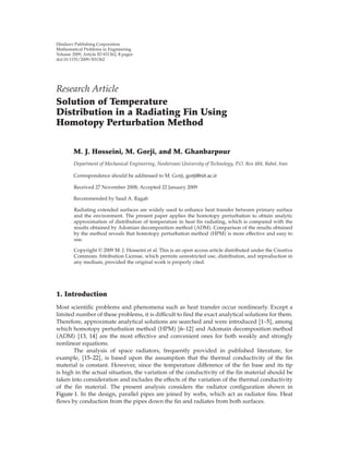
5. Mathematical Problems in Engineering 5
1
ψ 1
0.8
Dimensionless temperatrure, θ
0.6 ψ 10
0.4
ψ 100
0.2
0
0 0.2 0.4 0.6 0.8 1
Dimensionless coordinate, ξ
HPM
ADM
Figure 2: Comparison of the HPM and ADM for β 1.0 and M 14.
p4
∂2 ∂2 ∂2
θ4 ξ βθ3 ξ θ0 ξ βθ0 ξ θ3 ξ − 4ψθ0 ξ θ3 ξ
3
∂ξ2 ∂ξ2 ∂ξ2
∂2 ∂ ∂
βθ2 ξ θ1 ξ 2β θ0 ξ θ3 ξ − 12ψθ0 ξ θ2 ξ θ1 ξ
2
4.7a
∂ξ2 ∂ξ ∂ξ
∂2 ∂ ∂2
β θ1 ξ θ2 ξ βθ1 ξ θ2 ξ − 4ψθ0 ξ θ1 ξ
3
0,
∂ξ2 ∂ξ ∂ξ2
dθ4
0 at ξ 0, θ4 0 at ξ 0; 4.7b
dξ
and so forth.
By increasing the number of the terms in the solution, higher accuracy will be obtained.
Since the remaining terms are too long to be mentioned in here, the results are shown in tables.
Solving 4.3a , 4.4a , 4.5a , 4.6a , and 4.7a results in θ ξ . When p → 1, we have
1 1 2 7 4 1 5 2 13 3 10 6
θ ξ C ψC4 ξ2 ψ C ξ − βC ψξ ψ C ξ
2 6 2 180
11 2 8 4 1 2 6 2 23 4 13 8 19 3 11 6
− ψ C βξ β C ψξ ψ C ξ − ψ C βξ 4.8
24 2 720 60
7 2 9 2 4 1 3 7 2
β C ψ ξ − β C ψξ · · · .
8 2

6. 6 Mathematical Problems in Engineering
Table 1: The dimensionless tip temperature for ψ 1.
Number of the terms M 5 M 7 M 10 M 14
in the solution M
Method HPM ADM HPM ADM HPM ADM HPM ADM
β 0.6 0.827821 0.819185 0.826552 0.825079 0.8267319 0.825063 0.82675 0.825052
β 0.4 0.813389 0.814489 0.813351 0.813279 0.8133683 0.810866 0.813369 0.813236
β 0.2 0.797708 0.80021 0.797712 0.799025 0.7977122 0.797812 0.797712 0.797809
β 0 0.779177 0.777778 0.779147 0.777765 0.7791452 0.776554 0.779145 0.775333
β −0.2 0.757702 0.752987 0.75698 0.752967 0.7568182 0.754144 0.756802 0.754132
β −0.4 0.819743 0.814465 0.816013 0.813252 0.8132926 0.810831 0.812155 0.813201
β −0.6 0.710294 0.715063 0.703219 0.700812 0.6988481 0.696134 0.696764 0.694918
Table 2: The dimensionless tip temperature for ψ 1000.
Number of the terms M 5 M 7 M 10 M 14
in the solution M
Method HPM ADM HPM ADM HPM ADM HPM ADM
β 0.6 0.139382 0.144312 0.135502 0.137711 0.1330265 0.134125 0.132616 0.132718
β 0.4 0.138351 0.143412 0.134243 0.136526 0.1315594 0.132756 0.130091 0.131026
β 0.2 0.137341 0.142026 0.133009 0.134937 0.1301168 0.131213 0.129486 0.129613
β 0 0.136349 0.141055 0.131797 0.133785 0.1286995 0.129663 0.127504 0.127327
β −0.2 0.135376 0.140165 0.13061 0.132654 0.127308 0.128143 0.125348 0.125431
β −0.4 0.134422 0.139565 0.129445 0.131856 0.1259426 0.127342 0.124118 0.124432
β −0.6 0.133485 0.138374 0.128303 0.130525 0.1246034 0.125336 0.122715 0.122936
5. Results
The coefficient C representing the temperature at the fin tip can be evaluated from the
boundary condition given in 2.4c using the numerical method.
Tables 1 and 2 show the dimensionless tip temperature, that is, coefficient C, for
different thermal conductivity parameters, β. The tables state that the convergence of
the solution for the higher thermo-geometric fin parameter, ψ, is faster than the solution
with lower fin parameter. It is clear from the tables that the solution is convergent. In
order to investigate the accuracy of the homotopy solution, the problem is compared with
decomposition solution 26 , also the corresponding results are presented in Figure 2. It
should be mentioned that the homotopy results in the tables are arranged for first 5, 7, 10,
14 terms of the solution M . It is seen that the results by homotopy perturbation method,
and adomian decomposition method are in good agreement. The results of the comparison
show that the difference is 3.1% in the case of the strongest nonlinearity, that is, β 1.0 and
ψ 100.
6. Conclusions
In this work, homotopy perturbation method has been successfully applied to a typical
heat pipe space radiator. The solution shows that the results of the present method are in
excellent agreement with those of ADM and the obtained solutions are shown in the figure

7. Mathematical Problems in Engineering 7
and tables. Some of the advantage of HPM are that reduces the volume of calculations with
the fewest number of iterations, it can converge to correct results. The proposed method is
very simple and straightforward. In our work, we use the Maple Package to calculate the
functions obtained from the homotopy perturbation method.
References
1 E. M. Abulwafa, M. A. Abdou, and A. A. Mahmoud, “The solution of nonlinear coagulation problem
with mass loss,” Chaos, Solitons & Fractals, vol. 29, no. 2, pp. 313–330, 2006.
2 A. Aziz and T. Y. Na, Perturbation Methods in Heat Transfer, Series in Computational Methods in
Mechanics and Thermal Sciences, Hemisphere, Washington, DC, USA, 1984.
3 J.-H. He, “Some asymptotic methods for strongly nonlinear equations,” International Journal of Modern
Physics B, vol. 20, no. 10, pp. 1141–1199, 2006.
4 M. M. Rahman and T. Siikonen, “An improved simple method on a collocated grid,” Numerical Heat
Transfer Part B, vol. 38, no. 2, pp. 177–201, 2000.
5 A. V. Kuznetsov and K. Vafai, “Comparison between the two- and three-phase models for analysis
of porosity formation in aluminum-rich castings,” Numerical Heat Transfer Part A, vol. 29, no. 8, pp.
859–867, 1996.
6 J.-H. He, “Application of homotopy perturbation method to nonlinear wave equations,” Chaos,
Solitons & Fractals, vol. 26, no. 3, pp. 695–700, 2005.
7 J.-H. He, “Homotopy perturbation method for bifurcation of nonlinear problems,” International
Journal of Nonlinear Sciences and Numerical Simulation, vol. 6, no. 2, pp. 207–208, 2005.
8 J.-H. He, “Homotopy perturbation technique,” Computer Methods in Applied Mechanics and Engineering,
vol. 178, no. 3-4, pp. 257–262, 1999.
9 J.-H. He, “Variational iteration method for autonomous ordinary differential systems,” Applied
Mathematics and Computation, vol. 114, no. 2-3, pp. 115–123, 2000.
10 J.-H. He, “A coupling method of a homotopy technique and a perturbation technique for non-linear
problems,” International Journal of Non-Linear Mechanics, vol. 35, no. 1, pp. 37–43, 2000.
11 J.-H. He, “Homotopy perturbation method: a new nonlinear analytical technique,” Applied
Mathematics and Computation, vol. 135, no. 1, pp. 73–79, 2003.
12 J.-H. He, “The homotopy perturbation method for nonlinear oscillators with discontinuities,” Applied
Mathematics and Computation, vol. 151, no. 1, pp. 287–292, 2004.
13 G. Adomian, “A review of the decomposition method in applied mathematics,” Journal of
Mathematical Analysis and Applications, vol. 135, no. 2, pp. 501–544, 1988.
14 G. Adomian, Solving Frontier Problems of Physics: The Decomposition Method, vol. 60 of Fundamental
Theories of Physics, Kluwer Academic Publishers, Dordrecht, The Netherlands, 1994.
15 J. G. Bartas and W. H. Sellers, “Radiation fin effectiveness,” Journal of Heat Transfer, vol. 82C, pp. 73–75,
1960.
16 J. E. Wilkins Jr., “Minimizing the mass of thin radiating fins,” Journal of Aerospace Science, vol. 27, pp.
145–146, 1960.
17 B. V. Karlekar and B. T. Chao, “Mass minimization of radiating trapezoidal fins with negligible base
cylinder interaction,” International Journal of Heat and Mass Transfer, vol. 6, no. 1, pp. 33–48, 1963.
18 R. D. Cockfield, “Structural optimization of a space radiator,” Journal of Spacecraft Rockets, vol. 5, no.
10, pp. 1240–1241, 1968.
19 H. Keil, “Optimization of a central-fin space radiator,” Journal of Spacecraft Rockets, vol. 5, no. 4, pp.
463–465, 1968.
20 B. T. F. Chung and B. X. Zhang, “Optimization of radiating fin array including mutual irradiations
between radiator elements,” Journal of Heat Transfer, vol. 113, no. 4, pp. 814–822, 1991.
21 C. K. Krishnaprakas and K. B. Narayana, “Heat transfer analysis of mutually irradiating fins,”
International Journal of Heat and Mass Transfer, vol. 46, no. 5, pp. 761–769, 2003.
22 R. J. Naumann, “Optimizing the design of space radiators,” International Journal of Thermophysics, vol.
25, no. 6, pp. 1929–1941, 2004.
23 C. H. Chiu and C. K. Chen, “A decomposition method for solving the convective longitudinal fins
with variable thermal conductivity,” International Journal of Heat and Mass Transfer, vol. 45, no. 10, pp.
2067–2075, 2002.
24 C. H. Chiu and C. K. Chen, “Application of Adomian’s decomposition procedure to the analysis of
convective-radiative fins,” Journal of Heat Transfer, vol. 125, no. 2, pp. 312–316, 2003.

8. 8 Mathematical Problems in Engineering
25 D. Lesnic and P. J. Heggs, “A decomposition method for power-law fin-type problems,” International
Communications in Heat and Mass Transfer, vol. 31, no. 5, pp. 673–682, 2004.
26 C. Arslanturk, “Optimum design of space radiators with temperature-dependent thermal conductiv-
ity,” Applied Thermal Engineering, vol. 26, no. 11-12, pp. 1149–1157, 2006.

9. Journal of Applied Mathematics and Decision Sciences
Special Issue on
Decision Support for Intermodal Transport
Call for Papers
Intermodal transport refers to the movement of goods in Before submission authors should carefully read over the
a single loading unit which uses successive various modes journal’s Author Guidelines, which are located at http://www
of transport (road, rail, water) without handling the goods .hindawi.com/journals/jamds/guidelines.html. Prospective
during mode transfers. Intermodal transport has become authors should submit an electronic copy of their complete
an important policy issue, mainly because it is considered manuscript through the journal Manuscript Tracking Sys-
to be one of the means to lower the congestion caused by tem at http://mts.hindawi.com/, according to the following
single-mode road transport and to be more environmentally timetable:
friendly than the single-mode road transport. Both consider-
ations have been followed by an increase in attention toward Manuscript Due June 1, 2009
intermodal freight transportation research.
Various intermodal freight transport decision problems First Round of Reviews September 1, 2009
are in demand of mathematical models of supporting them. Publication Date December 1, 2009
As the intermodal transport system is more complex than a
single-mode system, this fact offers interesting and challeng-
ing opportunities to modelers in applied mathematics. This Lead Guest Editor
special issue aims to fill in some gaps in the research agenda Gerrit K. Janssens, Transportation Research Institute
of decision-making in intermodal transport. (IMOB), Hasselt University, Agoralaan, Building D, 3590
The mathematical models may be of the optimization type Diepenbeek (Hasselt), Belgium; Gerrit.Janssens@uhasselt.be
or of the evaluation type to gain an insight in intermodal
operations. The mathematical models aim to support deci-
sions on the strategic, tactical, and operational levels. The Guest Editor
decision-makers belong to the various players in the inter- Cathy Macharis, Department of Mathematics, Operational
modal transport world, namely, drayage operators, terminal Research, Statistics and Information for Systems (MOSI),
operators, network operators, or intermodal operators. Transport and Logistics Research Group, Management
Topics of relevance to this type of decision-making both in School, Vrije Universiteit Brussel, Pleinlaan 2, 1050 Brussel,
time horizon as in terms of operators are: Belgium; Cathy.Macharis@vub.ac.be
• Intermodal terminal design
• Infrastructure network configuration
• Location of terminals
• Cooperation between drayage companies
• Allocation of shippers/receivers to a terminal
• Pricing strategies
• Capacity levels of equipment and labour
• Operational routines and lay-out structure
• Redistribution of load units, railcars, barges, and so
forth
• Scheduling of trips or jobs
• Allocation of capacity to jobs
• Loading orders
• Selection of routing and service
Hindawi Publishing Corporation
http://www.hindawi.com

10. Fixed Point Theory and Applications
Special Issue on
Impact of Kirk’s Results in the Development of
Fixed Point Theory
Call for Papers
Kirk’s fixed point theorem published in 1965 had a profound Guest Editor
impact in the development of the fixed point theory over the
Tomas Domínguez-Benavides, Departamento de Análisis
last 40 years. Through the concept of generalized distance,
Matemático, Universidad de Sevilla, 41080 Sevilla, Spain;
Tarski’s classical fixed point theorem may be seen as a variant
tomasd@us.es
of Kirk’s fixed point theorem in discrete sets. This shows
among other things the power of this theorem.
This special issue will focus on any type of applications of
Kirk’s fixed point theorem. It includes:
• Nonexpansive mappings in Banach and metric spaces
• Multivalued mappings in Banach and metric spaces
• Monotone mappings in ordered sets
• Multivalued mappings in ordered sets
• Applications to nonmetric spaces like modular func-
tion spaces
• Applications to logic programming and directed gra-
phs
Before submission authors should carefully read over the
journal’s Author Guidelines, which are located at http://www
.hindawi.com/journals/fpta/guidelines.html. Articles publis-
hed in this Special Issue shall be subject to a reduced
Article Processing Charge of C200 per article. Prospective
authors should submit an electronic copy of their complete
manuscript through the journal Manuscript Tracking Sys-
tem at http://mts.hindawi.com/ according to the following
timetable:
Manuscript Due October 1, 2009
First Round of Reviews January 1, 2010
Publication Date April 1, 2010
Lead Guest Editor
M. A. Khamsi, Department of Mathematical Science,
University of Texas at El Paso, El Paso, TX 79968, USA;
mohamed@utep.edu
Hindawi Publishing Corporation
http://www.hindawi.com

11. International Journal of Mathematics and Mathematical Sciences
Special Issue on
Selected Papers from ICMS’10
Call for Papers
The First International Conference on Mathematics and Ayman Badawi, American University of Sharjah, P.O. Box
Statistics (ICMS’10), which will be held in Sharjah, UAE 26666, Sharjah, UAE; abadawi@aus.edu
(March 18–21, 2010) aims at bringing together researchers
Carl Cowen, Mathematical Sciences Building, Purdue
and scientists working in the fields of pure and applied
University, 150 N. University Street West, Lafayette, IN
mathematics, mathematics education, and statistics. The
47907, USA; ccowen@iupui.edu
proposed technical program of the conference will include
paper presentations and keynote lectures in algebra, analysis, Hana Sulieman, American University of Sharjah, P.O. Box
applied mathematics, applied statistics, differential equa- 26666, Sharjah, UAE; hsulieman@aus.edu
tions, discrete mathematics, financial mathematics, mathe-
matics education, number theory, numerical analysis, prob-
ability theory, statistics, stochastic differential equations,
topology, and geometry. Organizing this conference will help
build bridges between institutions and encourage interaction
among researchers from different disciplines from the region
and worldwide.
Authors will be required to rewrite their conference papers
as full-length manuscripts that extend substantially from
their conference submission. All papers will be rigorously
reviewed, and three review reports for each paper will be
solicited.
Before submission authors should carefully read over the
journal’s Author Guidelines, which are located at http://www
.hindawi.com/journals/ijmms/guidelines.html. Prospective
authors should submit an electronic copy of their complete
manuscript through the journal Manuscript Tracking Sys-
tem at http://mts.hindawi.com/ according to the following
timetable:
Manuscript Due May 1, 2010
First Round of Reviews August 1, 2010
Publication Date November 1, 2010
Lead Guest Editor
Mahmoud Anabtawi, American University of Sharjah,
P.O. Box 26666, Sharjah, UAE; manabtawi@aus.edu
Guest Editors
Zayid Abdulhadi, American University of Sharjah, P.O.
Box 26666, Sharjah, UAE; zahadi@aus.edu
Hindawi Publishing Corporation
http://www.hindawi.com