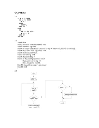
21221

CHAPTER 2
www.inKFUPM.com
2.1
IF x < 10 THEN
IF x < 5 THEN
x = 5
ELSE
PRINT x
END IF
ELSE
DO
IF x < 50 EXIT
x = x - 5
END DO
END IF

2.2
Step 1: Start
Step 2: Initialize sum and count to zero
Step 3: Examine top card.
Step 4: If it says “end of data” proceed to step 9; otherwise, proceed to next step.
Step 5: Add value from top card to sum.
Step 6: Increase count by 1.
Step 7: Discard top card
Step 8: Return to Step 3.
Step 9: Is the count greater than zero?
If yes, proceed to step 10.
If no, proceed to step 11.
Step 10: Calculate average = sum/count
Step 11: End

2.3
start

sum = 0
count = 0

T
count > 0
INPUT
value
F
average = sum/count
value = T
“end of data”

F end
sum = sum + value
count = count + 1

2.4
Students could implement the subprogram in any number of languages. The following
Fortran 90 program is one example. It should be noted that the availability of complex
variables in Fortran 90, would allow this subroutine to be made even more concise.
However, we did not exploit this feature, in order to make the code more compatible with
Visual BASIC, MATLAB, etc.
PROGRAM Rootfind
IMPLICIT NONE
INTEGER::ier
REAL::a, b, c, r1, i1, r2, i2
DATA a,b,c/1.,5.,2./
CALL Roots(a, b, c, ier, r1, i1, r2, i2)
IF (ier .EQ. 0) THEN
PRINT *, r1,i1," i"
PRINT *, r2,i2," i"
ELSE
PRINT *, "No roots"
END IF
END

SUBROUTINE Roots(a, b, c, ier, r1, i1, r2, i2)
IMPLICIT NONE
INTEGER::ier
REAL::a, b, c, d, r1, i1, r2, i2
r1=0.
r2=0.
i1=0.
i2=0.
IF (a .EQ. 0.) THEN
IF (b <> 0) THEN
r1 = -c/b
ELSE
ier = 1
END IF
ELSE
d = b**2 - 4.*a*c
IF (d >= 0) THEN
r1 = (-b + SQRT(d))/(2*a)
r2 = (-b - SQRT(d))/(2*a)
ELSE
r1 = -b/(2*a)
r2 = r1
i1 = SQRT(ABS(d))/(2*a)
i2 = -i1
END IF
END IF
END

The answers for the 3 test cases are: (a) −0.438, -4.56; (b) 0.5; (c) −1.25 + 2.33i; −1.25 −
2.33i.

Several features of this subroutine bear mention:
• The subroutine does not involve input or output. Rather, information is passed in and out
via the arguments. This is often the preferred style, because the I/O is left to the
discretion of the programmer within the calling program.
• Note that an error code is passed (IER = 1) for the case where no roots are possible.

2.5 The development of the algorithm hinges on recognizing that the series approximation of the
sine can be represented concisely by the summation,

n 2i −1
x
∑ (2i − 1)!
i =1

where i = the order of the approximation. The following algorithm implements this
summation:

Step 1: Start
Step 2: Input value to be evaluated x and maximum order n
Step 3: Set order (i) equal to one
Step 4: Set accumulator for approximation (approx) to zero
Step 5: Set accumulator for factorial product (fact) equal to one
Step 6: Calculate true value of sin(x)
Step 7: If order is greater than n then proceed to step 13
Otherwise, proceed to next step
Step 8: Calculate the approximation with the formula
2i-1
x
approx = approx + ( −1) i-1
factor
Step 9: Determine the error
true − approx
%error = 100%
true
Step 10: Increment the order by one
Step 11: Determine the factorial for the next iteration
factor = factor • (2 • i − 2) • (2 • i − 1)
Step 12: Return to step 7
Step 13: End

2.6
start

INPUT
x, n

i=1
true = sin(x)
approx = 0
factor = 1

T
i>n

F

x2 i - 1
approx = approx + ( - 1) i - 1
factor

true − approx
error = 100%
true

OUTPUT
i,approx,error

i=i+1

factor=factor(2i-2)(2i-1)

end

Pseudocode:
SUBROUTINE Sincomp(n,x)
i = 1
true = SIN(x)
approx = 0
factor = 1
DO
IF i > n EXIT
approx = approx + (-1)i-1•x2•i-1 / factor
error = Abs(true - approx) / true) * 100
PRINT i, true, approx, error
i = i + 1
factor = factor•(2•i-2)•(2•i-1)
END DO
END

2.7 The following Fortran 90 code was developed based on the pseudocode from Prob. 2.6:

PROGRAM Series
IMPLICIT NONE
INTEGER::n
REAL::x
n = 15
x = 1.5
CALL Sincomp(n,x)
END

SUBROUTINE Sincomp(n,x)
IMPLICIT NONE
INTEGER::n,i,fac
REAL::x,tru,approx,er
i = 1
tru = SIN(x)
approx = 0.
fac = 1
PRINT *, " order true approx error"
DO
IF (i > n) EXIT
approx = approx + (-1) ** (i-1) * x ** (2*i - 1) / fac
er = ABS(tru - approx) / tru) * 100
PRINT *, i, tru, approx, er
i = i + 1
fac = fac * (2*i-2) * (2*i-1)
END DO
END

OUTPUT:
order true approx error
1 0.9974950 1.500000 -50.37669
2 0.9974950 0.9375000 6.014566
3 0.9974950 1.000781 -0.3294555
4 0.9974950 0.9973912 1.0403229E-02
5 0.9974950 0.9974971 -2.1511559E-04
6 0.9974950 0.9974950 0.0000000E+00
7 0.9974950 0.9974951 -1.1950866E-05
8 0.9974950 0.9974949 1.1950866E-05
9 0.9974950 0.9974915 3.5255053E-04
10 0.9974950 0.9974713 2.3782223E-03
11 0.9974950 0.9974671 2.7965026E-03
12 0.9974950 0.9974541 4.0991469E-03
13 0.9974950 0.9974663 2.8801586E-03
14 0.9974950 0.9974280 6.7163869E-03
15 0.9974950 0.9973251 1.7035959E-02
Press any key to continue

The errors can be plotted versus the number of terms:

1.E+02
1.E+01 error
1.E+00
1.E-01
1.E-02
1.E-03
1.E-04
1.E-05
0 5 10 15

Interpretation: The absolute percent relative error drops until at n = 6, it actually yields a
perfect result (pure luck!). Beyond, n = 8, the errors starts to grow. This occurs because of
round-off error, which will be discussed in Chap. 3.

2.8 AQ = 442/5 = 88.4
AH = 548/6 = 91.33

without final
30(88.4) + 30(91.33)
AG = = 89.8667
30 + 30

with final
30(88.4) + 30(91.33) + 40(91)
AG = = 90.32
30 + 30

The following pseudocode provides an algorithm to program this problem. Notice that the
input of the quizzes and homeworks is done with logical loops that terminate when the user
enters a negative grade:

INPUT number, name
INPUT WQ, WH, WF
nq = 0
sumq = 0
DO
INPUT quiz (enter negative to signal end of quizzes)
IF quiz < 0 EXIT
nq = nq + 1
sumq = sumq + quiz
END DO
AQ = sumq / nq
PRINT AQ
nh = 0
sumh = 0
PRINT "homeworks"
DO
INPUT homework (enter negative to signal end of homeworks)
IF homework < 0 EXIT
nh = nh + 1
sumh = sumh + homework
END DO
AH = sumh / nh
PRINT "Is there a final grade (y or n)"
INPUT answer
IF answer = "y" THEN
INPUT FE
AG = (WQ * AQ + WH * AH + WF * FE) / (WQ + WH + WF)
ELSE
AG = (WQ * AQ + WH * AH) / (WQ + WH)
END IF
PRINT number, name$, AG
END

2.9

n F
0 $100,000.00
1 $108,000.00
2 $116,640.00
3 $125,971.20
4 $136,048.90
5 $146,932.81

24 $634,118.07
25 $684,847.52

2.10 Programs vary, but results are

Bismarck = −10.842 t = 0 to 59
Yuma = 33.040 t = 180 to 242

2.11
n A
1 40,250.00
2 21,529.07
3 15,329.19
4 12,259.29
5 10,441.04

2.12

Step v(12) εt (%)
2 49.96 -5.2
1 48.70 -2.6
0.5 48.09 -1.3

Error is halved when step is halved

2.13

Fortran 90 VBA

Subroutine BubbleFor(n, b) Option Explicit

Implicit None Sub Bubble(n, b)

!sorts an array in ascending 'sorts an array in ascending
!order using the bubble sort 'order using the bubble sort

Integer(4)::m, i, n Dim m As Integer, i As Integer
Logical::switch Dim switch As Boolean
Real::a(n),b(n),dum Dim dum As Single

m = n - 1 m = n - 1
Do Do
switch = .False. switch = False
Do i = 1, m For i = 1 To m
If (b(i) > b(i + 1)) Then If b(i) > b(i + 1) Then
dum = b(i) dum = b(i)
b(i) = b(i + 1) b(i) = b(i + 1)
b(i + 1) = dum b(i + 1) = dum
switch = .True. switch = True
End If End If
End Do Next i
If (switch == .False.) Exit If switch = False Then Exit Do
m = m - 1 m = m - 1
End Do Loop

End End Sub

2.14 Here is a flowchart for the algorithm:

Function Vol(R, d)

pi = 3.141593

d<R

Vol = pi * d^3 / 3
d<3*R

V1 = pi * R^3 / 3

Vol = V2 = pi * R^2 (d – R)
“Overtop”
Vol = V1 + V2

End Function

Here is a program in VBA:

Option Explicit

Function Vol(R, d)

Dim V1 As Single, v2 As Single, pi As Single

pi = 4 * Atn(1)

If d < R Then
Vol = pi * d ^ 3 / 3
ElseIf d <= 3 * R Then
V1 = pi * R ^ 3 / 3
v2 = pi * R ^ 2 * (d - R)
Vol = V1 + v2
Else
Vol = "overtop"
End If

End Function

The results are
R d Volume
1 0.3 0.028274
1 0.8 0.536165
1 1 1.047198
1 2.2 4.817109
1 3 7.330383
1 3.1 overtop

2.15 Here is a flowchart for the algorithm:

Function Polar(x, y)

π = 3.141593

r = x2 + y 2

T
x<0
F T F T
y>0 y>0

F F T
T π  y
y<0 θ = y<0 θ = tan−1  + π
2  x

π θ=π  y
θ=0 θ =− θ = tan −1   − π
2 x

180
Polar =θ
π

End Polar

And here is a VBA function procedure to implement it:
Option Explicit

Function Polar(x, y)

Dim th As Single, r As Single
Const pi As Single = 3.141593

r = Sqr(x ^ 2 + y ^ 2)

If x < 0 Then
If y > 0 Then
th = Atn(y / x) + pi
ElseIf y < 0 Then
th = Atn(y / x) - pi
Else
th = pi
End If
Else
If y > 0 Then
th = pi / 2
ElseIf y < 0 Then
th = -pi / 2
Else
th = 0
End If
End If

Polar = th * 180 / pi

End Function

The results are:
x y θ
1 1 90
1 -1 -90
1 0 0
-1 1 135
-1 -1 -135
-1 0 180
0 1 90
0 -1 -90
0 0 0

4.18 f(x) = x-1-1/2*sin(x)
f '(x) = 1-1/2*cos(x)
f ''(x) = 1/2*sin(x)
f '''(x) = 1/2*cos(x)
f IV(x) = -1/2*sin(x)

Using the Taylor Series Expansion (Equation 4.5 in the book), we obtain the following
1st, 2nd, 3rd, and 4th Order Taylor Series functions shown below in the Matlab program-
f1, f2, f4. Note the 2nd and 3rd Order Taylor Series functions are the same.

From the plots below, we see that the answer is the 4th Order Taylor Series expansion.

x=0:0.001:3.2;
f=x-1-0.5*sin(x);
subplot(2,2,1);
plot(x,f);grid;title('f(x)=x-1-0.5*sin(x)');hold on

f1=x-1.5;
e1=abs(f-f1); %Calculates the absolute value of the
difference/error
subplot(2,2,2);
plot(x,e1);grid;title('1st Order Taylor Series Error');

f2=x-1.5+0.25.*((x-0.5*pi).^2);
e2=abs(f-f2);
subplot(2,2,3);
plot(x,e2);grid;title('2nd/3rd Order Taylor Series Error');

f4=x-1.5+0.25.*((x-0.5*pi).^2)-(1/48)*((x-0.5*pi).^4);
e4=abs(f4-f);
subplot(2,2,4);
plot(x,e4);grid;title('4th Order Taylor Series Error');hold off

f(x )= x -1-0.5*s in(x ) 1s t O rder Tay lor S eries E rror
3 0.8

2 0.6

1 0.4

0 0.2

-1 0
0 1 2 3 4 0 1 2 3 4

2nd/3rd O rder Tay lor S eries E rror 4th O rder Tay lor S eries E rror
0.2 0.015

0.15
0.01

0.1

0.005
0.05

0 0
0 1 2 3 4 0 1 2 3 4

4.19 EXCEL WORKSHEET AND PLOTS

First Derivative Approximations Compared to Theoretical

14.0

12.0

10.0

8.0

6.0 Theoretical
Backward
f'(x)

Centered
4.0
Forward

2.0

0.0
-2.5 -2.0 -1.5 -1.0 -0.5 0.0 0.5 1.0 1.5 2.0 2.5
-2.0

-4.0
x-values

Approximations of the 2nd Derivative

15.0

10.0

5.0

f''(x)-Theory
f''(x)-Backward
f''(x)

0.0
f''(x)-Centered
-2.5 -2.0 -1.5 -1.0 -0.5 0.0 0.5 1.0 1.5 2.0 2.5
f''(x)-Forward

-5.0

-10.0

-15.0
x-values

x f(x) f(x-1) f(x+1) f(x-2) f(x+2) f''(x)- f''(x)- f''(x)-Cent f''(x)-
Theory Back Forw
-2.000 0.000 -2.891 2.141 3.625 3.625 -12.000 150.500 -12.000 -10.500
-1.750 2.141 0.000 3.625 -2.891 4.547 -10.500 -12.000 -10.500 -9.000
-1.500 3.625 2.141 4.547 0.000 5.000 -9.000 -10.500 -9.000 -7.500
-1.250 4.547 3.625 5.000 2.141 5.078 -7.500 -9.000 -7.500 -6.000
-1.000 5.000 4.547 5.078 3.625 4.875 -6.000 -7.500 -6.000 -4.500
-0.750 5.078 5.000 4.875 4.547 4.484 -4.500 -6.000 -4.500 -3.000
-0.500 4.875 5.078 4.484 5.000 4.000 -3.000 -4.500 -3.000 -1.500
-0.250 4.484 4.875 4.000 5.078 3.516 -1.500 -3.000 -1.500 0.000
0.000 4.000 4.484 3.516 4.875 3.125 0.000 -1.500 0.000 1.500
0.250 3.516 4.000 3.125 4.484 2.922 1.500 0.000 1.500 3.000
0.500 3.125 3.516 2.922 4.000 3.000 3.000 1.500 3.000 4.500
0.750 2.922 3.125 3.000 3.516 3.453 4.500 3.000 4.500 6.000
1.000 3.000 2.922 3.453 3.125 4.375 6.000 4.500 6.000 7.500
1.250 3.453 3.000 4.375 2.922 5.859 7.500 6.000 7.500 9.000
1.500 4.375 3.453 5.859 3.000 8.000 9.000 7.500 9.000 10.500
1.750 5.859 4.375 8.000 3.453 10.891 10.500 9.000 10.500 12.000
2.000 8.000 5.859 10.891 4.375 14.625 12.000 10.500 12.000 13.500

x f(x) f(x-1) f(x+1) f'(x)-Theory f'(x)-Back f'(x)-Cent f'(x)-Forw
-2.000 0.000 -2.891 2.141 10.000 11.563 10.063 8.563
-1.750 2.141 0.000 3.625 7.188 8.563 7.250 5.938
-1.500 3.625 2.141 4.547 4.750 5.938 4.813 3.688
-1.250 4.547 3.625 5.000 2.688 3.688 2.750 1.813
-1.000 5.000 4.547 5.078 1.000 1.813 1.063 0.313
-0.750 5.078 5.000 4.875 -0.313 0.313 -0.250 -0.813
-0.500 4.875 5.078 4.484 -1.250 -0.813 -1.188 -1.563
-0.250 4.484 4.875 4.000 -1.813 -1.563 -1.750 -1.938
0.000 4.000 4.484 3.516 -2.000 -1.938 -1.938 -1.938
0.250 3.516 4.000 3.125 -1.813 -1.938 -1.750 -1.563
0.500 3.125 3.516 2.922 -1.250 -1.563 -1.188 -0.813
0.750 2.922 3.125 3.000 -0.313 -0.813 -0.250 0.313
1.000 3.000 2.922 3.453 1.000 0.313 1.063 1.813
1.250 3.453 3.000 4.375 2.688 1.813 2.750 3.688
1.500 4.375 3.453 5.859 4.750 3.688 4.813 5.938
1.750 5.859 4.375 8.000 7.188 5.938 7.250 8.563
2.000 8.000 5.859 10.891 10.000 8.563 10.063 11.563

8.11 Substituting the parameter values yields

ε3 1−ε
10 = 150 + 1.75
1−ε 1000

This can be rearranged and expressed as a roots problem

ε3
f (ε ) = 0.15(1 − ε ) + 1.75 − 10 =0
1−ε

A plot of the function suggests a root at about 0.45.

3

2

1

0
0 0.2 0.4 0.6
-1

-2

-3

But suppose that we do not have a plot. How do we come up with a good initial guess. The void
fraction (the fraction of the volume that is not solid; i.e. consists of voids) varies between 0 and 1. As
can be seen, a value of 1 (which is physically unrealistic) causes a division by zero. Therefore, two
physically-based initial guesses can be chosen as 0 and 0.99. Note that the zero is not physically
realistic either, but since it does not cause any mathematical difficulties, it is OK. Applying bisection
yields a result of ε = 0.461857 in 15 iterations with an absolute approximate relative error of 6.5×10−3
%

8.12
The total pressure is equal to the partial pressures of the components:

P = Pb + Pt

According to Antoine’s equation

Bb Bt
Ab − At −
T +Cb T +Ct
Pb = e Pt = e

Combining the equations yields

Bb Bt
Ab − At −
T +Cb T +Ct
f (T ) = e +e −P=0

The root of this equation can be evaluated to yield T = 350.5.

8.13 There are a variety of ways to solve this system of 5 equations

[H + ][HCO 3 ]
−
K1 = (1)
[CO 2 ]
[H + ][CO 3 − ]
2
K2 = − (2)
[HCO 3 ]

K w = [H + ][OH − ] (3)

cT = [CO 2 ] + [HCO3 ] + [CO3− ]
− 2
(4)

Alk = [HCO3 ] + 2[CO 3− ] + [OH − ] − [H + ]
− 2
(5)

One way is to combine the equations to produce a single polynomial. Equations 1 and 2 can be solved
for

[H + ][HCO 3 ]
−
[H + ]K 2
[H 2 CO* ] =
3 [CO 2− ] =
3 −
K1 [HCO 3 ]

These results can be substituted into Eq. 4, which can be solved for

[H 2 CO* ] = F0 cT
3
−
[HCO 3 ] = F1cT [CO 3 − ] = F2 cT
2

where F0, F1, and F2 are the fractions of the total inorganic carbon in carbon dioxide, bicarbonate and
carbonate, respectively, where

[H + ] 2 K1[H + ] K 1K 2
F0 = F1 = + 2 F2 = + 2
+ 2 +
[H ] + K 1[H ] + K1 K 2 +
[H ] + K 1[H ] + K1 K 2 [H ] + K1[H + ] + K 1K 2

Now these equations, along with the Eq. 3 can be substituted into Eq. 5 to give

0 = F1cT + 2 F2 cT + K w [H + ] − [H + ] − Alk

Although it might not be apparent, this result is a fourth-order polynomial in [H+].

[H + ]4 + ( K1 + Alk )[ H + ]3 + ( K1K 2 + AlkK1 − K w − K1cT )[ H + ]2
+ ( AlkK1K 2 − K1K w − 2 K1 K 2 cT )[ H + ] − K1 K 2 K w = 0

Substituting parameter values gives

[H + ]4 + 2.001 × 10 −3 [ H + ]3 − 5.012 × 10 −10 [H + ]2 − 1.055 × 10 −19 [ H + ] − 2.512 × 10 −31 = 0

This equation can be solved for [H+] = 2.51x10-7 (pH = 6.6). This value can then be used to compute

10 −14
[OH − ] = = 3.98 × 10 −8
2.51 ×10 −7

[H CO ] = * (2.51 × 10 ) -7 2
( )
3 × 10 −3 = 0.33304 3 × 10 −3 = 0. 001
2
( 2.51 ×10 ) + 10 ( 2.51 × 10 ) + 10
3 -7 2 −6.3 -7 −6.3
10 −10.3

10 (2.51 × 10 )
( )
−6.3 -7
−
[HCO ] = 3 × 10 −3 = 0.666562 3 × 10 −3 = 0.002
(2.51× 10 ) + 10 ( 2.51 × 10 ) + 10
3
-7 2 −6.3 -7 −6.3
10 −10.3

[CO 2− ] =
10 −6.310 −10.3
( )
3 × 10 −3 = 0. 000133 3 × 10 −3 = 1.33 × 10 −4 M
3
( 2.51× 10 ) -7 2
+ 10 −6.3
(2.51× 10 ) + 10
-7 − 6 .3
10 −10.3

8.14 The integral can be evaluated as

Cout K 1 1   C out  
− ∫
Cin k max C
+
k max
dc = −  K ln 
k max 

 C  + C out − Cin 
 in 




Therefore, the problem amounts to finding the root of

V 1   Cout  
f (Cout ) = +  K ln 
C  + Cout − Cin 

F k max 
  in  


Excel solver can be used to find the root:

8.24
%Region from x=8 to x=10
x1=[8:.1:10];
y1=20*(x1-(x1-5))-15-57;
figure (1)
plot(x1,y1)
grid

x2=[7:.1:8];
y2=20*(x2-(x2-5))-57;
figure (2)
plot(x2,y2)
grid

x3=[5:.1:7];
y3=20*(x3-(x3-5))-57;
figure (3)
plot(x3,y3)
grid

x4=[0:.1:5];
y4=20*x4-57;
figure (4)
plot(x4,y4)
grid

figure (5)
plot(x1,y1,x2,y2,x3,y3,x4,y4)
grid
title('shear diagram')

a=[20 -57]
roots(a)

a =
20 -57

ans =
2.8500

s hear diagram
60

40

20

0

-20

-40

-60
0 1 2 3 4 5 6 7 8 9 10

8.25
x2=[7:.1:8];
y2=-10*(x2.^2-(x2-5).^2)+150+57*x2;
figure (2)
plot(x2,y2)
grid

x3=[5:.1:7];
y3=-10*(x3.^2-(x3-5).^2)+57*x3;
figure (3)
plot(x3,y3)
grid

x4=[0:.1:5];
y4=-10*(x4.^2)+57*x4;
figure (4)
plot(x4,y4)
grid

figure (5)
grid
title('moment diagram')

a=[-43 250]
roots(a)

a =
-43 250

ans =
5.8140

m om ent diagram
100

80

60

40

20

0

-20

-40

-60
0 1 2 3 4 5 6 7 8 9 10

8.26 A Matlab script can be used to determine that the slope equals zero at x = 3.94 m.

x1=[8:.1:10];
y1=((-10/3)*(x1.^3-(x1-5).^3))+7.5*(x1-8).^2+150*(x1-7)+(57/2)*x1.^2-
238.25;
figure (1)
plot(x1,y1)
grid
x2=[7:.1:8];
y2=((-10/3)*(x2.^3-(x2-5).^3))+150*(x2-7)+(57/2)*x2.^2-238.25;
figure (2)
plot(x2,y2)
grid
x3=[5:.1:7];
y3=((-10/3)*(x3.^3-(x3-5).^3))+(57/2)*x3.^2-238.25;
figure (3)
plot(x3,y3)
grid
x4=[0:.1:5];
y4=((-10/3)*(x4.^3))+(57/2)*x4.^2-238.25;
figure (4)
plot(x4,y4)
grid
figure (5)
grid
title('slope diagram')
a=[-10/3 57/2 0 -238.25]
roots(a)

a =
-3.3333 28.5000 0 -238.2500
ans =
7.1531
3.9357
-2.5388

s lope diagram
200

150

100

50

0

-50

-100

-150

-200

-250
0 1 2 3 4 5 6 7 8 9 10

8.27

x1=[8:.1:10];
y1=(-5/6)*(x1.^4-(x1-5).^4)+(15/6)*(x1-8).^3+75*(x1-7).^2+(57/6)*x1.^3-
238.25*x1;
figure (1)
plot(x1,y1)
grid
x2=[7:.1:8];
y2=(-5/6)*(x2.^4-(x2-5).^4)+75*(x2-7).^2+(57/6)*x2.^3-238.25*x2;
figure (2)
plot(x2,y2)
grid
x3=[5:.1:7];
y3=(-5/6)*(x3.^4-(x3-5).^4)+(57/6)*x3.^3-238.25*x3;
figure (3)
plot(x3,y3)
grid
x4=[0:.1:5];
y4=(-5/6)*(x4.^4)+(57/6)*x4.^3-238.25*x4;
figure (4)
plot(x4,y4)
grid
figure (5)
grid
title('displacement curve')

a =
-3.3333 28.5000 0 -238.2500
ans =
7.1531
3.9357
-2.5388

Therefore, other than the end supports, there are no points of zero displacement along the beam.

dis plac em ent c urve
0

-100

-200

-300

-400

-500

-600
0 1 2 3 4 5 6 7 8 9 10

8.40 The problem reduces to finding the value of n that drives the second part of the equation to
1. In other words, finding the root of

f ( n) =
n
R
n −1 c
(
( n −1) / n
)
−1 − 1 = 0

Inspection of the equation indicates that singularities occur at x = 0 and 1. A plot indicates that
otherwise, the function is smooth.

0.5

0
0 0.5 1 1.5
-0.5

-1

A tool such as the Excel Solver can be used to locate the root at n = 0.8518.

8.41 The sequence of calculation need to compute the pressure drop in each pipe is

A = π (D / 2) 2

Q
v=
A

Dρv
Re =
µ


(
f = root 4 .0 log Re f − 0.4 −
1 
) 
f 

 

ρv 2
∆P = f
2D

The six balance equations can then be solved for the 6 unknowns.

The root location can be solved with a technique like the modified false position method. A bracketing
method is advisable since initial guesses that bound the normal range of friction factors can be readily
determined. The following VBA function procedure is designed to do this

Option Explicit

Function FalsePos(Re)
Dim iter As Integer, imax As Integer
Dim il As Integer, iu As Integer
Dim xrold As Single, fl As Single, fu As Single, fr As Single
Dim xl As Single, xu As Single, es As Single
Dim xr As Single, ea As Single

xl = 0.00001
xu = 1

es = 0.01
imax = 40
iter = 0
fl = f(xl, Re)
fu = f(xu, Re)
Do
xrold = xr
xr = xu - fu * (xl - xu) / (fl - fu)
fr = f(xr, Re)
iter = iter + 1
If xr <> 0 Then
ea = Abs((xr - xrold) / xr) * 100
End If
If fl * fr < 0 Then
xu = xr
fu = f(xu, Re)
iu = 0
il = il + 1
If il >= 2 Then fl = fl / 2
ElseIf fl * fr > 0 Then
xl = xr
fl = f(xl, Re)
il = 0
iu = iu + 1
If iu >= 2 Then fu = fu / 2
Else
ea = 0#
End If
If ea < es Or iter >= imax Then Exit Do
Loop
FalsePos = xr
End Function

Function f(x, Re)
f = 4 * Log(Re * Sqr(x)) / Log(10) - 0.4 - 1 / Sqr(x)
End Function

The following Excel spreadsheet can be set up to solve the problem. Note that the function call,
=falsepos(F8), is entered into cell G8 and then copied down to G9:G14. This invokes the
function procedure so that the friction factor is determined at each iteration.

The resulting final solution is

8.42 The following application of Excel Solver can be set up:

The solution is:

8.43 The results are

120
100
80
60
40
20
0
1 2 3

8.44
% Shuttle Liftoff Engine Angle
% Newton-Raphson Method of iteratively finding a single root
format long
% Constants
LGB = 4.0; LGS = 24.0; LTS = 38.0;
WS = 0.230E6; WB = 1.663E6;
TB = 5.3E6; TS = 1.125E6;
es = 0.5E-7; nmax = 200;
% Initial estimate in radians
x = 0.25
%Calculation loop
for i=1:nmax
fx = LGB*WB-LGB*TB-LGS*WS+LGS*TS*cos(x)-LTS*TS*sin(x);
dfx = -LGS*TS*sin(x)-LTS*TS*cos(x);
xn=x-fx/dfx;
%convergence check
ea=abs((xn-x)/xn);
if (ea<=es)
fprintf('convergence: Root = %f radians n',xn)
theta = (180/pi)*x;
fprintf('Engine Angle = %f degrees n',theta)
break
end
x=xn;
x
end

% Shuttle Liftoff Engine Angle
% Newton-Raphson Method of iteratively finding a single root
% Plot of Resultant Moment vs Engine Anale
format long
% Constants
LGB = 4.0; LGS = 24.0; LTS = 38.0;
WS = 0.195E6; WB = 1.663E6;
TB = 5.3E6; TS = 1.125E6;

x=-5:0.1:5;
fx = LGB*WB-LGB*TB-LGS*WS+LGS*TS*cos(x)-LTS*TS*sin(x);

plot(x,fx)
grid
axis([-6 6 -8e7 4e7])
title('Space Shuttle Resultant Moment vs Engine Angle')
xlabel('Engine angle ~ radians')
ylabel('Resultant Moment ~ lb-ft')

x =
0.25000000000000

x =
0.15678173034564

x =
0.15518504730788

x =
0.15518449747125

convergence: Root = 0.155184 radians
Engine Angle = 8.891417 degrees

7
x 10 S pac e S huttle Res ultant M om ent vs E ngine A ngle
4

2
Res ultant M om ent ~ lb-ft

0

-2

-4

-6

-8
-6 -4 -2 0 2 4 6
E ngine angle ~ radians

8.45 This problem was solved using the roots command in Matlab.

c =
1 -33 -704 -1859

roots(c)

ans =

48.3543
-12.2041
-3.1502

Therefore,

σ 1 = 48.4 Mpa σ 2 = -3.15 MPa σ 3 = -12.20 MPa

T t
1 100 20
2 88.31493 30.1157
3 80.9082 36.53126

CHAPTER 3
3.1 Here is a VBA implementation of the algorithm:

Option Explicit

Sub GetEps()
Dim epsilon As Single
epsilon = 1
Do
If epsilon + 1 <= 1 Then Exit Do
epsilon = epsilon / 2
Loop
epsilon = 2 * epsilon
MsgBox epsilon
End Sub

It yields a result of 1.19209×10−7 on my desktop PC.

3.2 Here is a VBA implementation of the algorithm:
Option Explicit

Sub GetMin()
Dim x As Single, xmin As Single
x = 1
Do
If x <= 0 Then Exit Do
xmin = x
x = x / 2
Loop
MsgBox xmin
End Sub

It yields a result of 1.4013×10−45 on my desktop PC.

3.3 The maximum negative value of the exponent for a computer that uses e bits to store the
exponent is

emin = −(2e −1 − 1)

Because of normalization, the minimum mantissa is 1/b = 2−1 = 0.5. Therefore, the minimum
number is

e−1 e−1
xmin = 2 −12 − ( 2 −1)
= 2− 2

For example, for an 8-bit exponent

8−1
xmin = 2 − 2 = 2 −128 = 2.939 × 10 − 39

This result contradicts the value from Prob. 3.2 (1.4013×10−45). This amounts to an additional
21 divisions (i.e., 21 orders of magnitude lower in base 2). I do not know the reason for the
discrepancy. However, the problem illustrates the value of determining such quantities via a
program rather than relying on theoretical values.

3.4 VBA Program to compute in ascending order

Option Explicit

Sub Series()

Dim i As Integer, n As Integer
Dim sum As Single, pi As Single

pi = 4 * Atn(1)
sum = 0
n = 10000
For i = 1 To n
sum = sum + 1 / i ^ 2
Next i

MsgBox sum
'Display true percent relatve error
MsgBox Abs(sum - pi ^ 2 / 6) / (pi ^ 2 / 6)

End Sub

This yields a result of 1.644725 with a true relative error of 6.086×10−5.

VBA Program to compute in descending order:

Option Explicit

Sub Series()

Dim i As Integer, n As Integer
Dim sum As Single, pi As Single

pi = 4 * Atn(1)
sum = 0
n = 10000
For i = n To 1 Step -1
sum = sum + 1 / i ^ 2
Next i

MsgBox sum
'Display true percent relatve error
MsgBox Abs(sum - pi ^ 2 / 6) / (pi ^ 2 / 6)

End Sub

This yields a result of 1.644725 with a true relative error of 1.270×10−4

The latter version yields a superior result because summing in descending order mitigates the
roundoff error that occurs when adding a large and small number.

3.5 Remember that the machine epsilon is related to the number of significant digits by Eq. 3.11

ξ = b1−t

which can be solved for base 10 and for a machine epsilon of 1.19209×10−7 for

t = 1 − log10 (ξ ) = 1 − log10 (1.19209 ×10-7 ) = 7.92

To be conservative, assume that 7 significant figures is good enough. Recall that Eq. 3.7 can
then be used to estimate a stopping criterion,

ε s = (0.5 × 102 − n )%

Thus, for 7 significant digits, the result would be

ε s = (0.5 × 102 − 7 )% = 5 ×10 −6%

The total calculation can be expressed in one formula as

ε s = (0.5 × 102 − Int (1− log10 (ξ )) )%

It should be noted that iterating to the machine precision is often overkill. Consequently,
many applications use the old engineering rule of thumb that you should iterate to 3
significant digits or better.

As an application, I used Excel to evaluate the second series from Prob. 3.6. The results are:

Notice how after summing 27 terms, the result is correct to 7 significant figures. At this
point, both the true and the approximate percent relative errors are at 6.16×10−6 %. At this

point, the process would repeat one more time so that the error estimates would fall below
the precalculated stopping criterion of 5×10−6 %.

3.6 For the first series, after 25 terms are summed, the result is

The results are oscillating. If carried out further to n = 39, the series will eventually converge
to within 7 significant digits.

In contrast the second series converges faster. It attains 7 significant digits at n = 28.

3.9 Solution:

21 x 21 x 120 = 52920 words @ 64 bits/word = 8 bytes/word
52920 words @ 8 bytes/word = 423360 bytes
423360 bytes / 1024 bytes/kilobyte = 413.4 kilobytes = 0.41 M bytes

3.10 Solution:
% Given: Taylor Series Approximation for cos(x) = 1 - x^2/2! + x^4/4! - ...
% Find: number of terms needed to represent cos(x) to 8 significant
% figures at the point where: x=0.2 pi

x=0.2*pi;
es=0.5e-08;

%approximation
cos=1;
j=1;
% j=terms counter
fprintf('j= %2.0f cos(x)= %0.10fn', j,cos)
fact=1;
for i=2:2:100
j=j+1;
fact=fact*i*(i-1);
cosn=cos+((-1)^(j+1))*((x)^i)/fact;
ea=abs((cosn-cos)/cosn);
if ea<es
fprintf('j= %2.0f cos(x)= %0.10f ea = %0.1e CONVERGENCE
es= %0.1e',j,cosn,ea,es)
break
end
fprintf( 'j= %2.0f cos(x)= %0.10f ea = %0.1en',j,cosn,ea )
cos=cosn;
end

j= 1 cos(x)= 1.0000000000
j= 2 cos(x)= 0.8026079120 ea = 2.5e-001
j= 3 cos(x)= 0.8091018514 ea = 8.0e-003
j= 4 cos(x)= 0.8090163946 ea = 1.1e-004
j= 5 cos(x)= 0.8090169970 ea = 7.4e-007
j= 6 cos(x)= 0.8090169944 ea = 3.3e-009 CONVERGENCE es = 5.0e-009»

4.18 f(x) = x-1-1/2*sin(x)
f '(x) = 1-1/2*cos(x)
f ''(x) = 1/2*sin(x)
f '''(x) = 1/2*cos(x)
f IV(x) = -1/2*sin(x)

Using the Taylor Series Expansion (Equation 4.5 in the book), we obtain the following 1st,
2nd, 3rd, and 4th Order Taylor Series functions shown below in the Matlab program-f1, f2,
f4. Note the 2nd and 3rd Order Taylor Series functions are the same.

From the plots below, we see that the answer is the 4th Order Taylor Series expansion.

x=0:0.001:3.2;
f=x-1-0.5*sin(x);
subplot(2,2,1);
plot(x,f);grid;title('f(x)=x-1-0.5*sin(x)');hold on

f1=x-1.5;
e1=abs(f-f1); %Calculates the absolute value of the difference/error
subplot(2,2,2);
plot(x,e1);grid;title('1st Order Taylor Series Error');

f2=x-1.5+0.25.*((x-0.5*pi).^2);
e2=abs(f-f2);
subplot(2,2,3);
plot(x,e2);grid;title('2nd/3rd Order Taylor Series Error');

f4=x-1.5+0.25.*((x-0.5*pi).^2)-(1/48)*((x-0.5*pi).^4);
e4=abs(f4-f);
subplot(2,2,4);
plot(x,e4);grid;title('4th Order Taylor Series Error');hold off

f(x )= x -1-0.5*s in(x ) 1s t O rder Tay lor S eries E rror
3 0.8

2 0.6

1 0.4

0 0.2

-1 0
0 1 2 3 4 0 1 2 3 4

2nd/3rd O rder Tay lor S eries E rror 4th O rder Tay lor S eries E rror
0.2 0.015

0.15
0.01

0.1

0.005
0.05

0 0
0 1 2 3 4 0 1 2 3 4

4.19 EXCEL WORKSHEET AND PLOTS

x f(x) f(x-1) f(x+1) f'(x)-Theory f'(x)-Back f'(x)-Cent f'(x)-Forw
-2.000 0.000 -2.891 2.141 10.000 11.563 10.063 8.563
-1.750 2.141 0.000 3.625 7.188 8.563 7.250 5.938
-1.500 3.625 2.141 4.547 4.750 5.938 4.813 3.688
-1.250 4.547 3.625 5.000 2.688 3.688 2.750 1.813
-1.000 5.000 4.547 5.078 1.000 1.813 1.063 0.313
-0.750 5.078 5.000 4.875 -0.313 0.313 -0.250 -0.813
-0.500 4.875 5.078 4.484 -1.250 -0.813 -1.188 -1.563
-0.250 4.484 4.875 4.000 -1.813 -1.563 -1.750 -1.938
0.000 4.000 4.484 3.516 -2.000 -1.938 -1.938 -1.938
0.250 3.516 4.000 3.125 -1.813 -1.938 -1.750 -1.563
0.500 3.125 3.516 2.922 -1.250 -1.563 -1.188 -0.813
0.750 2.922 3.125 3.000 -0.313 -0.813 -0.250 0.313
1.000 3.000 2.922 3.453 1.000 0.313 1.063 1.813
1.250 3.453 3.000 4.375 2.688 1.813 2.750 3.688
1.500 4.375 3.453 5.859 4.750 3.688 4.813 5.938
1.750 5.859 4.375 8.000 7.188 5.938 7.250 8.563
2.000 8.000 5.859 10.891 10.000 8.563 10.063 11.563

First Derivative Approximations Compared to Theoretical

14.0

12.0

10.0

8.0

6.0 Theoretical
Backward
f'(x)

Centered
4.0
Forward

2.0

0.0
-2.5 -2.0 -1.5 -1.0 -0.5 0.0 0.5 1.0 1.5 2.0 2.5
-2.0

-4.0
x-values

x f(x) f(x-1) f(x+1) f(x-2) f(x+2) f''(x)- f''(x)- f''(x)-Cent f''(x)-
Theory Back Forw
-2.000 0.000 -2.891 2.141 3.625 3.625 -12.000 150.500 -12.000 -10.500
-1.750 2.141 0.000 3.625 -2.891 4.547 -10.500 -12.000 -10.500 -9.000
-1.500 3.625 2.141 4.547 0.000 5.000 -9.000 -10.500 -9.000 -7.500
-1.250 4.547 3.625 5.000 2.141 5.078 -7.500 -9.000 -7.500 -6.000
-1.000 5.000 4.547 5.078 3.625 4.875 -6.000 -7.500 -6.000 -4.500
-0.750 5.078 5.000 4.875 4.547 4.484 -4.500 -6.000 -4.500 -3.000
-0.500 4.875 5.078 4.484 5.000 4.000 -3.000 -4.500 -3.000 -1.500
-0.250 4.484 4.875 4.000 5.078 3.516 -1.500 -3.000 -1.500 0.000
0.000 4.000 4.484 3.516 4.875 3.125 0.000 -1.500 0.000 1.500
0.250 3.516 4.000 3.125 4.484 2.922 1.500 0.000 1.500 3.000
0.500 3.125 3.516 2.922 4.000 3.000 3.000 1.500 3.000 4.500
0.750 2.922 3.125 3.000 3.516 3.453 4.500 3.000 4.500 6.000
1.000 3.000 2.922 3.453 3.125 4.375 6.000 4.500 6.000 7.500
1.250 3.453 3.000 4.375 2.922 5.859 7.500 6.000 7.500 9.000
1.500 4.375 3.453 5.859 3.000 8.000 9.000 7.500 9.000 10.500
1.750 5.859 4.375 8.000 3.453 10.891 10.500 9.000 10.500 12.000
2.000 8.000 5.859 10.891 4.375 14.625 12.000 10.500 12.000 13.500

Approximations of the 2nd Derivative

15.0

10.0

5.0

f''(x)-Theory
f''(x)-Backward
f''(x)

0.0
f''(x)-Centered
-2.5 -2.0 -1.5 -1.0 -0.5 0.0 0.5 1.0 1.5 2.0 2.5
f''(x)-Forward

-5.0

-10.0

-15.0
x-values

5.13 (a)

log(35 / .05)
n= = 9.45 or 10 iterations
log(2)

(b)

iteration xr
1 17.5
2 26.25
3 30.625
4 28.4375
5 27.34375
6 26.79688
7 26.52344
8 26.66016
9 26.72852
10 26.76270

for os = 8 mg/L, T = 26.7627 oC
for os = 10 mg/L, T = 15.41504 oC
for os = 14mg/L, T = 1.538086 oC

5.14
Here is a VBA program to implement the Bisection function (Fig. 5.10) in a user-friendly
program:

Option Explicit

Sub TestBisect()
Dim imax As Integer, iter As Integer
Dim x As Single, xl As Single, xu As Single
Dim es As Single, ea As Single, xr As Single
Dim root As Single

Sheets("Sheet1").Select
Range("b4").Select
xl = ActiveCell.Value
ActiveCell.Offset(1, 0).Select
xu = ActiveCell.Value
es = ActiveCell.Value
imax = ActiveCell.Value
Range("b4").Select

If f(xl) * f(xu) < 0 Then
root = Bisect(xl, xu, es, imax, xr, iter, ea)
MsgBox "The root is: " & root
MsgBox "Iterations:" & iter
MsgBox "Estimated error: " & ea
MsgBox "f(xr) = " & f(xr)
Else
MsgBox "No sign change between initial guesses"
End If

End Sub

Function Bisect(xl, xu, es, imax, xr, iter, ea)
Dim xrold As Single, test As Single
iter = 0
Do
xrold = xr
xr = (xl + xu) / 2
iter = iter + 1
If xr <> 0 Then
End If
test = f(xl) * f(xr)
If test < 0 Then
xu = xr
ElseIf test > 0 Then
xl = xr
Else
ea = 0
End If
Loop
Bisect = xr
End Function

Function f(c)
f = 9.8 * 68.1 / c * (1 - Exp(-(c / 68.1) * 10)) - 40
End Function

For Example 5.3, the Excel worksheet used for input looks like:

The program yields a root of 14.78027 after 12 iterations. The approximate error at this point
is 6.63×10−3 %. These results are all displayed as message boxes. For example, the solution
check is displayed as

5.15 See solutions to Probs. 5.1 through 5.6 for results.

5.16 Errata in Problem statement: Test the program by duplicating Example 5.5.

Here is a VBA Sub procedure to implement the modified false position method. It is set up to
evaluate Example 5.5.

Option Explicit

Sub TestFP()
Dim f As Single, FalseP As Single, x As Single, xl As Single
Dim xu As Single, es As Single, ea As Single, xr As Single

xl = 0
xu = 1.3
es = 0.01
imax = 20
MsgBox "The root is: " & FalsePos(xl, xu, es, imax, xr, iter, ea)
MsgBox "Iterations: " & iter
End Sub

Function FalsePos(xl, xu, es, imax, xr, iter, ea)
Dim il As Integer, iu As Integer
Dim xrold As Single, fl As Single, fu As Single, fr As Single

iter = 0
fl = f(xl)
fu = f(xu)
Do
xrold = xr
xr = xu - fu * (xl - xu) / (fl - fu)
fr = f(xr)
iter = iter + 1
If xr <> 0 Then
End If
If fl * fr < 0 Then
xu = xr
fu = f(xu)
iu = 0
il = il + 1
If il >= 2 Then fl = fl / 2
ElseIf fl * fr > 0 Then
xl = xr
fl = f(xl)
il = 0
iu = iu + 1
If iu >= 2 Then fu = fu / 2
Else
ea = 0#
End If
Loop
FalsePos = xr
End Function

Function f(x)
f = x ^ 10 - 1
End Function

When the program is run for Example 5.5, it yields:

root = 14.7802
iterations = 5
error = 3.9×10−5 %

5.17 Errata in Problem statement: Use the subprogram you developed in Prob. 5.16 to
duplicate the computation from Example 5.6.

The results are plotted as

ea%
1000
et,%
es,%
100

10

1

0.1

0.01

0.001
0 4 8 12

Interpretation: At first, the method manifests slow convergence. However, as it approaches
the root, it approaches quadratic convergence. Note also that after the first few iterations, the
approximate error estimate has the nice property that εa > εt.

5.18 Here is a VBA Sub procedure to implement the false position method with minimal
function evaluations set up to evaluate Example 5.6.

Option Explicit
Sub TestFP()
Dim imax As Integer, iter As Integer, i As Integer
Dim xl As Single, xu As Single, es As Single, ea As Single, xr As
Single, fct As Single
MsgBox "The root is: " & FPMinFctEval(xl, xu, es, imax, xr, iter, ea)
End Sub

Function FPMinFctEval(xl, xu, es, imax, xr, iter, ea)
Dim xrold, test, fl, fu, fr
iter = 0
xl = 0#
xu = 1.3
es = 0.01
imax = 50
fl = f(xl)
fu = f(xu)
xr = (xl + xu) / 2
Do
xrold = xr
xr = xu - fu * (xl - xu) / (fl - fu)
fr = f(xr)

iter = iter + 1
If (xr <> 0) Then
ea = Abs((xr - xrold) / xr) * 100#
End If
test = fl * fr
If (test < 0) Then
xu = xr
fu = fr
ElseIf (test > 0) Then
xl = xr
fl = fr
Else
ea = 0#
End If
Loop
FPMinFctEval = xr
End Function

Function f(x)
f = x ^ 10 - 1
End Function

The program yields a root of 0.9996887 after 39 iterations. The approximate error at this
point is 9.5×10−3 %. These results are all displayed as message boxes. For example, the
solution check is displayed as

The number of function evaluations for this version is 2n+2. This is much smaller than the
number of function evaluations in the standard false position method (5n).

5.19 Solve for the reactions:

R1=265 lbs. R2= 285 lbs.

Write beam equations:
x
M + (16.667 x 2 ) − 265 x = 0
0<x<3 3
(1) M = 265 − 5.55 x 3

x −3 2
M + 100( x − 3)( ) + 150( x − (3)) − 265 x = 0
3<x<6 2 3
(2) M = −50 x + 415 x − 150
2

2
M = 150( x − (3)) + 300( x − 4.5) − 265x
6<x<10 3
(3) M = −185x + 1650

M + 100(12 − x) = 0
10<x<12
( 4) M = 100 x − 1200

Combining Equations:

Because the curve crosses the axis between 6 and 10, use (3).

(3) M = −185 x + 1650

Set x L = 6; xU = 10

M ( x L ) = 540 x + xU
xr = L =8
M ( xU ) = −200 2
M ( x R ) = 170 → replaces x L

M ( x L ) = 170 8 + 10
xr = =9
M ( xU ) = −200 2
M ( x R ) = −15 → replaces xU

M ( x L ) = 170 8+ 9
xr = = 8 .5
M ( xU ) = −15 2
M ( x R ) = 77.5 → replaces x L

M ( x L ) = 77.5 8.5 + 9
xr = = 8.75
M ( xU ) = −15 2

M ( x L ) = 31.25 8.75 + 9
xr = = 8.875
M ( xU ) = −15 2

M ( x L ) = 8.125 8.875 + 9
xr = = 8.9375
M ( xU ) = −15 2
M ( x R ) = −3.4375 → replaces xU

M ( x L ) = 8.125 8.875 + 8.9375
xr = = 8.90625
M ( xU ) = −3.4375 2
M ( x R ) = 2.34375 → replaces x L

M ( x L ) = 2.34375 8.90625 + 8.9375
xr = = 8.921875
M ( xU ) = −3.4375 2
M ( x R ) = −0.546875 → replaces xU

M ( x L ) = 2.34375 8.90625 + 8.921875
xr = = 8.9140625
M ( xU ) = −0.546875 2

M ( x R ) = 0.8984 Therefore, x = 8.91 feet

5.20 M = −185 x + 1650

Set x L = 6; xU = 10

M ( x L ) = 540
M ( xU ) = −200

M ( xU )( x L − xU )
xR = xo −
M ( xL ) − M ( xU )
− 200(6 − 10)
x R = 10 − = 8.9189
540 − (−200)
M ( x R ) = −2 × 10 −7 ≅ 0

Only one iteration was necessary.

Therefore, x = 8.9189 feet.

6.16
Here is a VBA program to implement the Newton-Raphson algorithm and solve Example
6.3.

Option Explicit

Sub NewtRaph()

Dim x0 As Single, es As Single, ea As Single

x0 = 0#
es = 0.01
imax = 20
MsgBox "Root: " & NewtR(x0, es, imax, iter, ea)

End Sub

Function df(x)
df = -Exp(-x) - 1#
End Function

Function f(x)
f = Exp(-x) - x
End Function

Function NewtR(x0, es, imax, iter, ea)

Dim xr As Single, xrold As Single

xr = x0
iter = 0
Do

xrold = xr
xr = xr - f(xr) / df(xr)
iter = iter + 1
If (xr <> 0) Then
End If
Loop
NewtR = xr
End Function

It’s application yields a root of 0.5671433 after 4 iterations. The approximate error at this
point is 2.1×10−5 %.

6.17
Here is a VBA program to implement the secant algorithm and solve Example 6.6.

Option Explicit

Sub SecMain()
Dim x0 As Single, x1 As Single, xr As Single
Dim es As Single, ea As Single
x0 = 0
x1 = 1
es = 0.01
imax = 20
MsgBox "Root: " & Secant(x0, x1, xr, es, imax, iter, ea)

End Sub

Function f(x)
f = Exp(-x) - x
End Function

Function Secant(x0, x1, xr, es, imax, iter, ea)
xr = x1
iter = 0
Do
xr = x1 - f(x1) * (x0 - x1) / (f(x0) - f(x1))
iter = iter + 1
If (xr <> 0) Then
ea = Abs((xr - x1) / xr) * 100
End If
x0 = x1
x1 = xr
Loop
Secant = xr
End Function

point is 4.77×10−3 %.

6.18

Here is a VBA program to implement the modified secant algorithm and solve Example 6.8.

Option Explicit

Sub SecMod()
Dim x As Single, es As Single, ea As Single
x = 1
es = 0.01
imax = 20
MsgBox "Root: " & ModSecant(x, es, imax, iter, ea)

End Sub

Function f(x)
f = Exp(-x) - x
End Function

Function ModSecant(x, es, imax, iter, ea)
Dim xr As Single, xrold As Single, fr As Single
Const del As Single = 0.01
xr = x
iter = 0
Do
xrold = xr
fr = f(xr)
xr = xr - fr * del * xr / (f(xr + del * xr) - fr)
iter = iter + 1
If (xr <> 0) Then
End If
Loop
ModSecant = xr
End Function

point is 3.15×10−5 %.

6.19
Here is a VBA program to implement the 2 equation Newton-Raphson method and solve
Example 6.10.

Option Explicit

Sub NewtRaphSyst()

Dim x0 As Single, y0 As Single
Dim xr As Single, yr As Single
Dim es As Single, ea As Single

x0 = 1.5
y0 = 3.5

es = 0.01
imax = 20

Call NR2Eqs(x0, y0, xr, yr, es, imax, iter, ea)

MsgBox "x, y = " & xr & ", " & yr

End Sub
Sub NR2Eqs(x0, y0, xr, yr, es, imax, iter, ea)

Dim J As Single, eay As Single

iter = 0
Do
J = dudx(x0, y0) * dvdy(x0, y0) - dudy(x0, y0) * dvdx(x0, y0)
xr = x0 - (u(x0, y0) * dvdy(x0, y0) - v(x0, y0) * dudy(x0, y0)) / J
yr = y0 - (v(x0, y0) * dudx(x0, y0) - u(x0, y0) * dvdx(x0, y0)) / J
iter = iter + 1
If (xr <> 0) Then
ea = Abs((xr - x0) / xr) * 100
End If
If (xr <> 0) Then
eay = Abs((yr - y0) / yr) * 100
End If
If eay > ea Then ea = eay
x0 = xr
y0 = yr
Loop

End Sub

Function u(x, y)
u = x ^ 2 + x * y - 10
End Function

Function v(x, y)
v = y + 3 * x * y ^ 2 - 57
End Function

Function dudx(x, y)
dudx = 2 * x + y
End Function

Function dudy(x, y)
dudy = x
End Function

Function dvdx(x, y)
dvdx = 3 * y ^ 2
End Function

Function dvdy(x, y)
dvdy = 1 + 6 * x * y
End Function

It’s application yields roots of x = 2 and y = 3 after 4 iterations. The approximate error at this
point is 1.59×10−5 %.

6.20
The program from Prob. 6.19 can be set up to solve Prob. 6.11, by changing the functions to

Function u(x, y)
u = y + x ^ 2 - 0.5 - x
End Function

Function v(x, y)
v = x ^ 2 - 5 * x * y - y
End Function

Function dudx(x, y)
dudx = 2 * x - 1
End Function

Function dudy(x, y)
dudy = 1
End Function

Function dvdx(x, y)
dvdx = 2 * x ^ 2 - 5 * y
End Function

Function dvdy(x, y)
dvdy = -5 * x
End Function

Using a stopping criterion of 0.01%, the program yields x = 1.233318 and y = 0.212245 after
7 iterations with an approximate error of 2.2×10−4.

The program from Prob. 6.19 can be set up to solve Prob. 6.12, by changing the functions to

Function u(x, y)
u = (x - 4) ^ 2 + (y - 4) ^ 2 - 4
End Function

Function v(x, y)
v = x ^ 2 + y ^ 2 - 16
End Function

Function dudx(x, y)
dudx = 2 * (x - 4)
End Function

Function dudy(x, y)
dudy = 2 * (y - 4)
End Function

Function dvdx(x, y)
dvdx = 2 * x
End Function

Function dvdy(x, y)
dvdy = 2 * y
End Function

Using a stopping criterion of 0.01% and initial guesses of 2 and 3.5, the program yields x =
2.0888542 and y = 3.411438 after 3 iterations with an approximate error of 9.8×10−4.

Using a stopping criterion of 0.01% and initial guesses of 3.5 and 2, the program yields x =
3.411438 and y = 2.0888542 after 3 iterations with an approximate error of 9.8×10−4.

6.21
x= a

x2 = a

f ( x) = x 2 − a = 0

f ' ( x) = 2 x

Substitute into Newton Raphson formula (Eq. 6.6),

x2 − a
x= x−
2x

Combining terms gives

2 x ( x) − x 2 + a x 2 + a / x
x= =
2 2

6.22
SOLUTION:

(
f ( x ) = tanh x 2 − 9 )
[ (
f ' ( x ) = sech x − 9 ( 2 x )
2 2
)]
x o = 3. 1

f ( x)
xi +1 = x i −
f '(x)

iteration xi+1
1 2.9753
2 3.2267
3 2.5774
4 7.9865

The solution diverges from its real root of x = 3. Due to the concavity of the slope, the next iteration
will always diverge. The sketch should resemble figure 6.6(a).

6.23
SOLUTION:

4 3 2
f ( x ) = 0.0074 x − 0.284 x + 3.355 x − 12.183 x + 5
f ' ( x) = 0.0296 x 3 − 0 .852 x 2 + 6.71 x − 12.183

f ( xi )
xi +1 = x i −
f ' ( xi )

i xi+1
1 9.0767
2 -4.01014
3 -3.2726

The solution converged on another root. The partial solutions for each iteration intersected the x-axis
along its tangent path beyond a different root, resulting in convergence elsewhere.

6.24
SOLUTION:

f(x) = ± 16 − ( x + 1) 2 + 2

f ( xi )( xi −1 − xi )
xi+1 = x i −
f ( xi −1 ) − f ( xi )

1st iteration
xi −1 = 0.5 ⇒ f ( xi −1 ) = −1.708
xi = 3 ⇒ f ( xi ) = 2
2(0.5 − 3)
xi +1 = 3 − = 1.6516
( −1.708 − 2)
2nd iteration
xi = 1.6516 ⇒ f ( xi ) = −0.9948
xi −1 = 0.5 ⇒ f ( xi −1 ) = −1.46
− 0.9948( 0.5 − 1 .6516 )
xi +1 = 1.6516 − = 4.1142
(−1 .46 − −0.9948)

The solution diverges because the secant created by the two x-values yields a solution outside the
functions domain.

7.6 Errata in Fig. 7.4; 6th line from the bottom of the algorithm: the > should be changed to >=

IF (dxr < eps*xr OR iter >= maxit) EXIT

Here is a VBA program to implement the Müller algorithm and solve Example 7.2.
Option Explicit

Sub TestMull()

Dim maxit As Integer, iter As Integer
Dim h As Single, xr As Single, eps As Single

h = 0.1
xr = 5
eps = 0.001
maxit = 20

Call Muller(xr, h, eps, maxit, iter)

MsgBox "root = " & xr

End Sub

Sub Muller(xr, h, eps, maxit, iter)

Dim x0 As Single, x1 As Single, x2 As Single
Dim h0 As Single, h1 As Single, d0 As Single, d1 As Single
Dim a As Single, b As Single, c As Single
Dim den As Single, rad As Single, dxr As Single

x2 = xr
x1 = xr + h * xr
x0 = xr - h * xr
Do
iter = iter + 1
h0 = x1 - x0
h1 = x2 - x1
d0 = (f(x1) - f(x0)) / h0
d1 = (f(x2) - f(x1)) / h1
a = (d1 - d0) / (h1 + h0)
b = a * h1 + d1
c = f(x2)
rad = Sqr(b * b - 4 * a * c)
If Abs(b + rad) > Abs(b - rad) Then
den = b + rad
Else
den = b - rad
End If
dxr = -2 * c / den
xr = x2 + dxr
If Abs(dxr) < eps * xr Or iter >= maxit Then Exit Do
x0 = x1
x1 = x2
x2 = xr
Loop
End Sub

Function f(x)
f = x ^ 3 - 13 * x - 12
End Function

7.7 The plot suggests a root at 1

6
4
2

0
-1 -2 0 1 2

-4
-6

Using an initial guess of 1.5 with h = 0.1 and eps = 0.001 yields the correct result of 1 in 4
iterations.

7.8 Here is a VBA program to implement the Bairstow algorithm and solve Example 7.3.
Option Explicit

Sub PolyRoot()

Dim n As Integer, maxit As Integer, ier As Integer, i As Integer
Dim a(10) As Single, re(10) As Single, im(10) As Single
Dim r As Single, s As Single, es As Single
n = 5
a(0) = 1.25: a(1) = -3.875: a(2) = 2.125: a(3) = 2.75: a(4) = -3.5: a(5) = 1
maxit = 20
es = 0.01
r = -1
s = -1
Call Bairstow(a(), n, es, r, s, maxit, re(), im(), ier)
For i = 1 To n
If im(i) >= 0 Then
MsgBox re(i) & " + " & im(i) & "i"
Else
MsgBox re(i) & " - " & Abs(im(i)) & "i"
End If
Next i

End Sub

Sub Bairstow(a, nn, es, rr, ss, maxit, re, im, ier)

Dim iter As Integer, n As Integer, i As Integer
Dim r As Single, s As Single, ea1 As Single, ea2 As Single
Dim det As Single, dr As Single, ds As Single
Dim r1 As Single, i1 As Single, r2 As Single, i2 As Single
Dim b(10) As Single, c(10) As Single

r = rr
s = ss
n = nn
ier = 0
ea1 = 1
ea2 = 1
Do
If n < 3 Or iter >= maxit Then Exit Do
iter = 0
Do
iter = iter + 1
b(n) = a(n)
b(n - 1) = a(n - 1) + r * b(n)
c(n) = b(n)
c(n - 1) = b(n - 1) + r * c(n)
For i = n - 2 To 0 Step -1

b(i) = a(i) + r * b(i + 1) + s * b(i + 2)
c(i) = b(i) + r * c(i + 1) + s * c(i + 2)
Next i
det = c(2) * c(2) - c(3) * c(1)
If det <> 0 Then
dr = (-b(1) * c(2) + b(0) * c(3)) / det
ds = (-b(0) * c(2) + b(1) * c(1)) / det
r = r + dr
s = s + ds
If r <> 0 Then ea1 = Abs(dr / r) * 100
If s <> 0 Then ea2 = Abs(ds / s) * 100
Else
r = r + 1
s = s + 1
iter = 0
End If
If ea1 <= es And ea2 <= es Or iter >= maxit Then Exit Do
Loop
Call Quadroot(r, s, r1, i1, r2, i2)
re(n) = r1
im(n) = i1
re(n - 1) = r2
im(n - 1) = i2
n = n - 2
For i = 0 To n
a(i) = b(i + 2)
Next i
Loop
If iter < maxit Then
If n = 2 Then
r = -a(1) / a(2)
s = -a(0) / a(2)
Call Quadroot(r, s, r1, i1, r2, i2)
re(n) = r1
im(n) = i1
re(n - 1) = r2
im(n - 1) = i2
Else
re(n) = -a(0) / a(1)
im(n) = 0
End If
Else
ier = 1
End If
End Sub

Sub Quadroot(r, s, r1, i1, r2, i2)

Dim disc
disc = r ^ 2 + 4 * s
If disc > 0 Then
r1 = (r + Sqr(disc)) / 2
r2 = (r - Sqr(disc)) / 2
i1 = 0
i2 = 0
Else
r1 = r / 2
r2 = r1
i1 = Sqr(Abs(disc)) / 2
i2 = -i1
End If
End Sub

7.9 See solutions to Prob. 7.5

7.10 The goal seek set up is

The result is

7.11 The goal seek set up is shown below. Notice that we have named the cells containing the
parameter values with the labels in column A.

The result is 63.649 kg as shown here:

7.12 The Solver set up is shown below using initial guesses of x = y = 1. Notice that we have
rearranged the two functions so that the correct values will drive them both to zero. We then
drive the sum of their squared values to zero by varying x and y. This is done because a
straight sum would be zero if f1(x,y) = -f2(x,y).

The result is

7.13 A plot of the functions indicates two real roots at about (−1.5, 1.5) and (−1.5, 1.5).
4

3

2

1

0
-3 -2 -1 0 1 2 3

-1

-2

-3

The Solver set up is shown below using initial guesses of (−1.5, 1.5). Notice that we have
rearranged the two functions so that the correct values will drive them both to zero. We then
drive the sum of their squared values to zero by varying x and y. This is done because a
straight sum would be zero if f1(x,y) = -f2(x,y).

The result is

For guesses of (1.5, 1.5) the result is (1.6004829, 1.561556).

>> roots (d)

with the expected result that the remaining roots of the original polynomial are found
ans =
8.0000
-4.0000
1.0000

We can now multiply d by b to come up with the original polynomial,
>> conv(d,b)

ans =
1 -9 -20 204 208 -384

Finally, we can determine all the roots of the original polynomial by
>> r=roots(a)

r =
8.0000
6.0000
-4.0000
-2.0000
1.0000

7.15
p=[0.7 -4 6.2 -2];
roots(p)

ans =

3.2786
2.0000
0.4357

p=[-3.704 16.3 -21.97 9.34];
roots(p)

ans =

2.2947
1.1525
0.9535

p=[1 -2 6 -2 5];
roots(p)

ans =

1.0000 + 2.0000i
1.0000 - 2.0000i
-0.0000 + 1.0000i
-0.0000 - 1.0000i

7.16 Here is a program written in Compaq Visual Fortran 90,
PROGRAM Root

Use IMSL !This establishes the link to the IMSL libraries

Implicit None !forces declaration of all variables
Integer::nroot
Parameter(nroot=1)
Integer::itmax=50
Real::errabs=0.,errrel=1.E-5,eps=0.,eta=0.
Real::f,x0(nroot) ,x(nroot)
External f
Integer::info(nroot)

Print *, "Enter initial guess"
Read *, x0
Call ZReal(f,errabs,errrel,eps,eta,nroot,itmax,x0,x,info)
Print *, "root = ", x
Print *, "iterations = ", info

End

Function f(x)
Implicit None
Real::f,x
f = x**3-x**2+2*x-2
End

The output for Prob. 7.4a would look like
Enter initial guess
.5
root = 1.000000
iterations = 7
Press any key to continue

7.17
ho = 0.55 – 0.53 = 0.02
h1 = 0.54 – 0.55 = -0.01
δo = 58 – 19 = 1950
0.55 – 0.53

δ1 = 44 – 58 = 1400
0.54 – 0.55

a= δ1– δo = -55000
h1 + ho

b = a h1 + δ1 = 1950
c = 44

b 2 − 4ac = 3671.85

− 2( 44)
t o = 0.54 + = 0.524 s
1950 + 3671.85

Therefore, the pressure was zero at 0.524 seconds.

7.18
I) Graphically:
EDU»C=[1 3.6 0 -36.4];roots(C)

ans = -3.0262+ 2.3843i
-3.0262- 2.3843i
2.4524

The answer is 2.4524 considering it is the only real root.

II) Using the Roots Function:

EDU» x=-1:0.001:2.5;f=x.^3+3.6.*x.^2-36.4;plot(x,f);grid;zoom

By zooming in the plot at the desired location, we get the same answer of 2.4524.
-4
x 10

4

2

0

-2

-4

-6

2.4523 2.45232.4524 2.4524 2.4524 2.4524 2.45242.4524 2.4524 2.4524 2.4524

7.19
Excel Solver Solution: The 3 functions can be set up as roots problems:

f1(a , u , v) = a 2 − u 2 + 3v 2 = 0
f2 (a, u , v) = u + v − 2 = 0
f 3 ( a, u , v) = a 2 − 2 a − u = 0

Symbolic Manipulator Solution:

>>syms a u v
>>S=solve(u^2-3*v^2-a^2,u+v-2,a^2-2*a-u)

>>double (S.a)
ans = 2.9270 + 0.3050i
2.9270 – 0.3050i
-0.5190
-1.3350

>>double (S.u)
ans = 2.6203 + 1.1753i
2.6203 – 1.1753i
1.3073
4.4522

>>double (S.v)
ans = -0.6203 + 1.1753i
-0.6203 – 1.1753i
0.6297
-2.4522

Therefore, we see that the two real-valued solutions for a, u, and v are
(-0.5190,1.3073,0.6927) and (-1.3350,4.4522,-2.4522).

7.20 The roots of the numerator are: s = -2, s = -3, and s = -4.
The roots of the denominator are: s = -1, s = -3, s = -5, and s = -6.

( s + 2)(s + 3)(s + 4)
G (s ) =
( s + 1)(s + 3)(s + 5)(s + 6)

9.14
Here is a VBA program to implement matrix multiplication and solve Prob. 9.3 for the case
of [X]×[Y].
Option Explicit

Sub Mult()

Dim i As Integer, j As Integer
Dim l As Integer, m As Integer, n As Integer
Dim x(10, 10) As Single, y(10, 10) As Single
Dim w(10, 10) As Single

l = 2
m = 2
n = 3
x(1, 1) = 1: x(1, 2) = 6
x(2, 1) = 3: x(2, 2) = 10
x(3, 1) = 7: x(3, 2) = 4
y(1, 1) = 6: y(2, 1) = 0
y(2, 1) = 1: y(2, 2) = 4
Call Mmult(x(), y(), w(), m, n, l)

For i = 1 To n
For j = 1 To l
MsgBox w(i, j)
Next j
Next i

End Sub

Sub Mmult(y, z, x, n, m, p)

Dim i As Integer, j As Integer, k As Integer
Dim sum As Single

For i = 1 To m
For j = 1 To p
sum = 0
For k = 1 To n
sum = sum + y(i, k) * z(k, j)
Next k
x(i, j) = sum
Next j
Next i

End Sub

9.15
Here is a VBA program to implement the matrix transpose and solve Prob. 9.3 for the case of
[X]T.

Option Explicit

Sub Mult()

Dim m As Integer, n As Integer
Dim x(10, 10) As Single, y(10, 10) As Single

n = 3
m = 2
x(1, 1) = 1: x(1, 2) = 6
x(2, 1) = 3: x(2, 2) = 10

x(3, 1) = 7: x(3, 2) = 4
Call MTrans(x(), y(), n, m)
For i = 1 To m
For j = 1 To n
MsgBox y(i, j)
Next j
Next i

End Sub

Sub MTrans(a, b, n, m)


For i = 1 To m
For j = 1 To n
b(i, j) = a(j, i)
Next j
Next i

End Sub

9.16
Here is a VBA program to implement the Gauss elimination algorithm and solve the test case
in Prob. 9.16.
Option Explicit

Sub GaussElim()

Dim n As Integer, er As Integer, i As Integer
Dim a(10, 10) As Single, b(10) As Single, x(10) As Single

Range("a1").Select
n = 3
a(1, 1) = 1: a(1, 2) = 1: a(1, 3) = -1
a(2, 1) = 6: a(2, 2) = 2: a(2, 3) = 2
a(3, 1) = -3: a(3, 2) = 4: a(3, 3) = 1
b(1) = 1: b(2) = 10: b(3) = 2

Call Gauss(a(), b(), n, x(), er)
If er = 0 Then
For i = 1 To n
MsgBox "x(" & i & ") = " & x(i)
Next i
Else
MsgBox "ill-conditioned system"
End If

End Sub

Sub Gauss(a, b, n, x, er)

Dim s(10) As Single
Const tol As Single = 0.000001
er = 0
For i = 1 To n
s(i) = Abs(a(i, 1))
For j = 2 To n
If Abs(a(i, j)) > s(i) Then s(i) = Abs(a(i, j))
Next j
Next i
Call Eliminate(a, s(), n, b, tol, er)
If er <> -1 Then

Call Substitute(a, n, b, x)
End If
End Sub

Sub Pivot(a, b, s, n, k)
Dim p As Integer, ii As Integer, jj As Integer
Dim factor As Single, big As Single, dummy As Single
p = k
big = Abs(a(k, k) / s(k))
For ii = k + 1 To n
dummy = Abs(a(ii, k) / s(ii))
If dummy > big Then
big = dummy
p = ii
End If
Next ii
If p <> k Then
For jj = k To n
dummy = a(p, jj)
a(p, jj) = a(k, jj)
a(k, jj) = dummy
Next jj
dummy = b(p)
b(p) = b(k)
b(k) = dummy
dummy = s(p)
s(p) = s(k)
s(k) = dummy
End If
End Sub

Sub Substitute(a, n, b, x)
Dim sum As Single
x(n) = b(n) / a(n, n)
sum = 0
For j = i + 1 To n
sum = sum + a(i, j) * x(j)
Next j
x(i) = (b(i) - sum) / a(i, i)
Next i
End Sub

Sub Eliminate(a, s, n, b, tol, er)

Dim factor As Single
For k = 1 To n - 1
Call Pivot(a, b, s, n, k)
If Abs(a(k, k) / s(k)) < tol Then
er = -1
Exit For
End If
For i = k + 1 To n
factor = a(i, k) / a(k, k)
For j = k + 1 To n
a(i, j) = a(i, j) - factor * a(k, j)
Next j
b(i) = b(i) - factor * b(k)
Next i
Next k
If Abs(a(k, k) / s(k)) < tol Then er = -1
End Sub

It’s application yields a solution of (1, 1, 1).

10.14

Option Explicit

Sub LUDTest()
Dim n As Integer, er As Integer, i As Integer, j As Integer
Dim tol As Single

n = 3
a(1, 1) = 3: a(1, 2) = -0.1: a(1, 3) = -0.2
a(2, 1) = 0.1: a(2, 2) = 7: a(2, 3) = -0.3
a(3, 1) = 0.3: a(3, 2) = -0.2: a(3, 3) = 10
b(1) = 7.85: b(2) = -19.3: b(3) = 71.4
tol = 0.000001

Call LUD(a(), b(), n, x(), tol, er)

'output results to worksheet
Sheets("Sheet1").Select
Range("a3").Select
For i = 1 To n
ActiveCell.Value = x(i)

Next i
Range("a3").Select

End Sub

Sub LUD(a, b, n, x, tol, er)
Dim o(3) As Single, s(3) As Single
Call Decompose(a, n, tol, o(), s(), er)
If er = 0 Then
Call Substitute(a, o(), n, b, x)
Else
End
End If
End Sub

Sub Decompose(a, n, tol, o, s, er)
For i = 1 To n
o(i) = i
s(i) = Abs(a(i, 1))
For j = 2 To n
Next j
Next i
For k = 1 To n - 1
Call Pivot(a, o, s, n, k)
If Abs(a(o(k), k) / s(o(k))) < tol Then
er = -1
Exit For
End If
For i = k + 1 To n
factor = a(o(i), k) / a(o(k), k)
a(o(i), k) = factor
For j = k + 1 To n
a(o(i), j) = a(o(i), j) - factor * a(o(k), j)
Next j
Next i
Next k
If (Abs(a(o(k), k) / s(o(k))) < tol) Then er = -1
End Sub

Sub Pivot(a, o, s, n, k)
Dim ii As Integer, p As Integer
Dim big As Single, dummy As Single
p = k
big = Abs(a(o(k), k) / s(o(k)))
For ii = k + 1 To n
dummy = Abs(a(o(ii), k) / s(o(ii)))
If dummy > big Then
big = dummy
p = ii
End If
Next ii
dummy = o(p)
o(p) = o(k)
o(k) = dummy
End Sub

Sub Substitute(a, o, n, b, x)
Dim k As Integer, i As Integer, j As Integer
Dim sum As Single, factor As Single
For k = 1 To n - 1
For i = k + 1 To n
factor = a(o(i), k)

b(o(i)) = b(o(i)) - factor * b(o(k))
Next i
Next k
x(n) = b(o(n)) / a(o(n), n)
sum = 0
For j = i + 1 To n
sum = sum + a(o(i), j) * x(j)
Next j
x(i) = (b(o(i)) - sum) / a(o(i), i)
Next i
End Sub

10.15
Option Explicit

Sub LUGaussTest()
Dim n As Integer, er As Integer, i As Integer, j As Integer
Dim tol As Single, ai(3, 3) As Single
n = 3
a(1, 1) = 3: a(1, 2) = -0.1: a(1, 3) = -0.2
a(2, 1) = 0.1: a(2, 2) = 7: a(2, 3) = -0.3
a(3, 1) = 0.3: a(3, 2) = -0.2: a(3, 3) = 10
tol = 0.000001
Call LUDminv(a(), b(), n, x(), tol, er, ai())
If er = 0 Then
Range("a1").Select
For i = 1 To n
For j = 1 To n
ActiveCell.Value = ai(i, j)
Next j
ActiveCell.Offset(1, -n).Select
Next i
Range("a1").Select
Else
End If
End Sub

Sub LUDminv(a, b, n, x, tol, er, ai)
Dim o(3) As Single, s(3) As Single
Call Decompose(a, n, tol, o(), s(), er)
If er = 0 Then
For i = 1 To n
For j = 1 To n
If i = j Then
b(j) = 1
Else
b(j) = 0
End If
Next j
Call Substitute(a, o, n, b, x)
For j = 1 To n
ai(j, i) = x(j)
Next j
Next i
End If
End Sub

Sub Decompose(a, n, tol, o, s, er)

For i = 1 To n
o(i) = i
s(i) = Abs(a(i, 1))
For j = 2 To n
Next j
Next i
For k = 1 To n - 1
Call Pivot(a, o, s, n, k)
If Abs(a(o(k), k) / s(o(k))) < tol Then
er = -1
Exit For
End If
For i = k + 1 To n
factor = a(o(i), k) / a(o(k), k)
a(o(i), k) = factor
For j = k + 1 To n
a(o(i), j) = a(o(i), j) - factor * a(o(k), j)
Next j
Next i
Next k
If (Abs(a(o(k), k) / s(o(k))) < tol) Then er = -1
End Sub

Sub Pivot(a, o, s, n, k)
Dim ii As Integer, p As Integer
Dim big As Single, dummy As Single
p = k
big = Abs(a(o(k), k) / s(o(k)))
For ii = k + 1 To n
dummy = Abs(a(o(ii), k) / s(o(ii)))
If dummy > big Then
big = dummy
p = ii
End If
Next ii
dummy = o(p)
o(p) = o(k)
o(k) = dummy
End Sub

Sub Substitute(a, o, n, b, x)
Dim k As Integer, i As Integer, j As Integer
Dim sum As Single, factor As Single
For k = 1 To n - 1
For i = k + 1 To n
factor = a(o(i), k)
b(o(i)) = b(o(i)) - factor * b(o(k))
Next i
Next k
x(n) = b(o(n)) / a(o(n), n)
sum = 0
For j = i + 1 To n
sum = sum + a(o(i), j) * x(j)
Next j
x(i) = (b(o(i)) - sum) / a(o(i), i)
Next i
End Sub

21221

Empfohlen

Empfohlen

Weitere ähnliche Inhalte

Was ist angesagt?

Was ist angesagt? (20)

Andere mochten auch

Andere mochten auch (6)

Ähnlich wie 21221

Ähnlich wie 21221 (20)

Mehr von inKFUPM

Mehr von inKFUPM (20)

21221