SlideShare ist ein Scribd-Unternehmen logo
1 von 27
Downloaden Sie, um offline zu lesen
Emerging Markets Review 4 (2003) 197–223
1566-0141/03/$ - see front matter ᮊ 2003 Elsevier Science B.V. All rights reserved.
PII: S1566-0141Ž03.00027-X
Financial densities in emerging markets:
an application of the multivariate ES density
Ignacio Mauleon*´
Fac. de Ciencias Jurıdicas y Sociales, Universidad Rey Juan Carlos I, Paseo de los artilleros syn,´
Vicalvaro, 28032 Madrid, Spain´
Received 22 November 2001; received in revised form 15 April 2002; accepted 24 May 2002
Abstract
This paper derives and presents the multivariate Edgeworth–Sargan (ES) density, discusses
some of its properties, and estimates it for three exchange rates in emerging markets (Chile,
Hungary and Singapore). The ES density fits the data adequately, and the model is estimated
simultaneously for all variables. This involves estimating a highly non-linear model with 32
parameters. A multivariate Student’s t is also estimated, and both sets of results are compared.
The empirical results show that, (a) the ES density applies to emerging markets as well as
to more developed economies, as shown in previous research, (b) it is feasible to estimate a
multivariate density of large dimensionality, and (c) independent estimation of the marginal
densities, although a consistent procedure, yields significantly different results from the
multivariate estimation for some parameters.
ᮊ 2003 Elsevier Science B.V. All rights reserved.
JEL classifications: C12; G1
Keywords: Multivariate financial densities; Edgeworth expansion; Emerging markets
1. Introduction1
When data are observed at frequencies higher than weekly—and even sometimes
monthly—it is a well-known, and almost universal result, that statistical tests reject
Normality. Departures from Normality have been addressed in applied financial
*Corresponding author. Tel.: q34-91-631-4497; fax: 34-91-631-4498.
E-mail address: dtecon@jet.es (I. Mauleon).´
This research has been conducted under grant SEC98-1112 from the Cicyt. The suggestions of an1
anonymous referee helped improve substantially the paper. The research assistance of Graciela Perez´
and Raul Sanchez Larrion is gratefully acknowledged. The author is solely responsible for any possible´ ´´
remaining shortcomings.
198 I. Mauleon / Emerging Markets Review 4 (2003) 197–223´
modelling using several different families of probability densities. These include
convolutions of the Poisson and the Normal (Ball and Roma (1993), Ball and
Torous (1983), Akgiray and Booth (1988), Jorion (1988) and Vlaar and Palm
(1993)), the logistic (Gray and French (1990) and Aparicio and Estrada (2001)),
the exponential power (Gray and French (1990) and Aparicio and Estrada (2001)),
non parametric estimation (Silverman (1986), Pagan and Schwertz (1990b) and
Aıt-Sahalia and Lo (1998)), mixtures of Normals (Hamilton (1991) and Harvey¨
and Zhou (1993)), the Gamma (Nelson (1991)), the Generalized Beta (McDonald
and Xu (1995)), the Student’s t (Praetz (1972), Blattberg and Gonedes (1974),
Rogalski and Vinso (1978) and Zhou (1993)), the Generalized T (McDonald and
Newey (1988)), the skewed t (Hansen (1994)), the non-central t (Harvey and
Siddique (1999)), and the multivariate t (Prucha and Kelejian (1984)). In particular,
this last density has been the subject of much attention, because it can account for
thick tails—a well-known feature of financial data—and does not require the
existence of moments of all orders.
A relatively new family of probability densities in applied financial work, is what
will be called here the Edgeworth–Sargan (ES) probability density function (ES
p.d.f. henceforth). This distribution is based on the asymptotic expansions suggested
by Edgeworth and Gram-Charlier, and was first brought into econometrics—although
at a theoretical level—by Sargan (see, for example, Sargan (1976, 1980)). Several
theoretical papers on small sample distributions have been based on his work (see,
for example, Mauleon (1983), and references therein) and more recently, it has´
been applied to investigate the properties of the bootstrap methodology. In the
context of the present research, the first point to be noticed is that this type of
density can account for several departures from normality—in principle an unlimited
number, and this gives support to a semi non-parametric interpretation; see Gallant
and Nychka (1987) and Gallant and Fenton (1996). It can also be shown that,
under certain conditions, the ES p.d.f. can approximate any type of density (see
Kendall and Stuart (1977), and the references therein). In applied work, the density
has been recently applied to high frequency data successfully (see, Gallant and
Tauchen (1989), Bourgoin and Prieul (1997), Mauleon (1997) and Mauleon and´ ´
Perote (2000)).
The family of ES p.d.f. has other interesting properties. It is the main purpose of
this paper to provide a justification for this statement by solving an important
modelling problem, namely, the fitting of multivariate densities to financial data
involving several series. This problem can be addressed by means of the multivariate
Student’s t p.d.f., as well, and the results of both estimations will be compared.
Besides, the paper intends to extend the applicability of the density to a different
kind of framework—financial markets in emerging economies—beyond the more
frequent analysis of developed financial markets (Bekaert et al. (1998), also
underline the differences in emerging and mature economies of asset markets). To
that end, the exchange rate vs. the US dollar of three countries from the main
economically emerging zones have been selected: Singapore for South East Asia,
Chile for South America, and Hungary, for the former Eastern block. The adequate
empirical performance of the multivariate ES p.d.f. presented in this paper, points
199I. Mauleon / Emerging Markets Review 4 (2003) 197–223´
to the feasibility of estimating higher dimensionality models i.e. with many variables.
This is relevant on its own, and in several other fields, such as, for example, the
implementation of risk control techniques like Value at Risk (see, among others,
Duffie and Pan (1997), Dowd (1998) and Britten-Jones and Schaefer (1999)).
The paper is organized as follows: Section 2 reviews briefly the univariate ES
p.d.f. and some of its properties; Section 3 presents the generalization to the
multivariate case, and discusses some empirical problems; Section 4 is devoted to
the empirical results; finally, the fifth and last section summarizes and concludes,
while some technical details pertaining to Sections 2 and 3 are left to Appendices
A and B.
2. Univariate ES probability density functions
This section presents a review of the main features of the univariate ES p.d.f.
The discussion proceeds by presenting first the univariate density and its basic
properties Eq. (2.1); some potential problems derived from the different estimation
methodologies are then discussed, and the conditional heteroskedasticity model is
presented Eq. (2.2). Multivariate generalizations are introduced in the next section
building on these results.
The univariate ES p.d.f. of the random variable ´ , is given by the followingit
specification,
qS W
T Tw zx |
U Xf ´ sa ´ 1q d H ´ , (2.1)Ž . Ž . Ž .is it is s ity ~T T8V Yss1
where a(Ø) stands for a N(0, 1) p.d.f., the d are a set of constants, and theis
polynomials H (Ø) are defined by the identity D a(´ )s(y1) a(´ )H (´ ). Sinces s
s it it s it
the probability integral of a(´ )H (´ ) is zero (see Appendix B), it follows thatit s it
the probability integral of Eq. (2.1) is 1. It is, also, easily checked that, E(´ )s0it
if d s0 and E(´ )s(1q2d ) (s1, therefore, provided d s0). If d sd s0,2
i1 it i2 i2 i1 i2
then the value of d accounts for asymmetry (d sE(´ )y6), and d for kurtosisi3 i3 it i4
(d s(E(´ )y3)y24) (note, also, that the sum of polynomials can be written as a4
i4 it
sum of powers on ´ ; see the Appendix B, Kendall and Stuart (1977) and Mauleonit ´
and Perote (2000), for the first eight polynomials and other properties).
This density function has, in principle, several interesting properties, among the
most obvious being that: (1) it can be easily generalized to include more parameters,
should they be needed, (2) it can account for asymmetries (by means of odd
polynomials), (3) the probability distribution function is easily obtained, (4) it may
allow for conditional heterogeneity (this can be done, by making the d coefficientsis
dependent on past realizations of the random variate; see Gallant and Nychka
(1987) on this point; see also Hansen (1994), and Harvey and Siddique (1999) for
related work). Besides, the analytical tractability of this specification suggests that
it may allow other developments, and one of them, the multivariate extension, is
precisely the topic of the research in this paper (Mauleon (1999), provides a´
forecasting stability test under this type of density; see also Mauleon and Perote´
200 I. Mauleon / Emerging Markets Review 4 (2003) 197–223´
(2000) for an empirical application and comparison to the Student’s t). One
specially useful application may lie in the calculation of VaR. Complex portfolios
frequently involve positions non-linearly related to underlying assets (i.e. options).
One solution to the calculation of VaR in these cases is through simulation (with
historical or artificially simulated data). But this procedure may be slow and costly,
and this has prompted research on analytical approximations (see Britten-Jones and
Schaefer (1999) and Duffie and Pan (1997)). The methodology, with some variants,
runs as follows: first, approximations based on a quadratic Taylor expansion of the
portfolio are derived; secondly, the first two moments of the approximation are
calculated; and thirdly, VaR is calculated with a Gaussian p.d.f. based on the first
two moments calculated in the previous step. The ES density provides a more
flexible framework in the last two steps of this procedure (because it depends on
more than two parameters). It also gives more flexibility compared, for example, to
the Student’s t, since this last p.d.f. has moments limited by the number of degrees
of freedom, while the ES p.d.f. has moments of all orders (in practice, the estimated
number of degrees of freedom with financial data may be rather low, without
delivering a better fit at the tails (see Mauleon and Perote (2000)).´
Before the advent of computers, the ES density was estimated by the method of
moments. But beyond the variance, efficient moment estimation requires very large
sample sizes. Therefore, negative values for the estimated p.d.f. can sometimes
happen. Shenton (1951) and Barton and Dennis (1952) tackled the problem and
provided specific restrictions to ensure positive density values for the case ss4 and
d sd s0. The restriction was given as a non-linear inequality constraint, defining1 2
a region of admissible values for (d , d ). They also suggested a generalization for3 4
s)4 that leads to an inequality constraint, highly non-linear in this case. However,
in the context of maximum likelihood estimation, and within a given available data
set, this problem cannot occur: this is because a value of the density approaching
zero, implies that the value of the log likelihood would approach y`, and
maximum likelihood estimation implies that the chosen set of parameter estimates,
yields the maximum possible value for the log of the likelihood (notice that this
resembles the maximum likelihood estimation of the variance: it always yields a
positive value, without any need to impose specifically the restriction).
In some instances, the maximum likelihood approach may not be suitable, though.
The methodology of Barton and Dennis, would then be a possible solution. Another
approach is suggested by Gallant and Nychka (1987). They start by writing the
sum of polynomials in Eq. (2.1) as a sum of powers on ´ , and then proceed toit
square it so as to achieve non negativity. A non-linear equality restriction on the
polynomial coefficients is then imposed, to ensure that the probability integral is
one. This idea is pursued here, but with some modifications that allow an easier
generalization to the multivariate context (see Appendix A). It is shown that the
parameters of the density of Eq. (2.1) can be made to depend on a reduced set of
(unrestricted) coefficients, a property that makes this approach very convenient for
applied work (see, again, Appendix A).
A generalization to allow for an arbitrary, and time varying variance, is easily
obtained through a standard scale transformation, u ss ´ , the density of u , beingit it it it
201I. Mauleon / Emerging Markets Review 4 (2003) 197–223´
given now by f(u ys )ys . The type of model to deal with conditional heteroske-it it it
dasticity implemented in the empirical applications of this paper belongs to the
general class of Garch(p, q) models (see Bollerslev et al. (1994) for a review). For
a Garch(1,1), which is the model that fits the data adequately, and in order to
specify fully the notation, the model is the following,
2 2 2
s sa qa s qa u , (2.2)it i0 i1 ty1 i2 ty1
where (a , a , a ))0. Goodhart and O’Hara (1997), cast some doubt on thei0 i1 i2
economics of this model, but in practice it works well; see also Mauleon (1997).´
The conditional variance for the density of Eq. (2.1), v , will be given by (1q2
it
2d )s . Therefore, the unconditional variance, v , will be (1q2d )s . It is easily2 2 2
i2 it i i2 i
checked now that,
2
v sg a y 1yg a ya (2.3)Ž .i i i0 i i2 i1
where g s(1q2d ). The denominator (1yg a ya ) is of special interest,i i2 i i2 i1
inasmuch as it measures the degree of near non stationarity of the unconditional
variance—in the sense that there is no stable distribution as t™`, when (1y
g a ya )-0; if it equals zero the distribution exists, although the variance clearly,i i2 i1
does not; see Lamoureux et al. (1990), Pagan and Schwertz (1990a), Phillips and
Loretan (1994) and Phillips (1995) for further discussion when d s0.i2
3. Multivariate probability density functions
This section analyses the multivariate densities implemented in the empirical
section, and some specific empirical problems. Section 3.1 discusses the generali-
zation of the univariate ES density given in the previous section to the multivariate
case; three particular cases of special interest are highlighted. Section 3.2 reviews
the multivariate t density, and Section 3.3 briefly covers some specific empirical
questions.
3.1. Multivariate ES densities
Fisrt, a general bivariate ES p.d.f. is derived from univariate results Eq. (3.2);
correlation among variates is then introduced in a simple way Eq. (3.3); two
simplified versions useful in applied work are then discussed Eqs. (3.6) and (3.9),
and generalized to the n-variate case Eqs. (3.8) and (3.10); the ability of the ES to
deal with other crossed relationships among variates beyond correlation, such as co-
skewness and co-kurtosis, in a simple way is also shown Eq. (3.7); finally, a
restricted version devised to avoid negative values where they might appear is also
presented Eq. (3.11) (the more technical details are left to the Appendix A).
We start by defining the bivariate ES density by a straightforward multiplication
202 I. Mauleon / Emerging Markets Review 4 (2003) 197–223´
of two independent ES densities, given in Eq. (2.1), and rearrange the result as
given next:
q qw z w zS WS W
T TT T
U XU Xf ´ ,´ s a ´ 1q d H ´ a ´ 1q d H ´Ž . Ž . Ž . Ž . Ž .x | x |1t 2t 1t 1s s 1t 2t 2s s 2tT TT T8 8V YV Yy ~ y ~ss1 ss1
q q qw zS
T
Usa ´ a ´ 1q d H ´ q d H ´ q d H ´Ž . Ž . Ž . Ž . Ž .x |1t 2t 1s s 1t 2s s 2t 1s s 1tT 8 8 8V y ~ss1 ss1 ss1
Wqw z
T
X= d H ´Ž .x |2s s 2t8 T
y ~Yss1
q qS
T
Usa ´ a ´ 1q d H ´ q d H ´Ž . Ž . Ž . Ž .1t 2t 1s s 1t 2s s 2tT 8 8V ss1 ss1
Wq qw z
T
Xq d d H ´ H ´ . (3.1)Ž . Ž .x |1s 2r s 1t r 2t88 T
y ~Yss1rs1
The last term involving the product of polynomials embodies a set of restrictions
on the coefficients, that can be relaxed introducing a new set of parameters g (sssr
2,«, q, rs2,«, q), where, in general, g /d d . The previous bivariate densitysr 1s 2r
can be written, now, as follows,
f ´ ,´ sa ´ a ´Ž . Ž . Ž .1t 2t 1t 2t
Wq q q qw zS
TT
U X= 1q d H ´ q d H ´ q g H ´ H ´ , (3.2)Ž . Ž . Ž . Ž .x |1s s 1t 2s s 2t sr s 1t r 2tT 8 8 88 T
V y ~Yss1 ss1 ss1rs1
and this provides a completely general bivariate ES density. Notice that the number
of parameters has increased considerably, and is equal to q q2q (qs8, a typical2
value in applied work, yields 80 parameters, just for the bivariate case, and without
accounting for correlation, yet). Notice, also, that the two variates (´ , ´ ), are1t 2t
still uncorrelated, but not independently distributed anymore.
Replacing the leading term a(´ )a(´ ) by a bivariate Gaussian density with1t 2t
covariance matrix R, denoted by b(Ø), yields, finally,
f ´ , ´ sb ´ , ´ qa ´ a ´Ž . Ž . Ž . Ž .1t 2t 1t 2t 1t 2t
Wq q q qw zS
TT
U X= d H ´ q d H ´ q g H ´ H ´ , (3.3)Ž . Ž . Ž . Ž .x |1s s 1t 2s s 2t sr s 1t r 2tT8 8 88 T
V y ~Yss1 ss1 ss1rs1
(notice that if the marginals p.d.f. are centered, d sd s0; similarly, we impose11 21
g s0). It is easily checked, now, that the probability integral is one, as required11
for a well-defined p.d.f. (see comment below Eq. (2.1), and the properties in
203I. Mauleon / Emerging Markets Review 4 (2003) 197–223´
Appendix B). It is worth noticing, as well, that the covariance matrix is (´ 9s(´ ,t 1t
´ )),2t
E ´ ´9 sR, (3.4)Ž .t t
where, in order to achieve scale normalization, and without loss of generality, R sii
1. The marginal densities are as given in Eq. (2.1), because, 1) the marginal density
of b(´ , ´ ) yields a N(0, 1), given the normalization of R, and, 2) the integral of1t 2t
the Hermite polynomials times a N(0, 1) p.d.f. in the space (y`, q`) vanish
(see, again Appendix B).
The two properties of the multivariate ES density Eq. (3.3) just discussed are
specially convenient in its empirical implementation, since they jointly provide
reasonable starting values for an otherwise highly non-linear algorithm. In particular,
they provide a straightforward methodology to estimate the joint density building
on univariate estimation results, since the relationship between the univariate and
multivariate parameters is direct: the sample correlation provides a consistent
estimate of the true correlation, and the univariate parameters of the Hermite
expansion i.e. the d ’s—are precisely the same in the univariate and multivariateis
densities. This allows estimating the joint density starting from the univariate results,
thus avoiding the problem of estimating a highly non-linear model with many
parameters, without a clear starting point for the optimization algorithm.
The generalization to an n-variate context, and several special cases are analysed
in what follows. Before proceeding further, a brief discussion on alternative ways
to derive a general multivariate ES p.d.f. may be in order, though. The first and
straightforward suggestion, is simply to consider a non singular linear transformation
of a vector of jointly distributed ES random variates (i.e. a linear transformation of
the vector (´ , ´ ) that follows the general ES distribution given in Eq. (3.2)).1t 2t
While this procedure would certainly induce correlation among both variates, the
final parameters would be more difficult to interpret and relate to the original
univariate densities, than as given in Eq. (3.3), without providing any apparent
advantage. Another proposal would simply be the straightforward generalization of
the univariate density, i.e. an expansion of the multivariate Gaussian density in
terms of its derivatives. Although this form may be useful for some theoretical
purposes, it is rather difficult to handle in practice and, again, does not provide any
specially useful insight. Therefore, the remainder of discussion will build on the
form given in Eq. (3.3).
3.1.1. ES type I
The first specific multivariate ES density (ES Type I in what follows) proposed
in this paper, is based on the simplification induced by the restriction g sd d ,sr 1s 2r
in the density of Eq. (3.3). This allows a significant reduction in the number of
204 I. Mauleon / Emerging Markets Review 4 (2003) 197–223´
parameters, which may be useful in applied work (at least in a first step). More
specifically, the bivariate density will now be given as follows,
f ´ ,´ sb ´ ,´ qa ´ a ´Ž . Ž . Ž . Ž .1t 2t 1t 2t 1t 2t
Wq q q qw zS
TT
U X= d H ´ q d H ´ q d d H ´ H ´ . (3.5)Ž . Ž . Ž . Ž .x |1s s 1t 2s s 2t 1s 2r s 1t r 2tT8 8 88 T
V y ~Yss1 ss1 ss1rs1
In order to generalize it to the n-variate case, this expression can be rewritten in
a straightforward way as follows,
q qS
T
Uf ´ ,´ sb ´ ,´ qa ´ a ´ 1q d H ´ q d H ´Ž . Ž . Ž . Ž . Ž . Ž .1t 2t 1t 2t 1t 2t 1s s 1t 2s s 2tT 8 8V ss1 ss1
Wq qw z
T
Xq d d H ´ H ´ y1Ž . Ž .x |1s 2r s 1t r 2t88 T
y ~ Yss1rs1
sb ´ ,´Ž .1t 2t
S Wq qw zw z
T T
U Xqa ´ a ´ 1q d H ´ 1q d H ´ y1 . (3.6)Ž . Ž . Ž . Ž .x |x |1t 2t 1s s 1t 2s s 2t8 8T T
y ~y ~V Yss1 ss1
If required, the hypothesis g sd d can be tested easily by adding the termsr 1s 2r
(w H (´ )H (´ )), where w s(g yd d ), to the term inside {Ø}, and testingsr s 2t r 1t sr sr 1s 2r
w s0. As a case of special interest, consider testing for coskewness as defined bysr
Harvey and Siddique (2000). Assuming both marginal p.d.f. to be centered d s11
d s0, so that w sg , and for the p.d.f. of Eq. (3.3) it can be checked after21 12 12
straightforward calculations that E(´ ´ )s2g . Coskewness can be immediately2
1t 2t 12
tested by adding the term,
2
g x x y1 , (3.7)Ž .12 1 2
and testing the null g s0. Cokurtosis, as defined by Ang et al. (2002), can be12
tested similarly. First, it can be shown that E(´ ´ )s3g q6g , so that the term3
1t 2t 11 13
to add would be (g x x qg x H (x )). Finally, the null would be g q2g s0.11 1 2 13 1 3 2 11 13
Testing this hypothesis simplifies slightly if we assume g s0, a natural assumption11
to make (see below Section 3.3).
The generalization of the bivariate density of Eq. (3.6) to the n-variate case is
immediate, leading to,
n n qw z w zS W
T T
U Xf ´ sb ´ q a ´ 1q d H ´ y1 , (3.8)Ž . Ž . Ž . Ž .x | x |t t it is s itT T2 2 8V Yy ~ y ~is1 is1 ss1
where ´ s(´ ,«, ´ ).t 1t nt
205I. Mauleon / Emerging Markets Review 4 (2003) 197–223´
3.1.2. ES type II
A further simplification can be introduced by deleting the non-linear cross-product
term in Eq. (3.6) altogether (ES Type II henceforth; see also Perote (1999)). Thus,
we get,
q qS W
T T
U Xf ´ ,´ sb ´ ,´ qa ´ a ´ d H ´ q d H ´ . (3.9)Ž . Ž . Ž . Ž . Ž . Ž .1t 2t 1t 2t 1t 2t 1s s 1t 2s s 2tT T8 8V Yss1 ss1
The marginal densities are still of the form Eq. (2.1), but the variates are not
independently distributed anymore, even in the case of null correlation (precisely
because deleting the cross product term prevents writing the density as the product
of the two independent densities). For the general n-variate case this simplification
yields,
n n qw z w zS W
T T
U Xf ´ sb ´ q a ´ d H ´ . (3.10)Ž . Ž . Ž . Ž .x | x |t t it is s itT T2 8 8V Yy ~ y ~is1 is1 ss1
3.1.3. ES type III
The last type of multivariate ES density suggested here (ES Type III henceforth),
embodies the restrictions that ensure f(´ )00 for every possible set of parametert
values. The specific form may look rather arbitrary at first sight. However, it is
derived following the same guidelines that allow deriving a general ES used before
in Eqs. (3.6) and (3.9), although starting from univariate restricted ES densities
that ensure non negativity (see Appendix A for a detailed derivation). The specific
form of the p.d.f. for an n dimensional vector is given as follows,
n n mw zw zS W
T T
U Xf ´ sWb ´ q a ´ v q c H ´ yW , (3.11)Ž . Ž . Ž . Ž .x |x |t t it i is s itT T2 2 8V Yy ~y ~is1 is1 ss0
where and v are specific constants for every marginal p.d.f. (see,nWs v ,i i2is1
again Appendix A for details; the remaining symbols are defined as before). The
marginal densities take the general form of the univariate ES (see Eq. (2.1)), but
with restricted parameters ensuring non negativity. These restrictions imply that m
must be even, and the c depend on my2 unrestricted parameters for every marginalis
p.d.f. (the details are fully laid out in Appendix A). If m is equal to q in the ES
types I and II given in Eqs. (3.6) and (3.9), that implies that this form of the
multivariate p.d.f. is more restrictive; to take the other extreme, if m is equal to 2q,
then it is not. Nonetheless, in this last case the polynomials defining the marginal
p.d.f.’s are far more non-linear, raising the possibility of less smooth density shapes
(multimodalities, for example), which may or may not be a suitable empirical
property. Finally, the covariance matrix is given by (WR), so that,
E ´ ´ sWR (3.12)Ž .it jt ij
206 I. Mauleon / Emerging Markets Review 4 (2003) 197–223´
3.2. The multivariate t density
The multivariate t p.d.f. is given by,
B Enqnny2
C Fn G
D G2
y nqn y2y1y1y2 ( )
Z Zf ´ s S nq´9S ´ , n)0, (3.13)Ž . Ž .t t tB Enny2
C Fp G
D G2
where ´ is an n dimensional vector, and n is the degrees of freedom (note that itt
does not have necessarily to be an integer). The marginal densities are t densities
of n degrees of freedom themselves. Similarly to the univariate t, it can be shown
that if y is a random vector distributed as a multivariate N(0, S), and u a random
scalar distributed as a x independently of y, then yy6(uyn) follows the multivariate2
n
t p.d.f. as given in Eq. (3.13) (see, for example, Anderson (1984)). It is a symmetric
density, so that E(´ )s0. If n)2 the covariance matrix is given by V(u)s(ny(nyt
2))S, where S is a non singular squared symmetric matrix or order n (if n(2 it
does not exist). It is immediate that a non singular linear transformation yields,
again, a multivariate t p.d.f., with an equal number of degrees of freedom. The
transformation that yields uncorrelated variables, however, does not lead to the
product of independent densities: therefore, uncorrelation does not imply independ-
ence in this case. It is also easily checked, that the product of independent t densities
does not yield the multivariate t, as defined in Eq. (3.13). The conditional density
obtained from Eq. (3.13), is itself a t p.d.f. (see, for example, Leamer (1978)), and
the sum of two independent t densities does not follow a t density (i.e. it does not
reproduce through the sum, contrary to the Gaussian and x densities; see, for2
example, Kendall and Stuart (1977)). Other properties and descriptions can be
found in Leamer (1978) and Bernardo and Smith (1994).
The univariate t p.d.f. has been extensively used in applied finance to model tail
thickness of high frequency financial data, and it has also been extended to allow
for skewness (see the references in Section 1). Similarly, the multivariate t p.d.f.,
has been implemented to deal with fat tails and outliers, when modelling empirical
financial densities (an early reference in this sense is Prucha and Kelejian (1984),
who extended the methodology of simultaneous equation estimators with Gaussian
errors, to the case of multivariate t distributed errors).
3.3. Further empirical problems
There remain two further points to be discussed. The first is conditional
heteroskedasticity, always relevant when dealing with financial data. In the present
context this is compounded by the multivariate framework. The second derives from
the different sample sizes available for the several variables. The first is dealt with
in the empirical section with the Bollerslev (1990) model, briefly reviewed below.
Let us define now, the diagonal matrix L , with s in its ith diagonal position,st it
207I. Mauleon / Emerging Markets Review 4 (2003) 197–223´
s being the conditional variance of the ith variate as given in Eq. (2.2), and the2
it
linear transformation defining the vector u as follows,t
u sL ´ . (3.14)t s tt
The joint density of the vector u , is immediately obtained in the usual way. Thet
density f(´ ) can adopt one of the forms given previously in Eqs. (3.6), (3.10),t
(3.11) and (3.13), and the final density for the vector u is, thus, completelyt
specified. The covariance matrix V of the vector u , is given now by,t t
V sE u u9 sL E ´ ´9 L . (3.15)Ž . Ž .t t t s t t st t
where (E(´ ´ 9), is given in Eqs. (3.4), (3.12) and (3.13) depending on the chosent t
density). In this way, V , besides being time dependent, it will always be positivet
definite, as required for a covariance matrix. There is empirical evidence that
correlations may be time dependent (see Erb et al. (1994) and Longin and Solnik
(2001)), and this could be taken into account in the previous model. But, as noted
in Bekaert et al. (1998), this feature is less prominent in emerging markets (this
point is also confirmed by the empirical results of the next section). This is not the
main focus of the present paper, however, and remains for future research.
Another empirical problem derives from the different sample sizes available for
the several variables. A straightforward approach would just drop the non common
sample observations, establishing thus, a unified sample. But this implies, no doubt,
losing useful information, especially when the amount of observations dropped is
significant. This problem was encountered with the available sample, and the
following solution was implemented,
†
f ´ s 1yd f ´ qd f ´ , (3.16)Ž . Ž . Ž . Ž .t m 1t m t
where f(´ ) is any of the densities discussed previously in this section, f(´ ) is thet 1t
corresponding marginal density of ´ , and d is a dummy variable containing1t m
zeroes for the first part of the sample, when only observations for ´ are available,1t
and ones thereafter, when all variables are observed. The suggested solution,
therefore, is a straightforward way to deal with the missing observations in the
context of maximum likelihood estimation. Notice, finally, that the problem just
discussed is likely to be encountered when dealing with emerging markets, since
data sets tend to be gathered in a more irregular fashion.
4. Empirical results
This section presents and discusses the empirical results obtained estimating the
models introduced in Section 3. Some general questions, such as the data base, the
Ols models fitted to the raw data, and the required notation are commented first.
An assessment with comparisons of all the estimated results (given in Tables 1–6)
follows; finally, a summary of the main results is provided.
208 I. Mauleon / Emerging Markets Review 4 (2003) 197–223´
Table 1
Univariate ES
Ch Hg Sg
a0 0.000169 0.000757 y0.0000574
(1.6) (4.1) (1.1)
a1 0.0415 y0.202 y0.117
(1.1) (5.7) (7.9)
a2 0.04800 0.0911 n.s.
(2.5) (2.8)
a0 0.00000041 0.00000066 0.00000028
(2.7) (1.0) (14.5)
a1 0.822 0.921 0.853
(18.8) (15.9) (169.7)
a2 0.244 0.0174 0.161
(4.2) (2.3) (19.9)
d2 y0.18 0.453 y0.0644
(6.6) (6.1) (4.0)
d4 0.0977 0.179 0.117
(3.8) (4.1) (9.99)
d6 0.0127 0.032 0.0170
(2.0) (2.7) (5.2)
d8 0.00243 0.0039 0.0028
(4.0) (3.7) (9.7)
Correlation matrix
Ch 1.0 0.121 0.155
(3.1) (4.0)
Hg 1.0 0.213
(5.5)
Sg 1.0
Since the purpose of this research was to study the properties of some financial
series in emerging markets, three representative countries have been chosen from
the main world emerging economic areas: Chile, for South America, Singapore, for
South East Asia, and Hungary, for the former Eastern block. The series analysed in
all cases are the exchange rate with respect to the US dollar. The data have been
taken from the base kept by W. Antweiler, from the University of British Columbia
in the internet. Observations are daily, and cover the period (16y11y1995–29y1y
1999, 768 observations) for Hungary and Chile, and (2y1y1981–31y12y1998, 4056
observations) for Singapore. Since the sample size differs, and in order to maximize
the sample information, the procedure described in Eq. (3.16) in the previous
section has been implemented.
In order to conduct the empirical analysis, first, one logarithmic difference was
applied to the data. Secondly, and since the purpose was to estimate a simultaneous
209I. Mauleon / Emerging Markets Review 4 (2003) 197–223´
Table 2
Multivariate ES type I
Ch Hg Sg
a0 0.0000993 0.000512 y0.0000340
(1.5) (3.6) (1.1)
a1 y0.000308 y0.130 y0.080
(0.73) (4.2) (5.0)
a2 0.0159 0.0868 n.s.
(1.2) (2.3)
a0 0.00000045 0.00000113 0.000000297
(2.6) (1.0) (5.4)
a1 0.812 0.883 0.849
(16.4) (9.4) (50.3)
a2 0.261 0.020 0.16
(3.8) (2.3) (6.7)
d2 y0.186 0.448 y0.0556
(7.1) (6.0) (2.4)
d4 0.099 0.180 0.122
(3.9) (4.1) (10.0)
d6 0.012 0.033 0.0185
(1.8) (2.8) (5.4)
d8 0.00245 0.0043 0.00294
(3.6) (3.9) (9.7)
Correlation matrix
Ch 1.0 0.0295 0.0663
(0.79) (1.93)
Hg 1.0 0.0783
(2.1)
Sg 1.0
model, OLS regressions were run for all the three variables involved i.e. the rate of
change of the three exchange rates; as explanatory variables, several lags of the
dependent variable and of the remaining exchange rates were considered i.e. a
vector autoregressive model. The estimated explanatory models, after dropping non
significant variables, are given next:
Ch Ch Sg Ch
D log e sa qa D log e qa D log e quŽ . Ž . Ž .ty1 ty10 1 2 t
Hg Hg Sg Hg
D log e sa qa D log e qa D log e qu (4.1)Ž . Ž . Ž .ty1 ty20 1 2 t
Sg Sg Sg
D log e sa qa D log e qu ,Ž . Ž .ty10 1 t
210 I. Mauleon / Emerging Markets Review 4 (2003) 197–223´
Table 3
Multivariate ES type II
Ch Hg Sg
a0 0.000177 0.000715 y0.00003
(2.7) (5.0) (1.0)
a1 0.130 y0.173 y0.094
(3.4) (5.4) (6.0)
a2 0.0191 0.0570 n.s.
(1.6) (2.0)
a0 0.00000019 0.0000031 0.00000025
(3.0) (1.7) (5.5)
a1 0.845 0.739 0.861
(44.3) (5.9) (62.1)
a2 0.41 0.0582 0.145
(6.5) (2.7) (8.3)
d2 y0.28 0.206 y0.0467
(13.2) (3.3) (2.2)
d4 0.0777 0.118 0.121
(4.5) (2.8) (10.0)
d6 0.0005 0.0259 0.0188
(0.11) (2.3) (5.5)
d8 0.00154 0.00359 0.00294
(2.9) (3.3) (9.6)
Correlation matrix
Ch 1.0 0.0413 0.127
(1.1) (3.5)
Hg 1.0 0.09
(2.5)
Sg 1.0
where the superindex Ch stands for Chile, Hg for Hungary, and Sg for Singapore
(this notation is used henceforth; the a’s are different in every equation).
The models explained in the previous section, that is, the univariate and
multivariate densities, are applied now to the residuals from these three equations,
that is, the vector (u , u , u ). As pointed out in Bekaert et al. (1998), financialCh Hg Sg
t t t
variables in emerging markets are predictable to some degree, so that it is more
appropriate to work with the residuals of Eq. (4.1) than with the rates of change of
the exchange rates themselves. Conditional heteroskedasticity is modelled according
to the Garch(1, 1) model of Eq. (2.2). The correlation matrix, estimated with the
common sample, is given by the sample correlation coefficients (Table 1). The
results are presented in Tables 1–6, and Figs. 1 and 2. Table 1 presents the results
of estimating independently the three models (the density of Eq. (2.1) is imple-
mented). Tables 2–4 present, respectively, the results obtained estimating simulta-
211I. Mauleon / Emerging Markets Review 4 (2003) 197–223´
Table 4
Multivariate ES type III
Ch Hg Sg
a0 0.000122 0.000516 y0.000043
(1.8) (3.5) (1.5)
a1 0.0169 y0.129 y0.086
(0.43) (4.1) (5.5)
a2 0.0114 0.0843 n.s.
(0.86) (2.7)
a0 0.00000035 0.0000007 0.000000316
(3.1) (0.9) (8.2)
a1 0.854 0.890 0.833
(32.6) (9.4) (85.8)
a2 0.169 0.013 0.278
(5.0) (2.3) (13.3)
d2 y0.421 0.319 y0.391
(8.1) (10.2) (14.9)
d4 0.0628 0.0675 0.0767
(4.7) (6.5) (13.1)
d6 y0.00588 y0.00112 y0.0144
(1.7) (0.9) (17.9)
d8 0.00042 0.000903 0.000679
(1.4) (5.1) (6.7)
R matrix
Ch 1.0 0.268 0.568
(1.2) (2.1)
Hg 1.0 0.46
(2.2)
Sg 1.0
neously all parameters of the three equations jointly, according to the ES Type I
p.d.f. of Eq. (3.8) (Table 2), the ES Type II p.d.f. of Eq. (3.10) (Table 3), and the
ES Type III p.d.f. of Eq. (3.11) (Table 4). For the purposes of comparison Tables
5 and 6 present the results of estimating Student’s t p.d.f., independently for each
equation (Table 5), and simultaneously all parameters of the three equations with
the p.d.f. of Eq. (3.13) (Table 6) (see Longin and Solnik (2001) as well, for a
multivariate model devised to fit the tails). In all cases, the models have been
estimated by full maximum likelihood. The specific results of every table, are
discussed next.
Table 1 presents the results obtained estimating independently the three equations,
and the sets of parameters in each of the three cases: more specifically, the estimation
has proceeded in this case as follows: first, an OLS regression is run according to
the models of Eq. (4.1); from the residuals, two sets of results are obtained
212 I. Mauleon / Emerging Markets Review 4 (2003) 197–223´
Table 5
Univariate t
Ch Hg Sg
a0 0.000169 0.000757 y0.0000574
(1.6) (4.1) (1.1)
a1 0.0415 y0.202 y0.117
(1.15) (5.7) (7.9)
a2 0.0480 0.0911 n.s.
(2.5) (2.8)
a0 0.00000069 0.000016 0.00000045
(3.2) (3.5) (6.1)
a1 0.813 0.796 0.817
(11.4) (2.7) (34.1)
a2 0.093 0.0379 0.068
(2.3) (1.4) (6.6)
d.f. 4.3 9.3 2.6
(5.9) (2.6) (19.1)
Table 6
Multivariate t
Ch Hg Sg
a0 0.00004 0.00075 y0.000047
(0.6) (4.1) (1.7)
a1 0.0068 y0.183 y0.087
(0.16) (4.8) (5.8)
a2 0.0170 0.107 n.s.
(1.2) (3.1)
a0 0.00000022 0.000014 0.000000088
(2.1) (2.1) (4.6)
a1 0.709 0.042 0.831
(8.7) (0.1) (40.9)
a2 0.142 0.046 0.071
(3.2) (1.6) (7.1)
d.f. 3.11
(18.8)
Sigma matrix
Ch 1.0 0.037 0.046
(0.94) (1.2)
Hg 1.0 0.083
(2.3)
Sg 1.0
213I. Mauleon / Emerging Markets Review 4 (2003) 197–223´
Fig. 1. (a) ES density Singapore; (b) Gaussian density.
Fig. 2. Bivariate density.
214 I. Mauleon / Emerging Markets Review 4 (2003) 197–223´
independently, (1) the correlation matrix, and, (2) the density and conditional
variance parameters, according to expressions Eqs. (2.1) and (2.2), respectively,
(i.e. the a ’s and the d ’s). All three estimated densities being estimated byi s
maximum likelihood, do not yield negative values (precisely because this estimation
method ensures that property; see the discussion below Eq. (2.1) in Section 2).
This has been checked further, by solving the polynomial equation, {1q
since there are no real solutions in any of the three cases,8 w x}d H (´ ) s0:is s it8ss2
the estimated densities can never become negative, either (this check has also been
run on the estimated values in Tables 2 and 3). The typical shape for the estimated
density is visualized and compared to the Gaussian (0, 1) in Fig. 1. Two of the
most salient features of financial distributions are well captured (a high peak in the
middle, and thick tails). Since all odd polynomials are non significant, no asymmetry
is found in the series analysed.
Table 2, in turn, presents the results of a simultaneous estimation of all parameters
and the three equations, according to the ES Type I p.d.f. specification given in Eq.
(3.8). This amounts to estimating a 32 parameters non-linear model. Since the
model is highly non-linear, the task at first sight is daunting. However, and because
of the relationship between marginal and joint densities explained in Eqs. (3.3) and
(3.4), the results for the marginal densities of the form Eq. (2.1) estimated
independently, can be taken as a starting point for the simultaneous estimation
algorithm. Since the OLS estimation of Eq. (4.1) yields consistent estimates, as
well, these values can also be taken as a starting point for the simultaneous
estimation—and the same applies to the correlation matrix estimated in the first
step from the OLS residuals of Eq. (4.1). All this greatly simplifies the task of
estimating simultaneously all the 32 parameters i.e. Table 1 is the starting point for
the optimization of Table 2. Finally, the method of Eq. (3.16) has been implemented
to deal with the different sample sizes available for the data series. The estimation
algorithms converge quickly without further complications.
Turning now to the results of Table 2 themselves, the first to be noticed is the
ability of the type of density analysed, that is, the ES density, to fit the data—at
least in the sense that all the d coefficients are significant. In previous work (sees
Mauleon (1997)), it was found that this density was able to fit most types of´
financial data—the stock market, interest and exchange rates, in developed financial
markets. The results presented here, being obtained in emerging markets, enhance
the applicability of the ES density. The second important result presented here, is
the simultaneous estimation of the multivariate density for three equations and all
the relevant parameters involved i.e. the conditional heteroskedasticity parameters,
and the coefficients of the explanatory variables. This suggests the feasibility of
estimating multivariate models of higher dimensionality, which may be rather useful
in financial applications, and notably in the analysis of Value at Risk. Another result
worth discussing can be drawn from the comparisons of parameter estimates under
the two procedures—independently in Table 1, and simultaneously in Table 2. It is
more or less immediate that the density and heteroskedasticity parameters stay
basically invariant, but the correlation matrix and the coefficients of the explanatory
215I. Mauleon / Emerging Markets Review 4 (2003) 197–223´
variables change considerably, in some cases at least. One of the properties of the
multivariate ES p.d.f. is that it can account for crossed effects beyond covariances.
Here, coskewness and cokurtosis have been considered (see Eq. (3.7) in Section
3). The estimation results do not yield any significant coefficient in this case,
though. This may be because the series are only weakly related, as evidenced by
the low correlation values. Nevertheless, these crossed effects deserve further
scrutiny in future empirical research. The shape of the joint density of Hungary and
Singapore is visualised in Fig. 2.
The results of estimating the ES Type II p.d.f. of Eq. (3.10) are presented in
Table 3, and are commented briefly next. Similarly to the preceeding case, Table 1
can be taken as the starting point for the maximum likelihood non-linear estimation
algorithm, and this smooths the whole estimation procedure that converges without
further complications (in particular, and as pointed out in Eq. (3.9), the marginal
densities are of the form Eq. (2.1), since the results of Eqs. (3.3) and (3.4) apply).
This form of the density fits the data adequately, as in the previous case (at least in
the sense that most coefficients are significant). Comparing the overall results to
those of the ES Type I of Table 2, it is immediate that there are substantial changes
in several parameter estimates. To some extent, this is just a reflection of the
different functional forms. On the other hand, the results of the ES Type I in Table
2 seem to track more closely those obtained through independent estimation (see
Table 1): this may suggest that the ES Type I is a better choice. Finally, it should
also be kept in mind that the ES Type II, being obtained after deleting a cross
product of the ES Type I, is a somewhat simpler analytical form than the ES Type
I (compare Eq. (3.5) to Eq. (3.9)), and that uncorrelation does not imply
independence, whereas it does with the ES type I.
The results of estimating the ES Type III p.d.f. of Eq. (3.11) are presented in
Table 4. This density may be specially useful when the maximum likelihood
estimation method cannot be implemented or, simply, it is not the best solution for
any other reason (see discussion in Section 2 on this point, and below Eq. (3.11)
in Section 3). Estimates are presented in order to show the feasibility of this
alternative density. Good starting values are provided by the estimated marginal
densities, which are of the general form given in Eq. (2.1), but with restricted
coefficients (see Eq. (A4)) in Appendix A; see also Eq. (A7) for the precise
definition of the coefficients d in this case). Coskewness and cokurtosis have alsois
been considered but are not significant. We note that the coefficients d and theis
matrix R of Eq. (3.12) in this model do not mean strictly the same as in Table 2
and, therefore, are not directly comparable. The remaining coefficients do not change
substantially in this specification.
On balance, the broad conclusion might be that the ES Type I is to be
recommended when the maximum likelihood estimation procedure can be imple-
mented; when it cannot, or it is not advisable for any other reason, the ES Type III
is available. We turn the focus, now, to the estimation of the Student’s t p.d.f.
The results of estimating Student’s t densities are given in Table 5 (independently
for every density), and Table 6 (the joint multivariate estimation). As pointed out
in Section 3.2, the marginal densities of the multivariate Student’s t are themselves
216 I. Mauleon / Emerging Markets Review 4 (2003) 197–223´
distributed as t densities, but with a common value for the degrees of freedom: this
feature suggests that marginal p.d.f. estimates (Table 5) may provide good starting
values for the joint multivariate estimation (Table 6); but it also points to the main
source causing the different estimation results: the value for the degrees of freedom
in Table 6 turns out to be close to the averaged univariate degrees of freedom,
weighted by the different available sample sizes. Since the variance depends on this
value (the degrees of freedom), that may help explain why the estimated Garch
processes change, substantially in some cases. Comparing these results to those
obtained with the multivariate ES, one advantage of the multivariate t may be its
relative simplicity; however, imposing a common value for the degrees of freedom
may be too strict a restriction in some cases, or for some purposes. Other specific
properties of the ES have already been discussed below Eq. (2.1), and in Eq. (3.7)
Section 3.1 (see also Mauleon and Perote (2000), for a comparison in the univariate´
context). It should be pointed out, nevertheless, that the multivariate ES p.d.f. can
account simultaneously for tail thickness and asymmetric behaviour—different for
every marginal p.d.f., coskewness and cokurtosis. It is not yet clear how other
multivariate p.d.f.’s can accomplish these same tasks.
The main empirical results of this research can be summarized as follows: (1)
the ES density performs well in financial markets of emerging economies, as well
as in more developed economies, as shown in previous research (see Refs. in the
Section 1), (2) it is feasible to estimate a multivariate ES density of large
dimensionality. This feature makes the ES p.d.f. applicable, among others, to the
problem of risk management in financial institutions, (3) independent estimation of
the marginal densities, though being a consistent procedure, yields estimates
significantly different from the multivariate estimation, at least for some parameters;
this points to the superiority of the multivariate approach, (4) several types of
multivariate densities have been proposed and estimated successfully in this research;
among other properties, they can account for asymmetries, thick tails and outliers,
and crossed effects beyond correlation, like coskewness and cokurtosis, (5) The
different types have been compared, and their relative merits assessed, the general
conclusion being that the ES type I may be the preferred choice in maximum
likelihood estimation contexts, and the ES type III otherwise, (6) A final comparison
with the multivariate t p.d.f. has been provided; in this respect, the conclusion may
be that the ES is less restrictive, but at the cost of an increased complexity; in
practice, this trade off may offer a guide as to the most suitable choice.
5. Summary and conclusions
The purpose of this research has been to introduce the multivariate ES p.d.f.,
discuss its main theoretical properties, and apply it to the study of the characteristics
of some financial markets in emerging economies. For that purpose, the exchange
rate w.r.t. the US dollar of three countries from the main economically emerging
zones have been selected—Chile for South America, Singapore for South East Asia,
and Hungary, for the former Eastern block. The multivariate ES p.d.f. has been
derived in a simple way from univariate results; several specific cases suitable for
217I. Mauleon / Emerging Markets Review 4 (2003) 197–223´
applied work have been proposed; they are devised to estimate the density in
maximum likelihood contexts, as well as in other frameworks where this method-
ology may not be suitable.
The empirical work has involved estimating the ES density from this set of data
in two ways, independently for each country, and simultaneously. Several special
cases of the ES p.d.f. introduced in the paper have been fitted to the data. For the
purposes of comparison, univariate and multivariate Student’s t p.d.f. have also been
estimated. Other features of the models implemented are: (a) the Bollerslev (1990)
model for the multivariate conditional heteroskedasticity, and (b) a vector autore-
gressive model for the rate of change of the original variables i.e. the exchange
rates of the three countries considered in the study. In all cases the estimation has
been conducted by maximum likelihood. The multivariate estimation has involved
the simultaneous estimation of a non-linear model with 32 parameters. For that
purpose, the theoretical results relating marginal and multivariate p.d.f.’s have
provided the starting points for the estimation algorithms, that converge without
further difficulties.
The main results of the empirical research can be summarized as follows: (1)
The ES density performs well in financial markets of emerging economies, as well
as in more developed economies, as shown in previous research (see Mauleon´
(1997) and Mauleon and Perote (2000)); (2) The multivariate ES p.d.f. presented´
in this paper performs well empirically, pointing to the feasibility of estimating
multivariate ES p.d.f.’s of large dimensionality. This feature makes the ES p.d.f.
applicable, among others, to the problem of risk management in financial institutions,
(3) independent estimation of the marginal densities, though being a consistent
procedure, yields significantly different estimates from the multivariate estimation,
at least for some parameters; this is in spite of the moderately large sample size,
and the fact that independent estimation of the main blocks of parameters involved
is consistent asymptotically, and points to the superiority of the multivariate
approach, (4) several types of multivariate densities, appropriate in different
frameworks, have been proposed and estimated successfully in this research; among
other properties, they can account for asymmetries, thick tails and outliers, and
crossed effects beyond correlation, like coskewness and cokurtosis, (5) the different
types of multivariate ES p.d.f. introduced in Section 3 of the paper have been
compared, and their relative merits assessed, with the general conclusion that the
ES type I may be the preferred choice in maximum likelihood estimation contexts,
and the ES type III otherwise, (6) A final comparison with the multivariate Student’s
t p.d.f. suggests that the ES p.d.f. is less restrictive, and able to account for several
departures from Normality empirically relevant; this, however, comes at the cost of
an increased complexity, and the appropriate practical choice may depend on this
trade off.
Estimating the densities of financial series is a major research topic in applied
finance research, and the results of this paper are a contribution to that field. They
also suggest that the ES density may be fully applicable to other realistic problems
(such as risk management in financial institutions). Coupled with other developments
218 I. Mauleon / Emerging Markets Review 4 (2003) 197–223´
(see Mauleon (1999)), they point to the analytical and practical capabilities of the´
family of multivariate ES p.d.f. analysed in this paper.
Appendix A: Restrictions to ensure a non negative ES p.d.f.
This appendix provides a sufficient set of conditions that ensure that the ES p.d.f.
is always non negative. The restrictions are obtained through a squared transforma-
tion of the basic sum of weighted Hermite polynomials. Sections 1 and 2 discuss
the univariate case, and show how the squared transformation can be rewritten as a
standard ES p.d.f. density, but with restricted weights; Section 3 provides a
multivariate generalization.
Section 1
It is convenient to start by noting that, since the H (´ ) are polynomials of degrees it
s on ´ , their weighted sum in Eq. (2.1) can also be written alternatively as a sumit
of powers on ´ , that is,it
q q
s
d H ´ s g ´ , (A1)Ž .s s it s it8 8
ss0 ss0
where are the (qq1) vectors of the g , and the d , respectively,
™ ™™ ™gsC d, g and dq s s
and C, is a (qq1)x(qq1) squared non singular matrix of known constants (see
Kendall and Stuart (1977); note that d s1, H s1, g /1).0 0 0
Let us consider now, the following p.d.f., obtained through a squared transfor-
mation of a polynomial of the type Eq. (A1):
q 2w zB E
U U s
f ´ sa ´ g q g ´ . (A2)C FŽ . Ž .x |it it 0 s it8D Gy ~ss0
The parameter g * can be adjusted to ensure that the probability integral is unity,0
i.e. If we can ensure that 0-g *, as well, then f(´ )00, so that
q`
f(´ )s1.it 0 it|y`
f(´ ) is a well-defined p.d.f. for any set of {g *} values. Section 2 discusses howit s
to achieve this, and explains the relationship between both set of parameters (the
{g *} and the {g }).s s
Let us develop, now, the squared transformation of Eq. (A2), i.e.
q q 2qw z w z
U U U Usqr n
f ´ sa ´ g q g g ´ sa ´ g q f ´ , (A3)Ž . Ž . Ž .x | x |it it 0 s r it it 0 n it88 8y ~ y ~rs0ss0 ss0
where By the same token as in Eq. (A1), we can rewrite theU Unf s g g .n s nys8ss0
polynomial on ´ , as a weighted sum of Hermite polynomials, i.e.it
219I. Mauleon / Emerging Markets Review 4 (2003) 197–223´
2qw z
f ´ sa ´ 1q c H ´ , (A4)Ž . Ž . Ž .x |it it s s it8y ~ss1
where (note that are all of order (2qq1)). Since the
™ ™™ ™y1
csC f c, f, C ,2q 2q
probability integral is unity, the integral of the Hermite polynomials times a N(0,
1) p.d.f. between (y`, q`) vanish (see Appendix B), and H (´ )s1, then it0 it
must also be that c s1yg *, and the leading constant in the polynomial of Eq.0 0
(A4) becomes 1, as stated. Notice, finally, that the restricted coefficients c , (sss
1,«, 2q) depend on the unrestricted d ,(ss1,«, q) (see Eq. (A5)), so that theres
are q restrictions embodied in the set cs.
Section 2
We start by considering the squared of the transformation of Eq. (A1), i.e.
q 2 q 2B E B E
s
d H ´ s g ´ , (A5)C F C FŽ .s s it s it8 8D G D Gss0 ss0
where d s1, to ensure that the original polynomials are kept in the squared0
transformation. Let us define now, the constant u, by,
q` q 2w zB E
s
us a ´ 1q g ´ d´ . (A6)C FŽ .x |it s it it| 8D Gy ~y` ss0
By means of the orthogonality property of Hermite polynomials, it can be shown
that, (see Kendall and Stuart (1977)). Then, and from Eqs. (A5)2qus2q d s!s8ss0
and (A6), the following function is a well defined p.d.f.,
q 2w zB E
y1
f ´ su a ´ 1q d H ´ , (A7)C FŽ . Ž . Ž .x |it it s s it8D Gy ~ss0
since it is always non negative, and the probability integral is one. Substituting Eq.
(A5) again, this can also be written as,
q 2w zB E
U U s
f ´ sa ´ g q g ´ , (A8)C FŽ . Ž .x |it it 0 s it8D Gy ~ss0
where g *s1yu, g *sg yu which is the expression of Eq. (A2). We finally1y2
0 s s
note that since 1-u, then 0-g *-1 as required (see discussion following Eq.0
(A2)).
Section 3
Let us write first the density of Eq. (A4) as follows (note that we do not
substitute c ),0
220 I. Mauleon / Emerging Markets Review 4 (2003) 197–223´
2qw z
U w zx |
f ´ sa ´ g q c H ´ sa ´ vqQ ´ , (A9)Ž . Ž . Ž . Ž . Ž .x |it it 0 s s it it ity ~8y ~ss0
where by construction vsg *)0, Q(´ )00 (this has been proved in Sections 10 it
and 2 above). This is just a notational simplification introduced for the sake of
clarity in what follows. We define now, the bivariate density by a straightforward
multiplication of two independent ES densities as given in Eq. (A9), and rearrange
the result as follows:
w zw zx |x |
f ´ f ´ sa ´ a ´ v qQ ´ v qQ ´Ž . Ž . Ž . Ž . Ž . Ž .1t 2t 1t 2t 1 1 1t 2 2 2ty ~y ~
sa ´ a ´ v vŽ . Ž .1t 2t 1 2
w zw zx |x |
qa ´ a ´ v qQ ´ v qQ ´ yv v , (A10)Ž . Ž . Ž . Ž .1t 2t 1 1 1t 2 2 2t 1 2µ ∂y ~y ~
where, again by construction, the term inside {Ø} in the second summation is non
negative. Replacing the leading term a(´ )a(´ ) by a bivariate Gaussian density1t 2t
with covariance matrix R, denoted by b(Ø), yields,
f ´ ,´ sb ´ ,´ v vŽ . Ž .1t 2t 1t 2t 1 2
w zw zx |x |
qa ´ a ´ v qQ ´ v qQ ´ yv v . (A11)Ž . Ž . Ž . Ž .1t 2t 1 1 1t 2 2 2t 1 2µ ∂y ~y ~
It is immediate now that f(´ , ´ )00, and the probability integral is one as1t 2t
required for a well defined p.d.f. It is worth noticing, as well, that the marginal
densities are as given in Eq. (A9), and that the covariance matrix is defined by,
E ´ ´ sv v R , (A12)Ž .it jt i j ij
where in order to achieve scale normalization, and without loss of generality, R sii
1 (this holds only when C s0 for both marginal p.d.f.’s; a sufficient condition is1
that all odd d in Eq. (A7) vanish, so that the density is symmetric). Thes
generalization to n variates is immediate, leading to,
n n 2qw zw zS W
T T
U Xf ´ sWb ´ q a ´ v q c H ´ yW , (A13)Ž . Ž . Ž . Ž .x |x |t t it i is s itT T2 2 8V Yy ~y ~is1 is1 ss0
where (this is the expression Eq. (3.11) in Section 3.1). The marginalnWs vi2is1
densities are as given in Eq. (A9), and, as explained in Sections 1 and 2, the
parameters c , (ss0,«, 2q) are functions of the parameters d , (ss0,«, q).is is
Notice, finally, that it is this latter set of unrestricted parameters that is reported in
Table 4.
Appendix B: Results on Hermite polynomials
Since the polynomials are defined by the identity D a(´ )s(y1) a(´ )H (´ )s s
it it s it
(see Section 1 of the main text), it is immediate that,
221I. Mauleon / Emerging Markets Review 4 (2003) 197–223´
s sy1
y1 a ´ H ´ d´ sD a ´ , s01, (A14)Ž . Ž . Ž . Ž .it s it it it|
with the convention D a(´ )sa(´ ). Now and since D a(´ )™0, as ´ ™"`,0 s
it it it it
s00, it follows that the integral of Eq. (A14), in the space (y`, q`) vanishes.
It is also convenient to note that a general expression for the Hermite polynomials
exists in closed form, and is given by,
w x2rsy2 sr sy2r
H ´ s (y1) ´ , (A15)Ž .s it it8 r
2 r!rs0
where s s(s(sy1)(sy2)«(sy2rq1)), and rs0,«, (wsy1xy2) if s is odd (seew x2r
Abramowitz and Stegun (1972) and Kendall and Stuart (1977)).
References
Abramowitz, M., Stegun, I., 1972. Handbook of mathematical functions. Dover, New York.
Aıt-Sahalia, Y., Lo, A., 1998. Non parametric estimation of state-price densities implicit in financial¨
asset prices. J. Finance 53, 499–547.
Akgiray, V., Booth, G., 1988. Mixed diffusion-jump process modeling of exchange rate movements.
Rev. Econ. Stat. 70, 631–637.
Anderson, T.W., 1984. An Introduction to Multivariate Statistical Analysis. second ed. Wiley & Sons.
Ang, A., Chen, J., Xing, Y., 2002. Downside Risk and the Momentum Effect, Columbia Business
School, working paper.
Aparicio, J., Estrada, J., 2001. Empirical distributions of stock returns: European securities markets,
1990–95. Eur. J. Finance 7, 1–21.
Ball, C., Roma, A., 1993. A jump diffusion model for the European monetary system. J. Int. Money
Finance 12, 475–492.
Ball, C., Torous, W., 1983. A simplified jump process for common stocks returns. J. Financ. Quant.
Analysis 18, 53–65.
Barton, D.E., Dennis, K.E., 1952. The conditions under which Gram-Charlier and Edgeworth curves
are positive definite and unimodal. Biometrika 39, 425–427.
Bernardo, J., Smith, A.F., 1994. Bayesian Theory. Wiley & Sons.
Blattberg, R., Gonedes, N., 1974. A comparison of the stable and student distributions as statistical
model for stock prices. J. Business 47, 244–280.
Bekaert, G., Erb, C., Harvey, C., Viskanta, T., 1998. Distributional characteristics of emerging market
returns and asset allocation. J. Portfolio Manage. winter, 102–116.
Bollerslev, T., 1990. Modelling the coherence in short-run nominal exchange rates: a multivariate
generalized ARCH model. Rev. Econ. Statist. 72, 498–505.
Bollerslev, T., Engle, R.F., Nelson, D.B., 1994. ARCH Models. In: Engle, R., McFadden, D. (Eds.),
Handbook of Econometrics, Vol. 4. Elsevier Science BV, Amsterdam.
Bourgoin, F., Prieul, D., 1997. Estimation de Diffusion a volatilite Stochastique et Application au Taux` ´
d’Interet a Court Terme Francais, presented at the Forecasting Financial Markets Conference, convened´ ˆ `
jointly by the Imperial College and the BNP, London.
Britten-Jones, M., Schaefer, S., 1999. Non-linear Value-at-Risk. Eur. Finance Rev. 2 (2).
Dowd, K., 1998. Beyond Value at Risk. John Wiley & Sons.
Duffie, D., Pan, J., 1997. An overview of Value at Risk. J. Derivatives 4 (3), 9–49.
Erb, C., Harvey, C., Viskanta, T., 1994. Forecasting international equity correlations. Financ. Analysts
J. November, 32–45.
222 I. Mauleon / Emerging Markets Review 4 (2003) 197–223´
Gallant, R., Fenton, V., 1996. Convergence rates of SNP density estimators, mimeo, University of North
Carolina.
Gallant, R., Nychka, D., 1987. Seminonparametric maximum likelihood estimation. Econometrica 55,
363–390.
Gallant, R., Tauchen, G., 1989. Seminonparametric estimation of conditionally constrained heterogeneous
processes: asset pricing applications. Econometrica 57, 1091–1120.
Goodhart, C., O’Hara, M., 1997. High frequency data in financial markets: issues and applications. J.
Empirical Finance 4, 73–114.
Gray, B., French, D., 1990. Empirical comparisons of distributional models for stock index returns. J.
Business Finance Account. 17, 451–459.
Hamilton, J., 1991. A Quasi-Bayesian approach to estimating parameters for mixtures of normal
distributions. J. Business Econ. Stat. 9, 27–39.
Hansen, B., 1994. Autoregressive conditional density estimation. Int. Econ. Rev. 35 (3), 705–730.
Harvey, C., Siddique, A., 1999. Autoregressive conditional skewness. J. Financ. Quant. Anal. 34 (4),
465–488.
Harvey, C., Siddique, A., 2000. Conditional skewness in asset pricing tests. J. Finance 55 (3),
1263–1295.
Harvey, C., Zhou, G., 1993. International asset pricing with alternative distributional specifications. J.
Empirical Finance 1, 107–131.
Jorion, P., 1988. On jump processes in the foreign exchange and stock markets. Rev. Financ. Studies 1,
427–445.
Kendall, M., Stuart, A., 1977. The Advanced Theory of Statistics. fourth ed. Griffin & Co, London.
Lamoureux, Ch., Lastrapes, W., 1990. Persistence in variance, structural change, and the GARCH
model. J. Business Econ. Stat. 8 (2), 225–234.
Leamer, E., 1978. Specification Searches. Wiley & Sons.
Longin, F., Solnik, B., 2001. Extreme correlations of international equity markets. J. Finance LVI (2),
649–676.
Mauleon, I., 1983. Approximations to the Finite Sample Distribution of Econometric Chi-Squared´
Criteria, unpublished Ph.D. dissertation, London School of Economics.
Mauleon, I., 1997. Long memory in conditional variances: a new and stable model. J. de la Societe de´
Statistique de Paris 138 (4), 67–88.
Mauleon, I., 1999. Testing Forecasting Stability under non Gaussianity, (mimeo) International Sympo-´
sium on Forecasting 99, Washington DC.
Mauleon, I., Perote, I., 2000. Testing densities with financial data: an empirical comparison of the´
Edgeworth–Sargan density to the Student’s t. Eur. J. Finance 6, 225–239.
McDonald, J.B., Newey, W.K., 1988. Partially adaptive estimation of regression models via the
generalized t distribution. Econometric Theory 4, 428–457.
McDonald, J., Xu, Y., 1995. A generalization of the beta distribution with applications. J. Econometrics
66, 133–152.
Nelson, D., 1991. Conditional heteroskedasticity in asset returns: a new approach. Econometrica 59,
347–370.
Pagan, A., Schwertz, W., 1990. Testing for covariance stationary in stock market data. Econ. Lett. 33,
165–170.
Pagan, A., Schwertz, W., 1990. Alternative models for conditional stock volatility. J. Econometrics 45,
267–290.
Perote, J., 1999. Fitting densities to financial data, unpublished Ph.D. dissertation, University of
Salamanca.
Phillips, P., Loretan, M., 1994. Testing the covariance stationarity of heavy-tailed time series. J.
Empirical Finance 1, 211–248.
Phillips, P., 1995. On the theory of testing covariance stationarity under moment condition failure. In:
Maddala, G., Phillips, P., Srinivasan, T. (Eds.), Advances in Econometric and Quantitative Economics.
Blackwell, Oxford, pp. 198–233.
223I. Mauleon / Emerging Markets Review 4 (2003) 197–223´
Praetz, P., 1972. The distribution of share price changes. J. Business 45, 49–55.
Prucha, I., Kelejian, H., 1984. The structure of simultaneous equation estimators: a generalization
towards nonnormal disturbances. Econometrica 52, 721–737.
Rogalski, R., Vinso, J., 1978. Empirical properties of foreign exchange rates. J. Int. Business Studies 9,
69–79.
Sargan, J.D., 1976. Econometric estimators and the Edgeworth approximation. Econometrica 44,
421–448.
Sargan, J.D., 1980. Some approximations to the distribution of econometric criteria which are
asymptotically distributed as chi-squared. Econometrica 48, 1107–1138.
Shenton, L.R., 1951. Efficiency of the method of moments and the Gram-Charlier type a distribution.
Biometrika 38, 58–73.
Silverman, B.W., 1986. Density estimation for statistics and data analysis. Chapman & Hall, London.
Vlaar, P., Palm, F., 1993. The message in weekly exchange rates, in, the European monetary system:
mean reversion, conditional heteroskedasticity and jumps. J. Business Econ. Stat. 11, 351–360.
Zhou, G., 1993. Asset pricing tests under alternative distributions. J. Finance 48, 1927–1942.

Weitere ähnliche Inhalte

Andere mochten auch

Trastornos del aprendizaje
Trastornos del aprendizajeTrastornos del aprendizaje
Trastornos del aprendizajeMartin Hinojosa
 
Miniquest.Informática, 2013.
Miniquest.Informática, 2013.Miniquest.Informática, 2013.
Miniquest.Informática, 2013.Silvia0202
 
G te c sesion4b-complejidad y tpa
G te c sesion4b-complejidad y tpaG te c sesion4b-complejidad y tpa
G te c sesion4b-complejidad y tpaVictoria López
 
Submissão à autoridad1
Submissão à autoridad1Submissão à autoridad1
Submissão à autoridad1mgno42
 
proyecto de integración de las tics en la educación inicial.
proyecto de integración de las tics en la educación inicial.proyecto de integración de las tics en la educación inicial.
proyecto de integración de las tics en la educación inicial.marleny Brito de lo Santo
 
Mateo Valero - Big data: de la investigación científica a la gestión empresarial
Mateo Valero - Big data: de la investigación científica a la gestión empresarialMateo Valero - Big data: de la investigación científica a la gestión empresarial
Mateo Valero - Big data: de la investigación científica a la gestión empresarialFundación Ramón Areces
 
Plan Nacional de Riego en Argentina
Plan Nacional de Riego en ArgentinaPlan Nacional de Riego en Argentina
Plan Nacional de Riego en ArgentinaFAO
 
Improve Sales Productivity with Digital Sales Coverage
Improve Sales Productivity with Digital Sales CoverageImprove Sales Productivity with Digital Sales Coverage
Improve Sales Productivity with Digital Sales CoverageMarketBridge
 
Practicas De 2º Bachilelrato
Practicas De 2º BachilelratoPracticas De 2º Bachilelrato
Practicas De 2º Bachilelratoguestbe57ac709
 
Virus y vacunas informã¡ticas laura
Virus y vacunas informã¡ticas lauraVirus y vacunas informã¡ticas laura
Virus y vacunas informã¡ticas lauraLaura Mejia
 
GAZETA SANTA CÂNDIDA , FEVEREIRO 2016
GAZETA SANTA CÂNDIDA , FEVEREIRO 2016GAZETA SANTA CÂNDIDA , FEVEREIRO 2016
GAZETA SANTA CÂNDIDA , FEVEREIRO 2016Adilson Moreira
 

Andere mochten auch (20)

Trastornos del aprendizaje
Trastornos del aprendizajeTrastornos del aprendizaje
Trastornos del aprendizaje
 
Miniquest.Informática, 2013.
Miniquest.Informática, 2013.Miniquest.Informática, 2013.
Miniquest.Informática, 2013.
 
G te c sesion4b-complejidad y tpa
G te c sesion4b-complejidad y tpaG te c sesion4b-complejidad y tpa
G te c sesion4b-complejidad y tpa
 
Cross-promotion of iPad apps
Cross-promotion of iPad appsCross-promotion of iPad apps
Cross-promotion of iPad apps
 
Submissão à autoridad1
Submissão à autoridad1Submissão à autoridad1
Submissão à autoridad1
 
Flormar 7-8
Flormar 7-8Flormar 7-8
Flormar 7-8
 
proyecto de integración de las tics en la educación inicial.
proyecto de integración de las tics en la educación inicial.proyecto de integración de las tics en la educación inicial.
proyecto de integración de las tics en la educación inicial.
 
Mateo Valero - Big data: de la investigación científica a la gestión empresarial
Mateo Valero - Big data: de la investigación científica a la gestión empresarialMateo Valero - Big data: de la investigación científica a la gestión empresarial
Mateo Valero - Big data: de la investigación científica a la gestión empresarial
 
Agenda Escolar de Diabetes
Agenda Escolar de DiabetesAgenda Escolar de Diabetes
Agenda Escolar de Diabetes
 
El Agua
El AguaEl Agua
El Agua
 
8683476 assimil-njemacki-bez-muke-1974
8683476 assimil-njemacki-bez-muke-19748683476 assimil-njemacki-bez-muke-1974
8683476 assimil-njemacki-bez-muke-1974
 
Plan Nacional de Riego en Argentina
Plan Nacional de Riego en ArgentinaPlan Nacional de Riego en Argentina
Plan Nacional de Riego en Argentina
 
Improve Sales Productivity with Digital Sales Coverage
Improve Sales Productivity with Digital Sales CoverageImprove Sales Productivity with Digital Sales Coverage
Improve Sales Productivity with Digital Sales Coverage
 
Practicas De 2º Bachilelrato
Practicas De 2º BachilelratoPracticas De 2º Bachilelrato
Practicas De 2º Bachilelrato
 
Gloria Fuertes
Gloria FuertesGloria Fuertes
Gloria Fuertes
 
Ensenyament 2012
Ensenyament 2012Ensenyament 2012
Ensenyament 2012
 
Jahir Hussain
Jahir HussainJahir Hussain
Jahir Hussain
 
Virus y vacunas informã¡ticas laura
Virus y vacunas informã¡ticas lauraVirus y vacunas informã¡ticas laura
Virus y vacunas informã¡ticas laura
 
Workcube CRM Fonksiyon Föyü
Workcube CRM Fonksiyon FöyüWorkcube CRM Fonksiyon Föyü
Workcube CRM Fonksiyon Föyü
 
GAZETA SANTA CÂNDIDA , FEVEREIRO 2016
GAZETA SANTA CÂNDIDA , FEVEREIRO 2016GAZETA SANTA CÂNDIDA , FEVEREIRO 2016
GAZETA SANTA CÂNDIDA , FEVEREIRO 2016
 

Ähnlich wie Financial densities in emerging markets

Application of panel data to the effect of five (5) world development indicat...
Application of panel data to the effect of five (5) world development indicat...Application of panel data to the effect of five (5) world development indicat...
Application of panel data to the effect of five (5) world development indicat...Alexander Decker
 
Spatial GAS Models for Systemic Risk Measurement - Blasques F., Koopman S.J.,...
Spatial GAS Models for Systemic Risk Measurement - Blasques F., Koopman S.J.,...Spatial GAS Models for Systemic Risk Measurement - Blasques F., Koopman S.J.,...
Spatial GAS Models for Systemic Risk Measurement - Blasques F., Koopman S.J.,...SYRTO Project
 
Categorical data stata cox 2004
Categorical data stata    cox 2004Categorical data stata    cox 2004
Categorical data stata cox 2004Lilian Carvalho
 
Application of stochastic lognormal diffusion model with
Application of stochastic lognormal diffusion model withApplication of stochastic lognormal diffusion model with
Application of stochastic lognormal diffusion model withAlexander Decker
 
Multinomial Logistic Regression.pdf
Multinomial Logistic Regression.pdfMultinomial Logistic Regression.pdf
Multinomial Logistic Regression.pdfAlemAyahu
 
Granger Causality Test: A Useful Descriptive Tool for Time Series Data
Granger Causality Test: A Useful Descriptive Tool for Time  Series DataGranger Causality Test: A Useful Descriptive Tool for Time  Series Data
Granger Causality Test: A Useful Descriptive Tool for Time Series DataIJMER
 
An Exploration Of Learners Theorems-In-Action Used In Problems On Ratio And ...
An Exploration Of Learners  Theorems-In-Action Used In Problems On Ratio And ...An Exploration Of Learners  Theorems-In-Action Used In Problems On Ratio And ...
An Exploration Of Learners Theorems-In-Action Used In Problems On Ratio And ...Sara Alvarez
 
Application of smooth transition autoregressive (star) models for exchange rate
Application of smooth transition autoregressive (star) models for exchange rateApplication of smooth transition autoregressive (star) models for exchange rate
Application of smooth transition autoregressive (star) models for exchange rateAlexander Decker
 
Investigations of certain estimators for modeling panel data under violations...
Investigations of certain estimators for modeling panel data under violations...Investigations of certain estimators for modeling panel data under violations...
Investigations of certain estimators for modeling panel data under violations...Alexander Decker
 
A multifractality measure of stock market efficiency in asean region
A multifractality measure of stock market efficiency in asean regionA multifractality measure of stock market efficiency in asean region
A multifractality measure of stock market efficiency in asean regionAlexander Decker
 
Improving on daily measures of price discovery
Improving on daily measures of price discoveryImproving on daily measures of price discovery
Improving on daily measures of price discoveryFGV Brazil
 

Ähnlich wie Financial densities in emerging markets (20)

Application of panel data to the effect of five (5) world development indicat...
Application of panel data to the effect of five (5) world development indicat...Application of panel data to the effect of five (5) world development indicat...
Application of panel data to the effect of five (5) world development indicat...
 
Application of panel data to the effect of five (5) world development indicat...
Application of panel data to the effect of five (5) world development indicat...Application of panel data to the effect of five (5) world development indicat...
Application of panel data to the effect of five (5) world development indicat...
 
Modeling the Volatility and Forecasting the Stock Price of the German Stock I...
Modeling the Volatility and Forecasting the Stock Price of the German Stock I...Modeling the Volatility and Forecasting the Stock Price of the German Stock I...
Modeling the Volatility and Forecasting the Stock Price of the German Stock I...
 
Fractal Analyzer
Fractal AnalyzerFractal Analyzer
Fractal Analyzer
 
Spatial GAS Models for Systemic Risk Measurement - Blasques F., Koopman S.J.,...
Spatial GAS Models for Systemic Risk Measurement - Blasques F., Koopman S.J.,...Spatial GAS Models for Systemic Risk Measurement - Blasques F., Koopman S.J.,...
Spatial GAS Models for Systemic Risk Measurement - Blasques F., Koopman S.J.,...
 
F0742328
F0742328F0742328
F0742328
 
GARCH
GARCHGARCH
GARCH
 
Categorical data stata cox 2004
Categorical data stata    cox 2004Categorical data stata    cox 2004
Categorical data stata cox 2004
 
ANALYSIS OF NET MIGRATION BETWEEN THE PORTUGUESE REGIONS
ANALYSIS OF NET MIGRATION BETWEEN THE PORTUGUESE REGIONSANALYSIS OF NET MIGRATION BETWEEN THE PORTUGUESE REGIONS
ANALYSIS OF NET MIGRATION BETWEEN THE PORTUGUESE REGIONS
 
Application of stochastic lognormal diffusion model with
Application of stochastic lognormal diffusion model withApplication of stochastic lognormal diffusion model with
Application of stochastic lognormal diffusion model with
 
Multinomial Logistic Regression.pdf
Multinomial Logistic Regression.pdfMultinomial Logistic Regression.pdf
Multinomial Logistic Regression.pdf
 
Granger Causality Test: A Useful Descriptive Tool for Time Series Data
Granger Causality Test: A Useful Descriptive Tool for Time  Series DataGranger Causality Test: A Useful Descriptive Tool for Time  Series Data
Granger Causality Test: A Useful Descriptive Tool for Time Series Data
 
An Exploration Of Learners Theorems-In-Action Used In Problems On Ratio And ...
An Exploration Of Learners  Theorems-In-Action Used In Problems On Ratio And ...An Exploration Of Learners  Theorems-In-Action Used In Problems On Ratio And ...
An Exploration Of Learners Theorems-In-Action Used In Problems On Ratio And ...
 
Application of smooth transition autoregressive (star) models for exchange rate
Application of smooth transition autoregressive (star) models for exchange rateApplication of smooth transition autoregressive (star) models for exchange rate
Application of smooth transition autoregressive (star) models for exchange rate
 
2007 02t
2007 02t2007 02t
2007 02t
 
2007 02t
2007 02t2007 02t
2007 02t
 
Investigations of certain estimators for modeling panel data under violations...
Investigations of certain estimators for modeling panel data under violations...Investigations of certain estimators for modeling panel data under violations...
Investigations of certain estimators for modeling panel data under violations...
 
SwingOptions
SwingOptionsSwingOptions
SwingOptions
 
A multifractality measure of stock market efficiency in asean region
A multifractality measure of stock market efficiency in asean regionA multifractality measure of stock market efficiency in asean region
A multifractality measure of stock market efficiency in asean region
 
Improving on daily measures of price discovery
Improving on daily measures of price discoveryImproving on daily measures of price discovery
Improving on daily measures of price discovery
 

Mehr von imauleecon

Stochastic simulation of photovoltaic costs
Stochastic simulation of photovoltaic costsStochastic simulation of photovoltaic costs
Stochastic simulation of photovoltaic costsimauleecon
 
Photovoltaic and wind cost decreases implications for investment
Photovoltaic and wind cost decreases implications for investmentPhotovoltaic and wind cost decreases implications for investment
Photovoltaic and wind cost decreases implications for investmentimauleecon
 
La economia sumergida en Navarra
La economia sumergida en NavarraLa economia sumergida en Navarra
La economia sumergida en Navarraimauleecon
 
Economia sumergida en España: implicaciones políticas
Economia sumergida en España: implicaciones políticasEconomia sumergida en España: implicaciones políticas
Economia sumergida en España: implicaciones políticasimauleecon
 
Curso sobre determinantes de los tipo de interés y gestión del riesgo
Curso sobre determinantes de los tipo de interés y gestión del riesgoCurso sobre determinantes de los tipo de interés y gestión del riesgo
Curso sobre determinantes de los tipo de interés y gestión del riesgoimauleecon
 
Las matemáticas en la economía
Las matemáticas en la economíaLas matemáticas en la economía
Las matemáticas en la economíaimauleecon
 
Modelos de expectativas industriales
Modelos de expectativas industrialesModelos de expectativas industriales
Modelos de expectativas industrialesimauleecon
 
Blanqueo capitales en España
Blanqueo capitales en EspañaBlanqueo capitales en España
Blanqueo capitales en Españaimauleecon
 
La reforma económica en los países del este europeo
La reforma económica en los países del este europeoLa reforma económica en los países del este europeo
La reforma económica en los países del este europeoimauleecon
 
Income measurements and comparisons
Income measurements and comparisonsIncome measurements and comparisons
Income measurements and comparisonsimauleecon
 
Cuantificación reciente de la economía sumergida
Cuantificación reciente de la economía sumergidaCuantificación reciente de la economía sumergida
Cuantificación reciente de la economía sumergidaimauleecon
 
Tipo interes de equilibrio papeles 2004
Tipo interes de equilibrio   papeles 2004Tipo interes de equilibrio   papeles 2004
Tipo interes de equilibrio papeles 2004imauleecon
 
Curso uned economia de las energias renovables
Curso uned economia de las energias renovablesCurso uned economia de las energias renovables
Curso uned economia de las energias renovablesimauleecon
 

Mehr von imauleecon (13)

Stochastic simulation of photovoltaic costs
Stochastic simulation of photovoltaic costsStochastic simulation of photovoltaic costs
Stochastic simulation of photovoltaic costs
 
Photovoltaic and wind cost decreases implications for investment
Photovoltaic and wind cost decreases implications for investmentPhotovoltaic and wind cost decreases implications for investment
Photovoltaic and wind cost decreases implications for investment
 
La economia sumergida en Navarra
La economia sumergida en NavarraLa economia sumergida en Navarra
La economia sumergida en Navarra
 
Economia sumergida en España: implicaciones políticas
Economia sumergida en España: implicaciones políticasEconomia sumergida en España: implicaciones políticas
Economia sumergida en España: implicaciones políticas
 
Curso sobre determinantes de los tipo de interés y gestión del riesgo
Curso sobre determinantes de los tipo de interés y gestión del riesgoCurso sobre determinantes de los tipo de interés y gestión del riesgo
Curso sobre determinantes de los tipo de interés y gestión del riesgo
 
Las matemáticas en la economía
Las matemáticas en la economíaLas matemáticas en la economía
Las matemáticas en la economía
 
Modelos de expectativas industriales
Modelos de expectativas industrialesModelos de expectativas industriales
Modelos de expectativas industriales
 
Blanqueo capitales en España
Blanqueo capitales en EspañaBlanqueo capitales en España
Blanqueo capitales en España
 
La reforma económica en los países del este europeo
La reforma económica en los países del este europeoLa reforma económica en los países del este europeo
La reforma económica en los países del este europeo
 
Income measurements and comparisons
Income measurements and comparisonsIncome measurements and comparisons
Income measurements and comparisons
 
Cuantificación reciente de la economía sumergida
Cuantificación reciente de la economía sumergidaCuantificación reciente de la economía sumergida
Cuantificación reciente de la economía sumergida
 
Tipo interes de equilibrio papeles 2004
Tipo interes de equilibrio   papeles 2004Tipo interes de equilibrio   papeles 2004
Tipo interes de equilibrio papeles 2004
 
Curso uned economia de las energias renovables
Curso uned economia de las energias renovablesCurso uned economia de las energias renovables
Curso uned economia de las energias renovables
 

Kürzlich hochgeladen

House of Commons ; CDC schemes overview document
House of Commons ; CDC schemes overview documentHouse of Commons ; CDC schemes overview document
House of Commons ; CDC schemes overview documentHenry Tapper
 
Uae-NO1 Pakistani Amil Baba Real Amil baba In Pakistan Najoomi Baba in Pakist...
Uae-NO1 Pakistani Amil Baba Real Amil baba In Pakistan Najoomi Baba in Pakist...Uae-NO1 Pakistani Amil Baba Real Amil baba In Pakistan Najoomi Baba in Pakist...
Uae-NO1 Pakistani Amil Baba Real Amil baba In Pakistan Najoomi Baba in Pakist...Amil baba
 
(中央兰开夏大学毕业证学位证成绩单-案例)
(中央兰开夏大学毕业证学位证成绩单-案例)(中央兰开夏大学毕业证学位证成绩单-案例)
(中央兰开夏大学毕业证学位证成绩单-案例)twfkn8xj
 
Unveiling Business Expansion Trends in 2024
Unveiling Business Expansion Trends in 2024Unveiling Business Expansion Trends in 2024
Unveiling Business Expansion Trends in 2024Champak Jhagmag
 
Economics, Commerce and Trade Management: An International Journal (ECTIJ)
Economics, Commerce and Trade Management: An International Journal (ECTIJ)Economics, Commerce and Trade Management: An International Journal (ECTIJ)
Economics, Commerce and Trade Management: An International Journal (ECTIJ)ECTIJ
 
Vp Girls near me Delhi Call Now or WhatsApp
Vp Girls near me Delhi Call Now or WhatsAppVp Girls near me Delhi Call Now or WhatsApp
Vp Girls near me Delhi Call Now or WhatsAppmiss dipika
 
Financial analysis on Risk and Return.ppt
Financial analysis on Risk and Return.pptFinancial analysis on Risk and Return.ppt
Financial analysis on Risk and Return.ppttadegebreyesus
 
cost of capital questions financial management
cost of capital questions financial managementcost of capital questions financial management
cost of capital questions financial managementtanmayarora23
 
NO1 Certified Black Magic Specialist Expert In Bahawalpur, Sargodha, Sialkot,...
NO1 Certified Black Magic Specialist Expert In Bahawalpur, Sargodha, Sialkot,...NO1 Certified Black Magic Specialist Expert In Bahawalpur, Sargodha, Sialkot,...
NO1 Certified Black Magic Specialist Expert In Bahawalpur, Sargodha, Sialkot,...Amil baba
 
《加拿大本地办假证-寻找办理Dalhousie毕业证和达尔豪斯大学毕业证书的中介代理》
《加拿大本地办假证-寻找办理Dalhousie毕业证和达尔豪斯大学毕业证书的中介代理》《加拿大本地办假证-寻找办理Dalhousie毕业证和达尔豪斯大学毕业证书的中介代理》
《加拿大本地办假证-寻找办理Dalhousie毕业证和达尔豪斯大学毕业证书的中介代理》rnrncn29
 
PMFBY , Pradhan Mantri Fasal bima yojna
PMFBY , Pradhan Mantri  Fasal bima yojnaPMFBY , Pradhan Mantri  Fasal bima yojna
PMFBY , Pradhan Mantri Fasal bima yojnaDharmendra Kumar
 
Stock Market Brief Deck FOR 4/17 video.pdf
Stock Market Brief Deck FOR 4/17 video.pdfStock Market Brief Deck FOR 4/17 video.pdf
Stock Market Brief Deck FOR 4/17 video.pdfMichael Silva
 
2024 Q1 Crypto Industry Report | CoinGecko
2024 Q1 Crypto Industry Report | CoinGecko2024 Q1 Crypto Industry Report | CoinGecko
2024 Q1 Crypto Industry Report | CoinGeckoCoinGecko
 
Economic Risk Factor Update: April 2024 [SlideShare]
Economic Risk Factor Update: April 2024 [SlideShare]Economic Risk Factor Update: April 2024 [SlideShare]
Economic Risk Factor Update: April 2024 [SlideShare]Commonwealth
 
Governor Olli Rehn: Dialling back monetary restraint
Governor Olli Rehn: Dialling back monetary restraintGovernor Olli Rehn: Dialling back monetary restraint
Governor Olli Rehn: Dialling back monetary restraintSuomen Pankki
 
NO1 Certified kala jadu karne wale ka contact number kala jadu karne wale bab...
NO1 Certified kala jadu karne wale ka contact number kala jadu karne wale bab...NO1 Certified kala jadu karne wale ka contact number kala jadu karne wale bab...
NO1 Certified kala jadu karne wale ka contact number kala jadu karne wale bab...Amil baba
 
Role of Information and technology in banking and finance .pptx
Role of Information and technology in banking and finance .pptxRole of Information and technology in banking and finance .pptx
Role of Information and technology in banking and finance .pptxNarayaniTripathi2
 
Market Morning Updates for 16th April 2024
Market Morning Updates for 16th April 2024Market Morning Updates for 16th April 2024
Market Morning Updates for 16th April 2024Devarsh Vakil
 
『澳洲文凭』买科廷大学毕业证书成绩单办理澳洲Curtin文凭学位证书
『澳洲文凭』买科廷大学毕业证书成绩单办理澳洲Curtin文凭学位证书『澳洲文凭』买科廷大学毕业证书成绩单办理澳洲Curtin文凭学位证书
『澳洲文凭』买科廷大学毕业证书成绩单办理澳洲Curtin文凭学位证书rnrncn29
 
Call Girls Near Delhi Pride Hotel, New Delhi|9873777170
Call Girls Near Delhi Pride Hotel, New Delhi|9873777170Call Girls Near Delhi Pride Hotel, New Delhi|9873777170
Call Girls Near Delhi Pride Hotel, New Delhi|9873777170Sonam Pathan
 

Kürzlich hochgeladen (20)

House of Commons ; CDC schemes overview document
House of Commons ; CDC schemes overview documentHouse of Commons ; CDC schemes overview document
House of Commons ; CDC schemes overview document
 
Uae-NO1 Pakistani Amil Baba Real Amil baba In Pakistan Najoomi Baba in Pakist...
Uae-NO1 Pakistani Amil Baba Real Amil baba In Pakistan Najoomi Baba in Pakist...Uae-NO1 Pakistani Amil Baba Real Amil baba In Pakistan Najoomi Baba in Pakist...
Uae-NO1 Pakistani Amil Baba Real Amil baba In Pakistan Najoomi Baba in Pakist...
 
(中央兰开夏大学毕业证学位证成绩单-案例)
(中央兰开夏大学毕业证学位证成绩单-案例)(中央兰开夏大学毕业证学位证成绩单-案例)
(中央兰开夏大学毕业证学位证成绩单-案例)
 
Unveiling Business Expansion Trends in 2024
Unveiling Business Expansion Trends in 2024Unveiling Business Expansion Trends in 2024
Unveiling Business Expansion Trends in 2024
 
Economics, Commerce and Trade Management: An International Journal (ECTIJ)
Economics, Commerce and Trade Management: An International Journal (ECTIJ)Economics, Commerce and Trade Management: An International Journal (ECTIJ)
Economics, Commerce and Trade Management: An International Journal (ECTIJ)
 
Vp Girls near me Delhi Call Now or WhatsApp
Vp Girls near me Delhi Call Now or WhatsAppVp Girls near me Delhi Call Now or WhatsApp
Vp Girls near me Delhi Call Now or WhatsApp
 
Financial analysis on Risk and Return.ppt
Financial analysis on Risk and Return.pptFinancial analysis on Risk and Return.ppt
Financial analysis on Risk and Return.ppt
 
cost of capital questions financial management
cost of capital questions financial managementcost of capital questions financial management
cost of capital questions financial management
 
NO1 Certified Black Magic Specialist Expert In Bahawalpur, Sargodha, Sialkot,...
NO1 Certified Black Magic Specialist Expert In Bahawalpur, Sargodha, Sialkot,...NO1 Certified Black Magic Specialist Expert In Bahawalpur, Sargodha, Sialkot,...
NO1 Certified Black Magic Specialist Expert In Bahawalpur, Sargodha, Sialkot,...
 
《加拿大本地办假证-寻找办理Dalhousie毕业证和达尔豪斯大学毕业证书的中介代理》
《加拿大本地办假证-寻找办理Dalhousie毕业证和达尔豪斯大学毕业证书的中介代理》《加拿大本地办假证-寻找办理Dalhousie毕业证和达尔豪斯大学毕业证书的中介代理》
《加拿大本地办假证-寻找办理Dalhousie毕业证和达尔豪斯大学毕业证书的中介代理》
 
PMFBY , Pradhan Mantri Fasal bima yojna
PMFBY , Pradhan Mantri  Fasal bima yojnaPMFBY , Pradhan Mantri  Fasal bima yojna
PMFBY , Pradhan Mantri Fasal bima yojna
 
Stock Market Brief Deck FOR 4/17 video.pdf
Stock Market Brief Deck FOR 4/17 video.pdfStock Market Brief Deck FOR 4/17 video.pdf
Stock Market Brief Deck FOR 4/17 video.pdf
 
2024 Q1 Crypto Industry Report | CoinGecko
2024 Q1 Crypto Industry Report | CoinGecko2024 Q1 Crypto Industry Report | CoinGecko
2024 Q1 Crypto Industry Report | CoinGecko
 
Economic Risk Factor Update: April 2024 [SlideShare]
Economic Risk Factor Update: April 2024 [SlideShare]Economic Risk Factor Update: April 2024 [SlideShare]
Economic Risk Factor Update: April 2024 [SlideShare]
 
Governor Olli Rehn: Dialling back monetary restraint
Governor Olli Rehn: Dialling back monetary restraintGovernor Olli Rehn: Dialling back monetary restraint
Governor Olli Rehn: Dialling back monetary restraint
 
NO1 Certified kala jadu karne wale ka contact number kala jadu karne wale bab...
NO1 Certified kala jadu karne wale ka contact number kala jadu karne wale bab...NO1 Certified kala jadu karne wale ka contact number kala jadu karne wale bab...
NO1 Certified kala jadu karne wale ka contact number kala jadu karne wale bab...
 
Role of Information and technology in banking and finance .pptx
Role of Information and technology in banking and finance .pptxRole of Information and technology in banking and finance .pptx
Role of Information and technology in banking and finance .pptx
 
Market Morning Updates for 16th April 2024
Market Morning Updates for 16th April 2024Market Morning Updates for 16th April 2024
Market Morning Updates for 16th April 2024
 
『澳洲文凭』买科廷大学毕业证书成绩单办理澳洲Curtin文凭学位证书
『澳洲文凭』买科廷大学毕业证书成绩单办理澳洲Curtin文凭学位证书『澳洲文凭』买科廷大学毕业证书成绩单办理澳洲Curtin文凭学位证书
『澳洲文凭』买科廷大学毕业证书成绩单办理澳洲Curtin文凭学位证书
 
Call Girls Near Delhi Pride Hotel, New Delhi|9873777170
Call Girls Near Delhi Pride Hotel, New Delhi|9873777170Call Girls Near Delhi Pride Hotel, New Delhi|9873777170
Call Girls Near Delhi Pride Hotel, New Delhi|9873777170
 

Financial densities in emerging markets

  • 1. Emerging Markets Review 4 (2003) 197–223 1566-0141/03/$ - see front matter ᮊ 2003 Elsevier Science B.V. All rights reserved. PII: S1566-0141Ž03.00027-X Financial densities in emerging markets: an application of the multivariate ES density Ignacio Mauleon*´ Fac. de Ciencias Jurıdicas y Sociales, Universidad Rey Juan Carlos I, Paseo de los artilleros syn,´ Vicalvaro, 28032 Madrid, Spain´ Received 22 November 2001; received in revised form 15 April 2002; accepted 24 May 2002 Abstract This paper derives and presents the multivariate Edgeworth–Sargan (ES) density, discusses some of its properties, and estimates it for three exchange rates in emerging markets (Chile, Hungary and Singapore). The ES density fits the data adequately, and the model is estimated simultaneously for all variables. This involves estimating a highly non-linear model with 32 parameters. A multivariate Student’s t is also estimated, and both sets of results are compared. The empirical results show that, (a) the ES density applies to emerging markets as well as to more developed economies, as shown in previous research, (b) it is feasible to estimate a multivariate density of large dimensionality, and (c) independent estimation of the marginal densities, although a consistent procedure, yields significantly different results from the multivariate estimation for some parameters. ᮊ 2003 Elsevier Science B.V. All rights reserved. JEL classifications: C12; G1 Keywords: Multivariate financial densities; Edgeworth expansion; Emerging markets 1. Introduction1 When data are observed at frequencies higher than weekly—and even sometimes monthly—it is a well-known, and almost universal result, that statistical tests reject Normality. Departures from Normality have been addressed in applied financial *Corresponding author. Tel.: q34-91-631-4497; fax: 34-91-631-4498. E-mail address: dtecon@jet.es (I. Mauleon).´ This research has been conducted under grant SEC98-1112 from the Cicyt. The suggestions of an1 anonymous referee helped improve substantially the paper. The research assistance of Graciela Perez´ and Raul Sanchez Larrion is gratefully acknowledged. The author is solely responsible for any possible´ ´´ remaining shortcomings.
  • 2. 198 I. Mauleon / Emerging Markets Review 4 (2003) 197–223´ modelling using several different families of probability densities. These include convolutions of the Poisson and the Normal (Ball and Roma (1993), Ball and Torous (1983), Akgiray and Booth (1988), Jorion (1988) and Vlaar and Palm (1993)), the logistic (Gray and French (1990) and Aparicio and Estrada (2001)), the exponential power (Gray and French (1990) and Aparicio and Estrada (2001)), non parametric estimation (Silverman (1986), Pagan and Schwertz (1990b) and Aıt-Sahalia and Lo (1998)), mixtures of Normals (Hamilton (1991) and Harvey¨ and Zhou (1993)), the Gamma (Nelson (1991)), the Generalized Beta (McDonald and Xu (1995)), the Student’s t (Praetz (1972), Blattberg and Gonedes (1974), Rogalski and Vinso (1978) and Zhou (1993)), the Generalized T (McDonald and Newey (1988)), the skewed t (Hansen (1994)), the non-central t (Harvey and Siddique (1999)), and the multivariate t (Prucha and Kelejian (1984)). In particular, this last density has been the subject of much attention, because it can account for thick tails—a well-known feature of financial data—and does not require the existence of moments of all orders. A relatively new family of probability densities in applied financial work, is what will be called here the Edgeworth–Sargan (ES) probability density function (ES p.d.f. henceforth). This distribution is based on the asymptotic expansions suggested by Edgeworth and Gram-Charlier, and was first brought into econometrics—although at a theoretical level—by Sargan (see, for example, Sargan (1976, 1980)). Several theoretical papers on small sample distributions have been based on his work (see, for example, Mauleon (1983), and references therein) and more recently, it has´ been applied to investigate the properties of the bootstrap methodology. In the context of the present research, the first point to be noticed is that this type of density can account for several departures from normality—in principle an unlimited number, and this gives support to a semi non-parametric interpretation; see Gallant and Nychka (1987) and Gallant and Fenton (1996). It can also be shown that, under certain conditions, the ES p.d.f. can approximate any type of density (see Kendall and Stuart (1977), and the references therein). In applied work, the density has been recently applied to high frequency data successfully (see, Gallant and Tauchen (1989), Bourgoin and Prieul (1997), Mauleon (1997) and Mauleon and´ ´ Perote (2000)). The family of ES p.d.f. has other interesting properties. It is the main purpose of this paper to provide a justification for this statement by solving an important modelling problem, namely, the fitting of multivariate densities to financial data involving several series. This problem can be addressed by means of the multivariate Student’s t p.d.f., as well, and the results of both estimations will be compared. Besides, the paper intends to extend the applicability of the density to a different kind of framework—financial markets in emerging economies—beyond the more frequent analysis of developed financial markets (Bekaert et al. (1998), also underline the differences in emerging and mature economies of asset markets). To that end, the exchange rate vs. the US dollar of three countries from the main economically emerging zones have been selected: Singapore for South East Asia, Chile for South America, and Hungary, for the former Eastern block. The adequate empirical performance of the multivariate ES p.d.f. presented in this paper, points
  • 3. 199I. Mauleon / Emerging Markets Review 4 (2003) 197–223´ to the feasibility of estimating higher dimensionality models i.e. with many variables. This is relevant on its own, and in several other fields, such as, for example, the implementation of risk control techniques like Value at Risk (see, among others, Duffie and Pan (1997), Dowd (1998) and Britten-Jones and Schaefer (1999)). The paper is organized as follows: Section 2 reviews briefly the univariate ES p.d.f. and some of its properties; Section 3 presents the generalization to the multivariate case, and discusses some empirical problems; Section 4 is devoted to the empirical results; finally, the fifth and last section summarizes and concludes, while some technical details pertaining to Sections 2 and 3 are left to Appendices A and B. 2. Univariate ES probability density functions This section presents a review of the main features of the univariate ES p.d.f. The discussion proceeds by presenting first the univariate density and its basic properties Eq. (2.1); some potential problems derived from the different estimation methodologies are then discussed, and the conditional heteroskedasticity model is presented Eq. (2.2). Multivariate generalizations are introduced in the next section building on these results. The univariate ES p.d.f. of the random variable ´ , is given by the followingit specification, qS W T Tw zx | U Xf ´ sa ´ 1q d H ´ , (2.1)Ž . Ž . Ž .is it is s ity ~T T8V Yss1 where a(Ø) stands for a N(0, 1) p.d.f., the d are a set of constants, and theis polynomials H (Ø) are defined by the identity D a(´ )s(y1) a(´ )H (´ ). Sinces s s it it s it the probability integral of a(´ )H (´ ) is zero (see Appendix B), it follows thatit s it the probability integral of Eq. (2.1) is 1. It is, also, easily checked that, E(´ )s0it if d s0 and E(´ )s(1q2d ) (s1, therefore, provided d s0). If d sd s0,2 i1 it i2 i2 i1 i2 then the value of d accounts for asymmetry (d sE(´ )y6), and d for kurtosisi3 i3 it i4 (d s(E(´ )y3)y24) (note, also, that the sum of polynomials can be written as a4 i4 it sum of powers on ´ ; see the Appendix B, Kendall and Stuart (1977) and Mauleonit ´ and Perote (2000), for the first eight polynomials and other properties). This density function has, in principle, several interesting properties, among the most obvious being that: (1) it can be easily generalized to include more parameters, should they be needed, (2) it can account for asymmetries (by means of odd polynomials), (3) the probability distribution function is easily obtained, (4) it may allow for conditional heterogeneity (this can be done, by making the d coefficientsis dependent on past realizations of the random variate; see Gallant and Nychka (1987) on this point; see also Hansen (1994), and Harvey and Siddique (1999) for related work). Besides, the analytical tractability of this specification suggests that it may allow other developments, and one of them, the multivariate extension, is precisely the topic of the research in this paper (Mauleon (1999), provides a´ forecasting stability test under this type of density; see also Mauleon and Perote´
  • 4. 200 I. Mauleon / Emerging Markets Review 4 (2003) 197–223´ (2000) for an empirical application and comparison to the Student’s t). One specially useful application may lie in the calculation of VaR. Complex portfolios frequently involve positions non-linearly related to underlying assets (i.e. options). One solution to the calculation of VaR in these cases is through simulation (with historical or artificially simulated data). But this procedure may be slow and costly, and this has prompted research on analytical approximations (see Britten-Jones and Schaefer (1999) and Duffie and Pan (1997)). The methodology, with some variants, runs as follows: first, approximations based on a quadratic Taylor expansion of the portfolio are derived; secondly, the first two moments of the approximation are calculated; and thirdly, VaR is calculated with a Gaussian p.d.f. based on the first two moments calculated in the previous step. The ES density provides a more flexible framework in the last two steps of this procedure (because it depends on more than two parameters). It also gives more flexibility compared, for example, to the Student’s t, since this last p.d.f. has moments limited by the number of degrees of freedom, while the ES p.d.f. has moments of all orders (in practice, the estimated number of degrees of freedom with financial data may be rather low, without delivering a better fit at the tails (see Mauleon and Perote (2000)).´ Before the advent of computers, the ES density was estimated by the method of moments. But beyond the variance, efficient moment estimation requires very large sample sizes. Therefore, negative values for the estimated p.d.f. can sometimes happen. Shenton (1951) and Barton and Dennis (1952) tackled the problem and provided specific restrictions to ensure positive density values for the case ss4 and d sd s0. The restriction was given as a non-linear inequality constraint, defining1 2 a region of admissible values for (d , d ). They also suggested a generalization for3 4 s)4 that leads to an inequality constraint, highly non-linear in this case. However, in the context of maximum likelihood estimation, and within a given available data set, this problem cannot occur: this is because a value of the density approaching zero, implies that the value of the log likelihood would approach y`, and maximum likelihood estimation implies that the chosen set of parameter estimates, yields the maximum possible value for the log of the likelihood (notice that this resembles the maximum likelihood estimation of the variance: it always yields a positive value, without any need to impose specifically the restriction). In some instances, the maximum likelihood approach may not be suitable, though. The methodology of Barton and Dennis, would then be a possible solution. Another approach is suggested by Gallant and Nychka (1987). They start by writing the sum of polynomials in Eq. (2.1) as a sum of powers on ´ , and then proceed toit square it so as to achieve non negativity. A non-linear equality restriction on the polynomial coefficients is then imposed, to ensure that the probability integral is one. This idea is pursued here, but with some modifications that allow an easier generalization to the multivariate context (see Appendix A). It is shown that the parameters of the density of Eq. (2.1) can be made to depend on a reduced set of (unrestricted) coefficients, a property that makes this approach very convenient for applied work (see, again, Appendix A). A generalization to allow for an arbitrary, and time varying variance, is easily obtained through a standard scale transformation, u ss ´ , the density of u , beingit it it it
  • 5. 201I. Mauleon / Emerging Markets Review 4 (2003) 197–223´ given now by f(u ys )ys . The type of model to deal with conditional heteroske-it it it dasticity implemented in the empirical applications of this paper belongs to the general class of Garch(p, q) models (see Bollerslev et al. (1994) for a review). For a Garch(1,1), which is the model that fits the data adequately, and in order to specify fully the notation, the model is the following, 2 2 2 s sa qa s qa u , (2.2)it i0 i1 ty1 i2 ty1 where (a , a , a ))0. Goodhart and O’Hara (1997), cast some doubt on thei0 i1 i2 economics of this model, but in practice it works well; see also Mauleon (1997).´ The conditional variance for the density of Eq. (2.1), v , will be given by (1q2 it 2d )s . Therefore, the unconditional variance, v , will be (1q2d )s . It is easily2 2 2 i2 it i i2 i checked now that, 2 v sg a y 1yg a ya (2.3)Ž .i i i0 i i2 i1 where g s(1q2d ). The denominator (1yg a ya ) is of special interest,i i2 i i2 i1 inasmuch as it measures the degree of near non stationarity of the unconditional variance—in the sense that there is no stable distribution as t™`, when (1y g a ya )-0; if it equals zero the distribution exists, although the variance clearly,i i2 i1 does not; see Lamoureux et al. (1990), Pagan and Schwertz (1990a), Phillips and Loretan (1994) and Phillips (1995) for further discussion when d s0.i2 3. Multivariate probability density functions This section analyses the multivariate densities implemented in the empirical section, and some specific empirical problems. Section 3.1 discusses the generali- zation of the univariate ES density given in the previous section to the multivariate case; three particular cases of special interest are highlighted. Section 3.2 reviews the multivariate t density, and Section 3.3 briefly covers some specific empirical questions. 3.1. Multivariate ES densities Fisrt, a general bivariate ES p.d.f. is derived from univariate results Eq. (3.2); correlation among variates is then introduced in a simple way Eq. (3.3); two simplified versions useful in applied work are then discussed Eqs. (3.6) and (3.9), and generalized to the n-variate case Eqs. (3.8) and (3.10); the ability of the ES to deal with other crossed relationships among variates beyond correlation, such as co- skewness and co-kurtosis, in a simple way is also shown Eq. (3.7); finally, a restricted version devised to avoid negative values where they might appear is also presented Eq. (3.11) (the more technical details are left to the Appendix A). We start by defining the bivariate ES density by a straightforward multiplication
  • 6. 202 I. Mauleon / Emerging Markets Review 4 (2003) 197–223´ of two independent ES densities, given in Eq. (2.1), and rearrange the result as given next: q qw z w zS WS W T TT T U XU Xf ´ ,´ s a ´ 1q d H ´ a ´ 1q d H ´Ž . Ž . Ž . Ž . Ž .x | x |1t 2t 1t 1s s 1t 2t 2s s 2tT TT T8 8V YV Yy ~ y ~ss1 ss1 q q qw zS T Usa ´ a ´ 1q d H ´ q d H ´ q d H ´Ž . Ž . Ž . Ž . Ž .x |1t 2t 1s s 1t 2s s 2t 1s s 1tT 8 8 8V y ~ss1 ss1 ss1 Wqw z T X= d H ´Ž .x |2s s 2t8 T y ~Yss1 q qS T Usa ´ a ´ 1q d H ´ q d H ´Ž . Ž . Ž . Ž .1t 2t 1s s 1t 2s s 2tT 8 8V ss1 ss1 Wq qw z T Xq d d H ´ H ´ . (3.1)Ž . Ž .x |1s 2r s 1t r 2t88 T y ~Yss1rs1 The last term involving the product of polynomials embodies a set of restrictions on the coefficients, that can be relaxed introducing a new set of parameters g (sssr 2,«, q, rs2,«, q), where, in general, g /d d . The previous bivariate densitysr 1s 2r can be written, now, as follows, f ´ ,´ sa ´ a ´Ž . Ž . Ž .1t 2t 1t 2t Wq q q qw zS TT U X= 1q d H ´ q d H ´ q g H ´ H ´ , (3.2)Ž . Ž . Ž . Ž .x |1s s 1t 2s s 2t sr s 1t r 2tT 8 8 88 T V y ~Yss1 ss1 ss1rs1 and this provides a completely general bivariate ES density. Notice that the number of parameters has increased considerably, and is equal to q q2q (qs8, a typical2 value in applied work, yields 80 parameters, just for the bivariate case, and without accounting for correlation, yet). Notice, also, that the two variates (´ , ´ ), are1t 2t still uncorrelated, but not independently distributed anymore. Replacing the leading term a(´ )a(´ ) by a bivariate Gaussian density with1t 2t covariance matrix R, denoted by b(Ø), yields, finally, f ´ , ´ sb ´ , ´ qa ´ a ´Ž . Ž . Ž . Ž .1t 2t 1t 2t 1t 2t Wq q q qw zS TT U X= d H ´ q d H ´ q g H ´ H ´ , (3.3)Ž . Ž . Ž . Ž .x |1s s 1t 2s s 2t sr s 1t r 2tT8 8 88 T V y ~Yss1 ss1 ss1rs1 (notice that if the marginals p.d.f. are centered, d sd s0; similarly, we impose11 21 g s0). It is easily checked, now, that the probability integral is one, as required11 for a well-defined p.d.f. (see comment below Eq. (2.1), and the properties in
  • 7. 203I. Mauleon / Emerging Markets Review 4 (2003) 197–223´ Appendix B). It is worth noticing, as well, that the covariance matrix is (´ 9s(´ ,t 1t ´ )),2t E ´ ´9 sR, (3.4)Ž .t t where, in order to achieve scale normalization, and without loss of generality, R sii 1. The marginal densities are as given in Eq. (2.1), because, 1) the marginal density of b(´ , ´ ) yields a N(0, 1), given the normalization of R, and, 2) the integral of1t 2t the Hermite polynomials times a N(0, 1) p.d.f. in the space (y`, q`) vanish (see, again Appendix B). The two properties of the multivariate ES density Eq. (3.3) just discussed are specially convenient in its empirical implementation, since they jointly provide reasonable starting values for an otherwise highly non-linear algorithm. In particular, they provide a straightforward methodology to estimate the joint density building on univariate estimation results, since the relationship between the univariate and multivariate parameters is direct: the sample correlation provides a consistent estimate of the true correlation, and the univariate parameters of the Hermite expansion i.e. the d ’s—are precisely the same in the univariate and multivariateis densities. This allows estimating the joint density starting from the univariate results, thus avoiding the problem of estimating a highly non-linear model with many parameters, without a clear starting point for the optimization algorithm. The generalization to an n-variate context, and several special cases are analysed in what follows. Before proceeding further, a brief discussion on alternative ways to derive a general multivariate ES p.d.f. may be in order, though. The first and straightforward suggestion, is simply to consider a non singular linear transformation of a vector of jointly distributed ES random variates (i.e. a linear transformation of the vector (´ , ´ ) that follows the general ES distribution given in Eq. (3.2)).1t 2t While this procedure would certainly induce correlation among both variates, the final parameters would be more difficult to interpret and relate to the original univariate densities, than as given in Eq. (3.3), without providing any apparent advantage. Another proposal would simply be the straightforward generalization of the univariate density, i.e. an expansion of the multivariate Gaussian density in terms of its derivatives. Although this form may be useful for some theoretical purposes, it is rather difficult to handle in practice and, again, does not provide any specially useful insight. Therefore, the remainder of discussion will build on the form given in Eq. (3.3). 3.1.1. ES type I The first specific multivariate ES density (ES Type I in what follows) proposed in this paper, is based on the simplification induced by the restriction g sd d ,sr 1s 2r in the density of Eq. (3.3). This allows a significant reduction in the number of
  • 8. 204 I. Mauleon / Emerging Markets Review 4 (2003) 197–223´ parameters, which may be useful in applied work (at least in a first step). More specifically, the bivariate density will now be given as follows, f ´ ,´ sb ´ ,´ qa ´ a ´Ž . Ž . Ž . Ž .1t 2t 1t 2t 1t 2t Wq q q qw zS TT U X= d H ´ q d H ´ q d d H ´ H ´ . (3.5)Ž . Ž . Ž . Ž .x |1s s 1t 2s s 2t 1s 2r s 1t r 2tT8 8 88 T V y ~Yss1 ss1 ss1rs1 In order to generalize it to the n-variate case, this expression can be rewritten in a straightforward way as follows, q qS T Uf ´ ,´ sb ´ ,´ qa ´ a ´ 1q d H ´ q d H ´Ž . Ž . Ž . Ž . Ž . Ž .1t 2t 1t 2t 1t 2t 1s s 1t 2s s 2tT 8 8V ss1 ss1 Wq qw z T Xq d d H ´ H ´ y1Ž . Ž .x |1s 2r s 1t r 2t88 T y ~ Yss1rs1 sb ´ ,´Ž .1t 2t S Wq qw zw z T T U Xqa ´ a ´ 1q d H ´ 1q d H ´ y1 . (3.6)Ž . Ž . Ž . Ž .x |x |1t 2t 1s s 1t 2s s 2t8 8T T y ~y ~V Yss1 ss1 If required, the hypothesis g sd d can be tested easily by adding the termsr 1s 2r (w H (´ )H (´ )), where w s(g yd d ), to the term inside {Ø}, and testingsr s 2t r 1t sr sr 1s 2r w s0. As a case of special interest, consider testing for coskewness as defined bysr Harvey and Siddique (2000). Assuming both marginal p.d.f. to be centered d s11 d s0, so that w sg , and for the p.d.f. of Eq. (3.3) it can be checked after21 12 12 straightforward calculations that E(´ ´ )s2g . Coskewness can be immediately2 1t 2t 12 tested by adding the term, 2 g x x y1 , (3.7)Ž .12 1 2 and testing the null g s0. Cokurtosis, as defined by Ang et al. (2002), can be12 tested similarly. First, it can be shown that E(´ ´ )s3g q6g , so that the term3 1t 2t 11 13 to add would be (g x x qg x H (x )). Finally, the null would be g q2g s0.11 1 2 13 1 3 2 11 13 Testing this hypothesis simplifies slightly if we assume g s0, a natural assumption11 to make (see below Section 3.3). The generalization of the bivariate density of Eq. (3.6) to the n-variate case is immediate, leading to, n n qw z w zS W T T U Xf ´ sb ´ q a ´ 1q d H ´ y1 , (3.8)Ž . Ž . Ž . Ž .x | x |t t it is s itT T2 2 8V Yy ~ y ~is1 is1 ss1 where ´ s(´ ,«, ´ ).t 1t nt
  • 9. 205I. Mauleon / Emerging Markets Review 4 (2003) 197–223´ 3.1.2. ES type II A further simplification can be introduced by deleting the non-linear cross-product term in Eq. (3.6) altogether (ES Type II henceforth; see also Perote (1999)). Thus, we get, q qS W T T U Xf ´ ,´ sb ´ ,´ qa ´ a ´ d H ´ q d H ´ . (3.9)Ž . Ž . Ž . Ž . Ž . Ž .1t 2t 1t 2t 1t 2t 1s s 1t 2s s 2tT T8 8V Yss1 ss1 The marginal densities are still of the form Eq. (2.1), but the variates are not independently distributed anymore, even in the case of null correlation (precisely because deleting the cross product term prevents writing the density as the product of the two independent densities). For the general n-variate case this simplification yields, n n qw z w zS W T T U Xf ´ sb ´ q a ´ d H ´ . (3.10)Ž . Ž . Ž . Ž .x | x |t t it is s itT T2 8 8V Yy ~ y ~is1 is1 ss1 3.1.3. ES type III The last type of multivariate ES density suggested here (ES Type III henceforth), embodies the restrictions that ensure f(´ )00 for every possible set of parametert values. The specific form may look rather arbitrary at first sight. However, it is derived following the same guidelines that allow deriving a general ES used before in Eqs. (3.6) and (3.9), although starting from univariate restricted ES densities that ensure non negativity (see Appendix A for a detailed derivation). The specific form of the p.d.f. for an n dimensional vector is given as follows, n n mw zw zS W T T U Xf ´ sWb ´ q a ´ v q c H ´ yW , (3.11)Ž . Ž . Ž . Ž .x |x |t t it i is s itT T2 2 8V Yy ~y ~is1 is1 ss0 where and v are specific constants for every marginal p.d.f. (see,nWs v ,i i2is1 again Appendix A for details; the remaining symbols are defined as before). The marginal densities take the general form of the univariate ES (see Eq. (2.1)), but with restricted parameters ensuring non negativity. These restrictions imply that m must be even, and the c depend on my2 unrestricted parameters for every marginalis p.d.f. (the details are fully laid out in Appendix A). If m is equal to q in the ES types I and II given in Eqs. (3.6) and (3.9), that implies that this form of the multivariate p.d.f. is more restrictive; to take the other extreme, if m is equal to 2q, then it is not. Nonetheless, in this last case the polynomials defining the marginal p.d.f.’s are far more non-linear, raising the possibility of less smooth density shapes (multimodalities, for example), which may or may not be a suitable empirical property. Finally, the covariance matrix is given by (WR), so that, E ´ ´ sWR (3.12)Ž .it jt ij
  • 10. 206 I. Mauleon / Emerging Markets Review 4 (2003) 197–223´ 3.2. The multivariate t density The multivariate t p.d.f. is given by, B Enqnny2 C Fn G D G2 y nqn y2y1y1y2 ( ) Z Zf ´ s S nq´9S ´ , n)0, (3.13)Ž . Ž .t t tB Enny2 C Fp G D G2 where ´ is an n dimensional vector, and n is the degrees of freedom (note that itt does not have necessarily to be an integer). The marginal densities are t densities of n degrees of freedom themselves. Similarly to the univariate t, it can be shown that if y is a random vector distributed as a multivariate N(0, S), and u a random scalar distributed as a x independently of y, then yy6(uyn) follows the multivariate2 n t p.d.f. as given in Eq. (3.13) (see, for example, Anderson (1984)). It is a symmetric density, so that E(´ )s0. If n)2 the covariance matrix is given by V(u)s(ny(nyt 2))S, where S is a non singular squared symmetric matrix or order n (if n(2 it does not exist). It is immediate that a non singular linear transformation yields, again, a multivariate t p.d.f., with an equal number of degrees of freedom. The transformation that yields uncorrelated variables, however, does not lead to the product of independent densities: therefore, uncorrelation does not imply independ- ence in this case. It is also easily checked, that the product of independent t densities does not yield the multivariate t, as defined in Eq. (3.13). The conditional density obtained from Eq. (3.13), is itself a t p.d.f. (see, for example, Leamer (1978)), and the sum of two independent t densities does not follow a t density (i.e. it does not reproduce through the sum, contrary to the Gaussian and x densities; see, for2 example, Kendall and Stuart (1977)). Other properties and descriptions can be found in Leamer (1978) and Bernardo and Smith (1994). The univariate t p.d.f. has been extensively used in applied finance to model tail thickness of high frequency financial data, and it has also been extended to allow for skewness (see the references in Section 1). Similarly, the multivariate t p.d.f., has been implemented to deal with fat tails and outliers, when modelling empirical financial densities (an early reference in this sense is Prucha and Kelejian (1984), who extended the methodology of simultaneous equation estimators with Gaussian errors, to the case of multivariate t distributed errors). 3.3. Further empirical problems There remain two further points to be discussed. The first is conditional heteroskedasticity, always relevant when dealing with financial data. In the present context this is compounded by the multivariate framework. The second derives from the different sample sizes available for the several variables. The first is dealt with in the empirical section with the Bollerslev (1990) model, briefly reviewed below. Let us define now, the diagonal matrix L , with s in its ith diagonal position,st it
  • 11. 207I. Mauleon / Emerging Markets Review 4 (2003) 197–223´ s being the conditional variance of the ith variate as given in Eq. (2.2), and the2 it linear transformation defining the vector u as follows,t u sL ´ . (3.14)t s tt The joint density of the vector u , is immediately obtained in the usual way. Thet density f(´ ) can adopt one of the forms given previously in Eqs. (3.6), (3.10),t (3.11) and (3.13), and the final density for the vector u is, thus, completelyt specified. The covariance matrix V of the vector u , is given now by,t t V sE u u9 sL E ´ ´9 L . (3.15)Ž . Ž .t t t s t t st t where (E(´ ´ 9), is given in Eqs. (3.4), (3.12) and (3.13) depending on the chosent t density). In this way, V , besides being time dependent, it will always be positivet definite, as required for a covariance matrix. There is empirical evidence that correlations may be time dependent (see Erb et al. (1994) and Longin and Solnik (2001)), and this could be taken into account in the previous model. But, as noted in Bekaert et al. (1998), this feature is less prominent in emerging markets (this point is also confirmed by the empirical results of the next section). This is not the main focus of the present paper, however, and remains for future research. Another empirical problem derives from the different sample sizes available for the several variables. A straightforward approach would just drop the non common sample observations, establishing thus, a unified sample. But this implies, no doubt, losing useful information, especially when the amount of observations dropped is significant. This problem was encountered with the available sample, and the following solution was implemented, † f ´ s 1yd f ´ qd f ´ , (3.16)Ž . Ž . Ž . Ž .t m 1t m t where f(´ ) is any of the densities discussed previously in this section, f(´ ) is thet 1t corresponding marginal density of ´ , and d is a dummy variable containing1t m zeroes for the first part of the sample, when only observations for ´ are available,1t and ones thereafter, when all variables are observed. The suggested solution, therefore, is a straightforward way to deal with the missing observations in the context of maximum likelihood estimation. Notice, finally, that the problem just discussed is likely to be encountered when dealing with emerging markets, since data sets tend to be gathered in a more irregular fashion. 4. Empirical results This section presents and discusses the empirical results obtained estimating the models introduced in Section 3. Some general questions, such as the data base, the Ols models fitted to the raw data, and the required notation are commented first. An assessment with comparisons of all the estimated results (given in Tables 1–6) follows; finally, a summary of the main results is provided.
  • 12. 208 I. Mauleon / Emerging Markets Review 4 (2003) 197–223´ Table 1 Univariate ES Ch Hg Sg a0 0.000169 0.000757 y0.0000574 (1.6) (4.1) (1.1) a1 0.0415 y0.202 y0.117 (1.1) (5.7) (7.9) a2 0.04800 0.0911 n.s. (2.5) (2.8) a0 0.00000041 0.00000066 0.00000028 (2.7) (1.0) (14.5) a1 0.822 0.921 0.853 (18.8) (15.9) (169.7) a2 0.244 0.0174 0.161 (4.2) (2.3) (19.9) d2 y0.18 0.453 y0.0644 (6.6) (6.1) (4.0) d4 0.0977 0.179 0.117 (3.8) (4.1) (9.99) d6 0.0127 0.032 0.0170 (2.0) (2.7) (5.2) d8 0.00243 0.0039 0.0028 (4.0) (3.7) (9.7) Correlation matrix Ch 1.0 0.121 0.155 (3.1) (4.0) Hg 1.0 0.213 (5.5) Sg 1.0 Since the purpose of this research was to study the properties of some financial series in emerging markets, three representative countries have been chosen from the main world emerging economic areas: Chile, for South America, Singapore, for South East Asia, and Hungary, for the former Eastern block. The series analysed in all cases are the exchange rate with respect to the US dollar. The data have been taken from the base kept by W. Antweiler, from the University of British Columbia in the internet. Observations are daily, and cover the period (16y11y1995–29y1y 1999, 768 observations) for Hungary and Chile, and (2y1y1981–31y12y1998, 4056 observations) for Singapore. Since the sample size differs, and in order to maximize the sample information, the procedure described in Eq. (3.16) in the previous section has been implemented. In order to conduct the empirical analysis, first, one logarithmic difference was applied to the data. Secondly, and since the purpose was to estimate a simultaneous
  • 13. 209I. Mauleon / Emerging Markets Review 4 (2003) 197–223´ Table 2 Multivariate ES type I Ch Hg Sg a0 0.0000993 0.000512 y0.0000340 (1.5) (3.6) (1.1) a1 y0.000308 y0.130 y0.080 (0.73) (4.2) (5.0) a2 0.0159 0.0868 n.s. (1.2) (2.3) a0 0.00000045 0.00000113 0.000000297 (2.6) (1.0) (5.4) a1 0.812 0.883 0.849 (16.4) (9.4) (50.3) a2 0.261 0.020 0.16 (3.8) (2.3) (6.7) d2 y0.186 0.448 y0.0556 (7.1) (6.0) (2.4) d4 0.099 0.180 0.122 (3.9) (4.1) (10.0) d6 0.012 0.033 0.0185 (1.8) (2.8) (5.4) d8 0.00245 0.0043 0.00294 (3.6) (3.9) (9.7) Correlation matrix Ch 1.0 0.0295 0.0663 (0.79) (1.93) Hg 1.0 0.0783 (2.1) Sg 1.0 model, OLS regressions were run for all the three variables involved i.e. the rate of change of the three exchange rates; as explanatory variables, several lags of the dependent variable and of the remaining exchange rates were considered i.e. a vector autoregressive model. The estimated explanatory models, after dropping non significant variables, are given next: Ch Ch Sg Ch D log e sa qa D log e qa D log e quŽ . Ž . Ž .ty1 ty10 1 2 t Hg Hg Sg Hg D log e sa qa D log e qa D log e qu (4.1)Ž . Ž . Ž .ty1 ty20 1 2 t Sg Sg Sg D log e sa qa D log e qu ,Ž . Ž .ty10 1 t
  • 14. 210 I. Mauleon / Emerging Markets Review 4 (2003) 197–223´ Table 3 Multivariate ES type II Ch Hg Sg a0 0.000177 0.000715 y0.00003 (2.7) (5.0) (1.0) a1 0.130 y0.173 y0.094 (3.4) (5.4) (6.0) a2 0.0191 0.0570 n.s. (1.6) (2.0) a0 0.00000019 0.0000031 0.00000025 (3.0) (1.7) (5.5) a1 0.845 0.739 0.861 (44.3) (5.9) (62.1) a2 0.41 0.0582 0.145 (6.5) (2.7) (8.3) d2 y0.28 0.206 y0.0467 (13.2) (3.3) (2.2) d4 0.0777 0.118 0.121 (4.5) (2.8) (10.0) d6 0.0005 0.0259 0.0188 (0.11) (2.3) (5.5) d8 0.00154 0.00359 0.00294 (2.9) (3.3) (9.6) Correlation matrix Ch 1.0 0.0413 0.127 (1.1) (3.5) Hg 1.0 0.09 (2.5) Sg 1.0 where the superindex Ch stands for Chile, Hg for Hungary, and Sg for Singapore (this notation is used henceforth; the a’s are different in every equation). The models explained in the previous section, that is, the univariate and multivariate densities, are applied now to the residuals from these three equations, that is, the vector (u , u , u ). As pointed out in Bekaert et al. (1998), financialCh Hg Sg t t t variables in emerging markets are predictable to some degree, so that it is more appropriate to work with the residuals of Eq. (4.1) than with the rates of change of the exchange rates themselves. Conditional heteroskedasticity is modelled according to the Garch(1, 1) model of Eq. (2.2). The correlation matrix, estimated with the common sample, is given by the sample correlation coefficients (Table 1). The results are presented in Tables 1–6, and Figs. 1 and 2. Table 1 presents the results of estimating independently the three models (the density of Eq. (2.1) is imple- mented). Tables 2–4 present, respectively, the results obtained estimating simulta-
  • 15. 211I. Mauleon / Emerging Markets Review 4 (2003) 197–223´ Table 4 Multivariate ES type III Ch Hg Sg a0 0.000122 0.000516 y0.000043 (1.8) (3.5) (1.5) a1 0.0169 y0.129 y0.086 (0.43) (4.1) (5.5) a2 0.0114 0.0843 n.s. (0.86) (2.7) a0 0.00000035 0.0000007 0.000000316 (3.1) (0.9) (8.2) a1 0.854 0.890 0.833 (32.6) (9.4) (85.8) a2 0.169 0.013 0.278 (5.0) (2.3) (13.3) d2 y0.421 0.319 y0.391 (8.1) (10.2) (14.9) d4 0.0628 0.0675 0.0767 (4.7) (6.5) (13.1) d6 y0.00588 y0.00112 y0.0144 (1.7) (0.9) (17.9) d8 0.00042 0.000903 0.000679 (1.4) (5.1) (6.7) R matrix Ch 1.0 0.268 0.568 (1.2) (2.1) Hg 1.0 0.46 (2.2) Sg 1.0 neously all parameters of the three equations jointly, according to the ES Type I p.d.f. of Eq. (3.8) (Table 2), the ES Type II p.d.f. of Eq. (3.10) (Table 3), and the ES Type III p.d.f. of Eq. (3.11) (Table 4). For the purposes of comparison Tables 5 and 6 present the results of estimating Student’s t p.d.f., independently for each equation (Table 5), and simultaneously all parameters of the three equations with the p.d.f. of Eq. (3.13) (Table 6) (see Longin and Solnik (2001) as well, for a multivariate model devised to fit the tails). In all cases, the models have been estimated by full maximum likelihood. The specific results of every table, are discussed next. Table 1 presents the results obtained estimating independently the three equations, and the sets of parameters in each of the three cases: more specifically, the estimation has proceeded in this case as follows: first, an OLS regression is run according to the models of Eq. (4.1); from the residuals, two sets of results are obtained
  • 16. 212 I. Mauleon / Emerging Markets Review 4 (2003) 197–223´ Table 5 Univariate t Ch Hg Sg a0 0.000169 0.000757 y0.0000574 (1.6) (4.1) (1.1) a1 0.0415 y0.202 y0.117 (1.15) (5.7) (7.9) a2 0.0480 0.0911 n.s. (2.5) (2.8) a0 0.00000069 0.000016 0.00000045 (3.2) (3.5) (6.1) a1 0.813 0.796 0.817 (11.4) (2.7) (34.1) a2 0.093 0.0379 0.068 (2.3) (1.4) (6.6) d.f. 4.3 9.3 2.6 (5.9) (2.6) (19.1) Table 6 Multivariate t Ch Hg Sg a0 0.00004 0.00075 y0.000047 (0.6) (4.1) (1.7) a1 0.0068 y0.183 y0.087 (0.16) (4.8) (5.8) a2 0.0170 0.107 n.s. (1.2) (3.1) a0 0.00000022 0.000014 0.000000088 (2.1) (2.1) (4.6) a1 0.709 0.042 0.831 (8.7) (0.1) (40.9) a2 0.142 0.046 0.071 (3.2) (1.6) (7.1) d.f. 3.11 (18.8) Sigma matrix Ch 1.0 0.037 0.046 (0.94) (1.2) Hg 1.0 0.083 (2.3) Sg 1.0
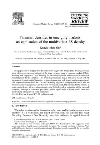
  • 17. 213I. Mauleon / Emerging Markets Review 4 (2003) 197–223´ Fig. 1. (a) ES density Singapore; (b) Gaussian density. Fig. 2. Bivariate density.
  • 18. 214 I. Mauleon / Emerging Markets Review 4 (2003) 197–223´ independently, (1) the correlation matrix, and, (2) the density and conditional variance parameters, according to expressions Eqs. (2.1) and (2.2), respectively, (i.e. the a ’s and the d ’s). All three estimated densities being estimated byi s maximum likelihood, do not yield negative values (precisely because this estimation method ensures that property; see the discussion below Eq. (2.1) in Section 2). This has been checked further, by solving the polynomial equation, {1q since there are no real solutions in any of the three cases,8 w x}d H (´ ) s0:is s it8ss2 the estimated densities can never become negative, either (this check has also been run on the estimated values in Tables 2 and 3). The typical shape for the estimated density is visualized and compared to the Gaussian (0, 1) in Fig. 1. Two of the most salient features of financial distributions are well captured (a high peak in the middle, and thick tails). Since all odd polynomials are non significant, no asymmetry is found in the series analysed. Table 2, in turn, presents the results of a simultaneous estimation of all parameters and the three equations, according to the ES Type I p.d.f. specification given in Eq. (3.8). This amounts to estimating a 32 parameters non-linear model. Since the model is highly non-linear, the task at first sight is daunting. However, and because of the relationship between marginal and joint densities explained in Eqs. (3.3) and (3.4), the results for the marginal densities of the form Eq. (2.1) estimated independently, can be taken as a starting point for the simultaneous estimation algorithm. Since the OLS estimation of Eq. (4.1) yields consistent estimates, as well, these values can also be taken as a starting point for the simultaneous estimation—and the same applies to the correlation matrix estimated in the first step from the OLS residuals of Eq. (4.1). All this greatly simplifies the task of estimating simultaneously all the 32 parameters i.e. Table 1 is the starting point for the optimization of Table 2. Finally, the method of Eq. (3.16) has been implemented to deal with the different sample sizes available for the data series. The estimation algorithms converge quickly without further complications. Turning now to the results of Table 2 themselves, the first to be noticed is the ability of the type of density analysed, that is, the ES density, to fit the data—at least in the sense that all the d coefficients are significant. In previous work (sees Mauleon (1997)), it was found that this density was able to fit most types of´ financial data—the stock market, interest and exchange rates, in developed financial markets. The results presented here, being obtained in emerging markets, enhance the applicability of the ES density. The second important result presented here, is the simultaneous estimation of the multivariate density for three equations and all the relevant parameters involved i.e. the conditional heteroskedasticity parameters, and the coefficients of the explanatory variables. This suggests the feasibility of estimating multivariate models of higher dimensionality, which may be rather useful in financial applications, and notably in the analysis of Value at Risk. Another result worth discussing can be drawn from the comparisons of parameter estimates under the two procedures—independently in Table 1, and simultaneously in Table 2. It is more or less immediate that the density and heteroskedasticity parameters stay basically invariant, but the correlation matrix and the coefficients of the explanatory
  • 19. 215I. Mauleon / Emerging Markets Review 4 (2003) 197–223´ variables change considerably, in some cases at least. One of the properties of the multivariate ES p.d.f. is that it can account for crossed effects beyond covariances. Here, coskewness and cokurtosis have been considered (see Eq. (3.7) in Section 3). The estimation results do not yield any significant coefficient in this case, though. This may be because the series are only weakly related, as evidenced by the low correlation values. Nevertheless, these crossed effects deserve further scrutiny in future empirical research. The shape of the joint density of Hungary and Singapore is visualised in Fig. 2. The results of estimating the ES Type II p.d.f. of Eq. (3.10) are presented in Table 3, and are commented briefly next. Similarly to the preceeding case, Table 1 can be taken as the starting point for the maximum likelihood non-linear estimation algorithm, and this smooths the whole estimation procedure that converges without further complications (in particular, and as pointed out in Eq. (3.9), the marginal densities are of the form Eq. (2.1), since the results of Eqs. (3.3) and (3.4) apply). This form of the density fits the data adequately, as in the previous case (at least in the sense that most coefficients are significant). Comparing the overall results to those of the ES Type I of Table 2, it is immediate that there are substantial changes in several parameter estimates. To some extent, this is just a reflection of the different functional forms. On the other hand, the results of the ES Type I in Table 2 seem to track more closely those obtained through independent estimation (see Table 1): this may suggest that the ES Type I is a better choice. Finally, it should also be kept in mind that the ES Type II, being obtained after deleting a cross product of the ES Type I, is a somewhat simpler analytical form than the ES Type I (compare Eq. (3.5) to Eq. (3.9)), and that uncorrelation does not imply independence, whereas it does with the ES type I. The results of estimating the ES Type III p.d.f. of Eq. (3.11) are presented in Table 4. This density may be specially useful when the maximum likelihood estimation method cannot be implemented or, simply, it is not the best solution for any other reason (see discussion in Section 2 on this point, and below Eq. (3.11) in Section 3). Estimates are presented in order to show the feasibility of this alternative density. Good starting values are provided by the estimated marginal densities, which are of the general form given in Eq. (2.1), but with restricted coefficients (see Eq. (A4)) in Appendix A; see also Eq. (A7) for the precise definition of the coefficients d in this case). Coskewness and cokurtosis have alsois been considered but are not significant. We note that the coefficients d and theis matrix R of Eq. (3.12) in this model do not mean strictly the same as in Table 2 and, therefore, are not directly comparable. The remaining coefficients do not change substantially in this specification. On balance, the broad conclusion might be that the ES Type I is to be recommended when the maximum likelihood estimation procedure can be imple- mented; when it cannot, or it is not advisable for any other reason, the ES Type III is available. We turn the focus, now, to the estimation of the Student’s t p.d.f. The results of estimating Student’s t densities are given in Table 5 (independently for every density), and Table 6 (the joint multivariate estimation). As pointed out in Section 3.2, the marginal densities of the multivariate Student’s t are themselves
  • 20. 216 I. Mauleon / Emerging Markets Review 4 (2003) 197–223´ distributed as t densities, but with a common value for the degrees of freedom: this feature suggests that marginal p.d.f. estimates (Table 5) may provide good starting values for the joint multivariate estimation (Table 6); but it also points to the main source causing the different estimation results: the value for the degrees of freedom in Table 6 turns out to be close to the averaged univariate degrees of freedom, weighted by the different available sample sizes. Since the variance depends on this value (the degrees of freedom), that may help explain why the estimated Garch processes change, substantially in some cases. Comparing these results to those obtained with the multivariate ES, one advantage of the multivariate t may be its relative simplicity; however, imposing a common value for the degrees of freedom may be too strict a restriction in some cases, or for some purposes. Other specific properties of the ES have already been discussed below Eq. (2.1), and in Eq. (3.7) Section 3.1 (see also Mauleon and Perote (2000), for a comparison in the univariate´ context). It should be pointed out, nevertheless, that the multivariate ES p.d.f. can account simultaneously for tail thickness and asymmetric behaviour—different for every marginal p.d.f., coskewness and cokurtosis. It is not yet clear how other multivariate p.d.f.’s can accomplish these same tasks. The main empirical results of this research can be summarized as follows: (1) the ES density performs well in financial markets of emerging economies, as well as in more developed economies, as shown in previous research (see Refs. in the Section 1), (2) it is feasible to estimate a multivariate ES density of large dimensionality. This feature makes the ES p.d.f. applicable, among others, to the problem of risk management in financial institutions, (3) independent estimation of the marginal densities, though being a consistent procedure, yields estimates significantly different from the multivariate estimation, at least for some parameters; this points to the superiority of the multivariate approach, (4) several types of multivariate densities have been proposed and estimated successfully in this research; among other properties, they can account for asymmetries, thick tails and outliers, and crossed effects beyond correlation, like coskewness and cokurtosis, (5) The different types have been compared, and their relative merits assessed, the general conclusion being that the ES type I may be the preferred choice in maximum likelihood estimation contexts, and the ES type III otherwise, (6) A final comparison with the multivariate t p.d.f. has been provided; in this respect, the conclusion may be that the ES is less restrictive, but at the cost of an increased complexity; in practice, this trade off may offer a guide as to the most suitable choice. 5. Summary and conclusions The purpose of this research has been to introduce the multivariate ES p.d.f., discuss its main theoretical properties, and apply it to the study of the characteristics of some financial markets in emerging economies. For that purpose, the exchange rate w.r.t. the US dollar of three countries from the main economically emerging zones have been selected—Chile for South America, Singapore for South East Asia, and Hungary, for the former Eastern block. The multivariate ES p.d.f. has been derived in a simple way from univariate results; several specific cases suitable for
  • 21. 217I. Mauleon / Emerging Markets Review 4 (2003) 197–223´ applied work have been proposed; they are devised to estimate the density in maximum likelihood contexts, as well as in other frameworks where this method- ology may not be suitable. The empirical work has involved estimating the ES density from this set of data in two ways, independently for each country, and simultaneously. Several special cases of the ES p.d.f. introduced in the paper have been fitted to the data. For the purposes of comparison, univariate and multivariate Student’s t p.d.f. have also been estimated. Other features of the models implemented are: (a) the Bollerslev (1990) model for the multivariate conditional heteroskedasticity, and (b) a vector autore- gressive model for the rate of change of the original variables i.e. the exchange rates of the three countries considered in the study. In all cases the estimation has been conducted by maximum likelihood. The multivariate estimation has involved the simultaneous estimation of a non-linear model with 32 parameters. For that purpose, the theoretical results relating marginal and multivariate p.d.f.’s have provided the starting points for the estimation algorithms, that converge without further difficulties. The main results of the empirical research can be summarized as follows: (1) The ES density performs well in financial markets of emerging economies, as well as in more developed economies, as shown in previous research (see Mauleon´ (1997) and Mauleon and Perote (2000)); (2) The multivariate ES p.d.f. presented´ in this paper performs well empirically, pointing to the feasibility of estimating multivariate ES p.d.f.’s of large dimensionality. This feature makes the ES p.d.f. applicable, among others, to the problem of risk management in financial institutions, (3) independent estimation of the marginal densities, though being a consistent procedure, yields significantly different estimates from the multivariate estimation, at least for some parameters; this is in spite of the moderately large sample size, and the fact that independent estimation of the main blocks of parameters involved is consistent asymptotically, and points to the superiority of the multivariate approach, (4) several types of multivariate densities, appropriate in different frameworks, have been proposed and estimated successfully in this research; among other properties, they can account for asymmetries, thick tails and outliers, and crossed effects beyond correlation, like coskewness and cokurtosis, (5) the different types of multivariate ES p.d.f. introduced in Section 3 of the paper have been compared, and their relative merits assessed, with the general conclusion that the ES type I may be the preferred choice in maximum likelihood estimation contexts, and the ES type III otherwise, (6) A final comparison with the multivariate Student’s t p.d.f. suggests that the ES p.d.f. is less restrictive, and able to account for several departures from Normality empirically relevant; this, however, comes at the cost of an increased complexity, and the appropriate practical choice may depend on this trade off. Estimating the densities of financial series is a major research topic in applied finance research, and the results of this paper are a contribution to that field. They also suggest that the ES density may be fully applicable to other realistic problems (such as risk management in financial institutions). Coupled with other developments
  • 22. 218 I. Mauleon / Emerging Markets Review 4 (2003) 197–223´ (see Mauleon (1999)), they point to the analytical and practical capabilities of the´ family of multivariate ES p.d.f. analysed in this paper. Appendix A: Restrictions to ensure a non negative ES p.d.f. This appendix provides a sufficient set of conditions that ensure that the ES p.d.f. is always non negative. The restrictions are obtained through a squared transforma- tion of the basic sum of weighted Hermite polynomials. Sections 1 and 2 discuss the univariate case, and show how the squared transformation can be rewritten as a standard ES p.d.f. density, but with restricted weights; Section 3 provides a multivariate generalization. Section 1 It is convenient to start by noting that, since the H (´ ) are polynomials of degrees it s on ´ , their weighted sum in Eq. (2.1) can also be written alternatively as a sumit of powers on ´ , that is,it q q s d H ´ s g ´ , (A1)Ž .s s it s it8 8 ss0 ss0 where are the (qq1) vectors of the g , and the d , respectively, ™ ™™ ™gsC d, g and dq s s and C, is a (qq1)x(qq1) squared non singular matrix of known constants (see Kendall and Stuart (1977); note that d s1, H s1, g /1).0 0 0 Let us consider now, the following p.d.f., obtained through a squared transfor- mation of a polynomial of the type Eq. (A1): q 2w zB E U U s f ´ sa ´ g q g ´ . (A2)C FŽ . Ž .x |it it 0 s it8D Gy ~ss0 The parameter g * can be adjusted to ensure that the probability integral is unity,0 i.e. If we can ensure that 0-g *, as well, then f(´ )00, so that q` f(´ )s1.it 0 it|y` f(´ ) is a well-defined p.d.f. for any set of {g *} values. Section 2 discusses howit s to achieve this, and explains the relationship between both set of parameters (the {g *} and the {g }).s s Let us develop, now, the squared transformation of Eq. (A2), i.e. q q 2qw z w z U U U Usqr n f ´ sa ´ g q g g ´ sa ´ g q f ´ , (A3)Ž . Ž . Ž .x | x |it it 0 s r it it 0 n it88 8y ~ y ~rs0ss0 ss0 where By the same token as in Eq. (A1), we can rewrite theU Unf s g g .n s nys8ss0 polynomial on ´ , as a weighted sum of Hermite polynomials, i.e.it
  • 23. 219I. Mauleon / Emerging Markets Review 4 (2003) 197–223´ 2qw z f ´ sa ´ 1q c H ´ , (A4)Ž . Ž . Ž .x |it it s s it8y ~ss1 where (note that are all of order (2qq1)). Since the ™ ™™ ™y1 csC f c, f, C ,2q 2q probability integral is unity, the integral of the Hermite polynomials times a N(0, 1) p.d.f. between (y`, q`) vanish (see Appendix B), and H (´ )s1, then it0 it must also be that c s1yg *, and the leading constant in the polynomial of Eq.0 0 (A4) becomes 1, as stated. Notice, finally, that the restricted coefficients c , (sss 1,«, 2q) depend on the unrestricted d ,(ss1,«, q) (see Eq. (A5)), so that theres are q restrictions embodied in the set cs. Section 2 We start by considering the squared of the transformation of Eq. (A1), i.e. q 2 q 2B E B E s d H ´ s g ´ , (A5)C F C FŽ .s s it s it8 8D G D Gss0 ss0 where d s1, to ensure that the original polynomials are kept in the squared0 transformation. Let us define now, the constant u, by, q` q 2w zB E s us a ´ 1q g ´ d´ . (A6)C FŽ .x |it s it it| 8D Gy ~y` ss0 By means of the orthogonality property of Hermite polynomials, it can be shown that, (see Kendall and Stuart (1977)). Then, and from Eqs. (A5)2qus2q d s!s8ss0 and (A6), the following function is a well defined p.d.f., q 2w zB E y1 f ´ su a ´ 1q d H ´ , (A7)C FŽ . Ž . Ž .x |it it s s it8D Gy ~ss0 since it is always non negative, and the probability integral is one. Substituting Eq. (A5) again, this can also be written as, q 2w zB E U U s f ´ sa ´ g q g ´ , (A8)C FŽ . Ž .x |it it 0 s it8D Gy ~ss0 where g *s1yu, g *sg yu which is the expression of Eq. (A2). We finally1y2 0 s s note that since 1-u, then 0-g *-1 as required (see discussion following Eq.0 (A2)). Section 3 Let us write first the density of Eq. (A4) as follows (note that we do not substitute c ),0
  • 24. 220 I. Mauleon / Emerging Markets Review 4 (2003) 197–223´ 2qw z U w zx | f ´ sa ´ g q c H ´ sa ´ vqQ ´ , (A9)Ž . Ž . Ž . Ž . Ž .x |it it 0 s s it it ity ~8y ~ss0 where by construction vsg *)0, Q(´ )00 (this has been proved in Sections 10 it and 2 above). This is just a notational simplification introduced for the sake of clarity in what follows. We define now, the bivariate density by a straightforward multiplication of two independent ES densities as given in Eq. (A9), and rearrange the result as follows: w zw zx |x | f ´ f ´ sa ´ a ´ v qQ ´ v qQ ´Ž . Ž . Ž . Ž . Ž . Ž .1t 2t 1t 2t 1 1 1t 2 2 2ty ~y ~ sa ´ a ´ v vŽ . Ž .1t 2t 1 2 w zw zx |x | qa ´ a ´ v qQ ´ v qQ ´ yv v , (A10)Ž . Ž . Ž . Ž .1t 2t 1 1 1t 2 2 2t 1 2µ ∂y ~y ~ where, again by construction, the term inside {Ø} in the second summation is non negative. Replacing the leading term a(´ )a(´ ) by a bivariate Gaussian density1t 2t with covariance matrix R, denoted by b(Ø), yields, f ´ ,´ sb ´ ,´ v vŽ . Ž .1t 2t 1t 2t 1 2 w zw zx |x | qa ´ a ´ v qQ ´ v qQ ´ yv v . (A11)Ž . Ž . Ž . Ž .1t 2t 1 1 1t 2 2 2t 1 2µ ∂y ~y ~ It is immediate now that f(´ , ´ )00, and the probability integral is one as1t 2t required for a well defined p.d.f. It is worth noticing, as well, that the marginal densities are as given in Eq. (A9), and that the covariance matrix is defined by, E ´ ´ sv v R , (A12)Ž .it jt i j ij where in order to achieve scale normalization, and without loss of generality, R sii 1 (this holds only when C s0 for both marginal p.d.f.’s; a sufficient condition is1 that all odd d in Eq. (A7) vanish, so that the density is symmetric). Thes generalization to n variates is immediate, leading to, n n 2qw zw zS W T T U Xf ´ sWb ´ q a ´ v q c H ´ yW , (A13)Ž . Ž . Ž . Ž .x |x |t t it i is s itT T2 2 8V Yy ~y ~is1 is1 ss0 where (this is the expression Eq. (3.11) in Section 3.1). The marginalnWs vi2is1 densities are as given in Eq. (A9), and, as explained in Sections 1 and 2, the parameters c , (ss0,«, 2q) are functions of the parameters d , (ss0,«, q).is is Notice, finally, that it is this latter set of unrestricted parameters that is reported in Table 4. Appendix B: Results on Hermite polynomials Since the polynomials are defined by the identity D a(´ )s(y1) a(´ )H (´ )s s it it s it (see Section 1 of the main text), it is immediate that,
  • 25. 221I. Mauleon / Emerging Markets Review 4 (2003) 197–223´ s sy1 y1 a ´ H ´ d´ sD a ´ , s01, (A14)Ž . Ž . Ž . Ž .it s it it it| with the convention D a(´ )sa(´ ). Now and since D a(´ )™0, as ´ ™"`,0 s it it it it s00, it follows that the integral of Eq. (A14), in the space (y`, q`) vanishes. It is also convenient to note that a general expression for the Hermite polynomials exists in closed form, and is given by, w x2rsy2 sr sy2r H ´ s (y1) ´ , (A15)Ž .s it it8 r 2 r!rs0 where s s(s(sy1)(sy2)«(sy2rq1)), and rs0,«, (wsy1xy2) if s is odd (seew x2r Abramowitz and Stegun (1972) and Kendall and Stuart (1977)). References Abramowitz, M., Stegun, I., 1972. Handbook of mathematical functions. Dover, New York. Aıt-Sahalia, Y., Lo, A., 1998. Non parametric estimation of state-price densities implicit in financial¨ asset prices. J. Finance 53, 499–547. Akgiray, V., Booth, G., 1988. Mixed diffusion-jump process modeling of exchange rate movements. Rev. Econ. Stat. 70, 631–637. Anderson, T.W., 1984. An Introduction to Multivariate Statistical Analysis. second ed. Wiley & Sons. Ang, A., Chen, J., Xing, Y., 2002. Downside Risk and the Momentum Effect, Columbia Business School, working paper. Aparicio, J., Estrada, J., 2001. Empirical distributions of stock returns: European securities markets, 1990–95. Eur. J. Finance 7, 1–21. Ball, C., Roma, A., 1993. A jump diffusion model for the European monetary system. J. Int. Money Finance 12, 475–492. Ball, C., Torous, W., 1983. A simplified jump process for common stocks returns. J. Financ. Quant. Analysis 18, 53–65. Barton, D.E., Dennis, K.E., 1952. The conditions under which Gram-Charlier and Edgeworth curves are positive definite and unimodal. Biometrika 39, 425–427. Bernardo, J., Smith, A.F., 1994. Bayesian Theory. Wiley & Sons. Blattberg, R., Gonedes, N., 1974. A comparison of the stable and student distributions as statistical model for stock prices. J. Business 47, 244–280. Bekaert, G., Erb, C., Harvey, C., Viskanta, T., 1998. Distributional characteristics of emerging market returns and asset allocation. J. Portfolio Manage. winter, 102–116. Bollerslev, T., 1990. Modelling the coherence in short-run nominal exchange rates: a multivariate generalized ARCH model. Rev. Econ. Statist. 72, 498–505. Bollerslev, T., Engle, R.F., Nelson, D.B., 1994. ARCH Models. In: Engle, R., McFadden, D. (Eds.), Handbook of Econometrics, Vol. 4. Elsevier Science BV, Amsterdam. Bourgoin, F., Prieul, D., 1997. Estimation de Diffusion a volatilite Stochastique et Application au Taux` ´ d’Interet a Court Terme Francais, presented at the Forecasting Financial Markets Conference, convened´ ˆ ` jointly by the Imperial College and the BNP, London. Britten-Jones, M., Schaefer, S., 1999. Non-linear Value-at-Risk. Eur. Finance Rev. 2 (2). Dowd, K., 1998. Beyond Value at Risk. John Wiley & Sons. Duffie, D., Pan, J., 1997. An overview of Value at Risk. J. Derivatives 4 (3), 9–49. Erb, C., Harvey, C., Viskanta, T., 1994. Forecasting international equity correlations. Financ. Analysts J. November, 32–45.
  • 26. 222 I. Mauleon / Emerging Markets Review 4 (2003) 197–223´ Gallant, R., Fenton, V., 1996. Convergence rates of SNP density estimators, mimeo, University of North Carolina. Gallant, R., Nychka, D., 1987. Seminonparametric maximum likelihood estimation. Econometrica 55, 363–390. Gallant, R., Tauchen, G., 1989. Seminonparametric estimation of conditionally constrained heterogeneous processes: asset pricing applications. Econometrica 57, 1091–1120. Goodhart, C., O’Hara, M., 1997. High frequency data in financial markets: issues and applications. J. Empirical Finance 4, 73–114. Gray, B., French, D., 1990. Empirical comparisons of distributional models for stock index returns. J. Business Finance Account. 17, 451–459. Hamilton, J., 1991. A Quasi-Bayesian approach to estimating parameters for mixtures of normal distributions. J. Business Econ. Stat. 9, 27–39. Hansen, B., 1994. Autoregressive conditional density estimation. Int. Econ. Rev. 35 (3), 705–730. Harvey, C., Siddique, A., 1999. Autoregressive conditional skewness. J. Financ. Quant. Anal. 34 (4), 465–488. Harvey, C., Siddique, A., 2000. Conditional skewness in asset pricing tests. J. Finance 55 (3), 1263–1295. Harvey, C., Zhou, G., 1993. International asset pricing with alternative distributional specifications. J. Empirical Finance 1, 107–131. Jorion, P., 1988. On jump processes in the foreign exchange and stock markets. Rev. Financ. Studies 1, 427–445. Kendall, M., Stuart, A., 1977. The Advanced Theory of Statistics. fourth ed. Griffin & Co, London. Lamoureux, Ch., Lastrapes, W., 1990. Persistence in variance, structural change, and the GARCH model. J. Business Econ. Stat. 8 (2), 225–234. Leamer, E., 1978. Specification Searches. Wiley & Sons. Longin, F., Solnik, B., 2001. Extreme correlations of international equity markets. J. Finance LVI (2), 649–676. Mauleon, I., 1983. Approximations to the Finite Sample Distribution of Econometric Chi-Squared´ Criteria, unpublished Ph.D. dissertation, London School of Economics. Mauleon, I., 1997. Long memory in conditional variances: a new and stable model. J. de la Societe de´ Statistique de Paris 138 (4), 67–88. Mauleon, I., 1999. Testing Forecasting Stability under non Gaussianity, (mimeo) International Sympo-´ sium on Forecasting 99, Washington DC. Mauleon, I., Perote, I., 2000. Testing densities with financial data: an empirical comparison of the´ Edgeworth–Sargan density to the Student’s t. Eur. J. Finance 6, 225–239. McDonald, J.B., Newey, W.K., 1988. Partially adaptive estimation of regression models via the generalized t distribution. Econometric Theory 4, 428–457. McDonald, J., Xu, Y., 1995. A generalization of the beta distribution with applications. J. Econometrics 66, 133–152. Nelson, D., 1991. Conditional heteroskedasticity in asset returns: a new approach. Econometrica 59, 347–370. Pagan, A., Schwertz, W., 1990. Testing for covariance stationary in stock market data. Econ. Lett. 33, 165–170. Pagan, A., Schwertz, W., 1990. Alternative models for conditional stock volatility. J. Econometrics 45, 267–290. Perote, J., 1999. Fitting densities to financial data, unpublished Ph.D. dissertation, University of Salamanca. Phillips, P., Loretan, M., 1994. Testing the covariance stationarity of heavy-tailed time series. J. Empirical Finance 1, 211–248. Phillips, P., 1995. On the theory of testing covariance stationarity under moment condition failure. In: Maddala, G., Phillips, P., Srinivasan, T. (Eds.), Advances in Econometric and Quantitative Economics. Blackwell, Oxford, pp. 198–233.
  • 27. 223I. Mauleon / Emerging Markets Review 4 (2003) 197–223´ Praetz, P., 1972. The distribution of share price changes. J. Business 45, 49–55. Prucha, I., Kelejian, H., 1984. The structure of simultaneous equation estimators: a generalization towards nonnormal disturbances. Econometrica 52, 721–737. Rogalski, R., Vinso, J., 1978. Empirical properties of foreign exchange rates. J. Int. Business Studies 9, 69–79. Sargan, J.D., 1976. Econometric estimators and the Edgeworth approximation. Econometrica 44, 421–448. Sargan, J.D., 1980. Some approximations to the distribution of econometric criteria which are asymptotically distributed as chi-squared. Econometrica 48, 1107–1138. Shenton, L.R., 1951. Efficiency of the method of moments and the Gram-Charlier type a distribution. Biometrika 38, 58–73. Silverman, B.W., 1986. Density estimation for statistics and data analysis. Chapman & Hall, London. Vlaar, P., Palm, F., 1993. The message in weekly exchange rates, in, the European monetary system: mean reversion, conditional heteroskedasticity and jumps. J. Business Econ. Stat. 11, 351–360. Zhou, G., 1993. Asset pricing tests under alternative distributions. J. Finance 48, 1927–1942.