Best VIP Call Girls Morni Hills Just Click Me 6367492432
Abad thore in managerial & decision economics
1. MANAGERIAL AND DECISION ECONOMICS
Manage. Decis. Econ. 25: 231–241 (2004)
Published online 16 June 2004 in Wiley InterScience (www.interscience.wiley.com). DOI: 10.1002/mde.1145
Fundamental Analysis of Stocks by
Two-stage DEA
Cristina Abada,*, Sten A. Thoreb and Joaquina Laffargaa
a
Universidad de Sevilla, Sevilla, Spain
b
The University of Texas at Austin, USA
Fundamental analysis of stocks links financial data to firm value in two consecutive steps: a
predictive information link tying current financial data to future earnings, and a valuation link
tying future earnings to firm value. At each step, a large number of causal factors have to be
factored into the evaluation. To effect these calculations, we propose a new two-stage multi-
criteria procedure, drawing on the techniques of data envelopment analysis. At each stage, a
piecewise linear efficiency frontier is fitted to the observed data. The procedure is illustrated by
a numerical example, analyzing some 30 stocks in the Spanish manufacturing industry in the
years 1991–1996. Copyright # 2004 John Wiley & Sons, Ltd.
INTRODUCTION that fundamental analysis is predictive, examining
information from financial statements (the finan-
Fundamental analysis of stocks (for references, see cial ‘fundamentals’ of a stock) and generating a
next section below) determines the ‘fundamental’ forecast of its market value. This is the applica-
value of a stock by analyzing available informa- tion, no doubt, that most authors on the subject
tion with a special emphasis on accounting have had in mind. Another, and quite different
information. Over the last decade, accounting interpretation that will occupy us presently, is
researchers have redirected their attention to this normative. Adopting this perspective, and again
task. A number of empirical studies have used inspecting the financial fundamentals of a stock,
information from financial statements to predict we shall calculate the market value that the stock
future earnings as an indication of the future ‘should’ (or ‘could’) fetch under some carefully
performance of a firm. Next, the market evalua- spelled-out circumstances of optimal management
tion of this future earnings-potential is assessed. and optimal market valuation. For those few
Comparing with the actual price, the analyst corporations that are well managed and well
identifies stocks that are overvalued or under- understood by the stock market, this normative
valued. The undervalued ones are candidates for value will indeed serve as realistic market forecast.
investment and would hopefully earn ‘abnormal’ Most corporations, however, will fall short of
returns. Most of these studies use econometric these idealized circumstances. The normative value
techniques to process the information contained in will then exceed the actual market performance.
the financial statements. The present paper pro- To use a term that will be important in the
poses an alternative methodological approach. following, the normative value is in the nature of
Fundamental analysis can essentially be under- an idealized ‘efficiency frontier’ that a few stocks
stood in two different ways. One interpretation is will attain but most stocks will linger behind.
Fundamental analysis of stocks proceeds in two
steps. The first step inspects the financial data of a
*Correspondence to: Departamento de Contabilidad y Econ-
omia Financiera, Universidad de Sevilla, Avda. Ramon y Cajal, corporation } its profit-and-loss account and
1, 41018, Sevilla, Spain. E-mail: cabad@us.es its balance sheet } and aims at assessing future
Copyright # 2004 John Wiley & Sons, Ltd.
2. 232 C. ABAD ET AL.
earnings. The second step traces the causal link each stock, the idealized and unobserved revenues
from future earnings to market value. For both of calculated from the first frontier are fed as inputs
these two steps, we shall adopt a normative into the second frontier.
interpretation. First, we shall calculate an effi- Following section reviews the fundamental
ciency frontier that traces the idealized relation- analysis approach to stock valuation. Next section
ship between standard financial indicators and presents the mathematical developments. Follow-
revenues. Stocks at the frontier are optimally well ing this, we report on the data and on the results of
managed, converting the various financial inputs an illustrative numerical example } the two-stage
into maximal revenues. Stocks falling behind the DEA model is estimated for a sample of firms
frontier are less well managed. Second, we shall quoted on the Madrid Stock Exchange. Final
calculate an efficiency frontier that traces an section sums up.
idealized relationship between various financial
data and market value. Stocks at the frontier are
optimally priced in the market. Stocks falling
behind the frontier are valued less favorably. REVIEW OF FUNDAMENTAL ANALYSIS
To calculate these frontiers numerically, we shall RESEARCH}STRUCTURING THE
make use of a technique called ‘data envelopment FUNDAMENTAL ANALYSIS APPROACH TO
analysis’ or DEA, for short. It was pioneered by STOCK VALUATION AS A TWO-STAGE
Charnes, Cooper and Rhodes in 1978 (for a recent CAUSAL PROCESS
comprehensive treatment, see Charnes et al., 1994)
and fits a piecewise linear envelope or ‘frontier’ to In the 1970s and 1980s, capital markets accounting
the given data. The basic idea is easy to explain. research focused on the study of stock market
Given a collection of points in a multidimensional response to the disclosure of accounting informa-
space, DEA calculates its upper convex hull or tion, under the assumption of market efficiency.
‘envelope’. Thus, representing each stock as a More recently, some authors have questioned the
point in a multidimensional space, DEA will validity of the market efficiency hypothesis either
calculate an envelope frontier to the stocks. The because it seemed to yield inconclusive results
frontier indicates a normative ideal. Stocks located (Lev, 1989) or because anomalies in market
at the frontier are optimally adjusted. Stocks behavior were detected (Ball, 1992). Efficiency
below the frontier are sub-optimally adjusted. implies that the market price is a good estimate of
For the use of DEA to analyze corporate financial intrinsic value. Questioning efficiency, a door is
data, see Thore et al. (1994), Thore et al. (1996) opened to the possibility that the price does not
and Thore (1996). well reflect intrinsic value. In this setting, the
A characteristic feature of fundamental analysis objective of fundamental analysis is to determine
is that it searches for an explanation of stock price whether or not current stock prices fully and
and market value via an un-observed underlying instantaneously incorporate information about
causal factor: future earnings. Precisely because it future earnings (or other future economic vari-
is un-observed, fundamental analysis searches ables) contained in the fundamental variables (i.e.
deeper, down to the financial fundamentals of current prices approximate intrinsic or fundamen-
the stock. The last step of fundamental analysis tal value).
(associating future earnings with market value) Fundamental analysis typically uses econo-
therefore can never stand on its own. It needs the metric techniques like logit/probit analysis
preceding first step as a prerequisite (associating (Ou and Penman, 1989; Holthausen and Larcker,
standard financial indicators of the stock with 1992; Stober, 1992; Greig, 1992; Bernard et al.,
future earnings). 1997; Setiono and Strong, 1998; Charitou and
To represent this cascading causal mechanism Panagiotides, 1999; Beneish et al., 2001) or
mathematically, we propose a novel format of regression analysis (Lev and Thiagarajan, 1993;
the so-called two-stage DEA. We construct two Abarbanell and Bushee, 1997; Sloan, 1996). In
successive DEA frontiers fitted to the statistical order to assess the extent to which stock prices
observations, with revenues being an output reflect information about future earnings con-
variable of the first frontier, and an input variable tained in current financial statement data, a test
into the second frontier. To be more precise: for developed by Mishkin (1983) was later applied by
Copyright # 2004 John Wiley & Sons, Ltd. Manage. Decis. Econ. 25: 231–241 (2004)
3. FUNDAMENTAL ANALYSIS OF STOCKS 233
a series of authors (see Sloan (1996), Collins and Although future dividends or future cash flows
Hribar (2000), Thomas (2000), Beaver and McNi- are usually employed to approximate those
chols (2001), and Xie (2001)). Results from these unobserved attributes, Ou suggested that future
studies seem to indicate that stock prices do not earnings are value-relevant as well } see Ou
fully reflect information about future earnings and Penman (1989), Stober (1992), Setiono and
contained in financial information. The conclusion Strong (1998), Charitou and Panagiotides (1999),
would then follow that the market is inefficient and others, indicating that investors may have
with respect to certain financial statements data. the possibility of using publicly available financial
Assuming that the stock market is not fully able statements information mechanically, applied
to process the information contained in the uniformly across companies, to predict subsequent
financial statements, so that market prices deviate earnings changes. To sum up the argument,
from fundamental values, suitable investment Ou provided evidence that, in terms of
strategies can then be designed. Several authors financial statements analysis, the relation-
have indeed claimed that market prices do not ship between financial data and firm value
instantaneously incorporate all the relevant in- is established through a two-stage causal
formation contained in the financial statements, process:
and that ‘abnormal returns’ can be generated (see * a predictive information link that ties current
Ou and Penman (1989), Stober (1992), Holthausen
financial data to projected future earnings, and
and Larcker (1992), Abarbanell and Bushee * a valuation link that ties projected future
(1998), Sloan (1996), Collins and Hribar (2000),
earnings to firm value.
Thomas (2000), and Xie (2001)).
Our own approach differs from the econometric Following Ou, then, the purpose of fundamental
estimation employed in all previous studies. We analysis is to identify hidden or implied causal
shall use DEA to rank firms on the basis of factors drawn from financial accounting data that
accounting information. One of the main advan- can be used to explain the market value of the
tages of this approach is that the valuation exercise stock. For our present purposes, we shall assume a
is made in a comparative fashion: DEA compares chain of causation as follows:
stocks to each other in order to determine their
Financial accounting data ) Projected earnings
relative efficiency, rather than examining each
stock individually. Stocks need to be compared ) Market value:
to each other, before the analyst can decide which In this causal process, the factor ‘projected
one offers the best investment opportunities. earnings’ is an intermediary causal factor. It is at
the same time the estimated output of
Structuring the Fundamental Analysis Approach to the predictive information link (Financial accoun-
Stock Valuation as a Two-Stage Causal Process ting data ! Projected earnings), and the input
into the valuation link (Projected earnings ! Market
According to Ou (1990, p. 145), the observed value). Thus, the valuation link cannot be esta-
association between accounting information and blished separately, without first estimating Pro-
stock market value is the result of (i) a link between jected earnings.
accounting information and future streams of A couple of elementary accounting relations
benefits from equity investments, and (ii) a valua- may be invoked to identify the two links. First,
tion link between future benefits and stock market and simplifying, write the Market Value of a
values. The disclosure of new accounting informa- corporation as a function of Book Value and
tion may lead to revisions of investor expectations Operating Income.
about future benefits and to corresponding adjust-
ments in current market value. Market Value ¼ f ðBook Value; Operating IncomeÞ:
This implies that the documented association Given that Operating Income equals Reve-
between accounting information and stock prices nues minus Operating Expenses, this can also be
or stock returns can be understood as the result of written as
a link (the predictive information link) between
Market Value ¼ f ðBook value; Revenues;
accounting information and certain value-relevant
unobservable attributes. Operating ExpensesÞ:
Copyright # 2004 John Wiley & Sons, Ltd. Manage. Decis. Econ. 25: 231–241 (2004)
4. 234 C. ABAD ET AL.
Given this, our aim in the first stage will be to use operations of the firm (i.e. needed for generating
information contained in financial statements revenues).
ratios in order to project Revenues. Plugging The valuation link. How does the market
during the second stage this projection into the translate future earnings into stock value? Accor-
function f ð Þ above, together with Operating ding to the so-called residual income valuation
Expenses and Book Value, the model finally model (Ohlson, 1995), firm value is expressed as a
projects Market Value. function of both the book value of equity and the
As already mentioned, the present work does present value of future ‘abnormal earnings.’
not deal with the task of predicting market value, Feltham and Ohlson (1995) showed that operating
nor future earnings. Our concern is normative activities might yield abnormal earnings; hence, an
rather than predictive. understanding of firm value requires a forecast of
The predictive information link. Our aim is to future operating profitability (see also Fairfield
evaluate the efficiency of management in generat- and Yohn, 2001).
ing maximal revenues. As recognized by Graham Penman (1998) analyzed how book value and
and Dodd (1962), fundamental analysis is a long- earnings combine to determine stock value. To
term oriented exercise, where the management him, ‘future earnings are related to current book
factor plays an essential role: values, as well as current earnings, by the
intertemporal properties of accounting’ (Penman,
Over the long term, forecasting increasingly
1998, p. 294). In this manner, he argued, it would
depends on a correct appraisal of the compe-
be possible to arrive at a rough determination of
tence and integrity of management. The com-
the value of a stock without conducting a full pro
pany’s record demonstrates what ongoing
forma accounting analysis.
management has accomplished and is the
In our case, we shall assume that the value of the
primary source of judgment about the quality
firm is a function of earnings from operations
of management (ibid., p. 524).
(revenues and operating expenses) and of the book
Well-managed companies are more likely to value of equity:
keep generating a steady stream of revenues in the
future as well. Hence, there is a link between the
INPUTS:
past and current record of a company, and its Projected Revenues
future earnings prospects. Operating Expenses
To project Revenues we conventionally assume Book Value
that the firm aims at maximizing revenues given OUTPUTS:
its available resources. To characterize these Market Capitalization
inputs and outputs we use information from the
balance sheet and from the income statement. Projected Revenues and Operating Expenses
Specifically, we have used the following inputs and determine earnings generated during the current
outputs: period. Earnings not paid to shareholders remain
in the firm as retained earnings. The Book Value
variable accounts for retained earnings accumu-
INPUTS:
lated in the past.
Accounts receivables
Inventory Additionally, one may want to use one
Fixed assets or several indicators of price risk as an input
Other assets at this stage (such as the beta coefficient of the
Operating expenses stock).
OUTPUT:
Revenues
A CUMULATIVE TWO-STAGE DEA MODEL
The inputs account for the economic structure
used in the business (‘accounts receivables’, For the estimation of the input–output relation-
‘inventory’, ‘fixed assets’ and ‘other assets’) and ships outlined in the preceding section we for-
for other factors (‘operating expenses’) that mulate a two-stage DEA model. For extensive
account for the expenses incurred in running the discussions of two-stage DEA, see Charnes et al.
Copyright # 2004 John Wiley & Sons, Ltd. Manage. Decis. Econ. 25: 231–241 (2004)
5. FUNDAMENTAL ANALYSIS OF STOCKS 235
(1994) and Sexton and Lewis (2000). Whereas inefficiency in the valuation link does not mean
conventional two-stage DEA breaks up into two that markets are inefficient. Our analysis does not
separate consecutive steps that are estimated violate standard assumptions of the efficiency of
separately, our new procedure feeds the projected financial markets.
output of the first step as an input into the second The model format developed in the present
step. paper employs two consecutive DEA models, one
Efficiency in DEA refers to the efficiency (or for the predictive information link and one for the
inefficiency) of a manager to reach the boundary valuation link. The two stages are cumulative in
of his production set (the set of feasible production the sense that the outputs from the first link are fed
points). The production set of the predictive as inputs into the second one. In this manner, the
information link is simply an extended classical explanation of stock prices is established through a
production function, tying sales of a corporation two-stage process where the immediate causal
to its inputs like accounts receivables, other factors explaining stock prices actually are un-
assets and operating expenses. The DEA frontier observed, but instead calculated from an earlier
traces the geometrical locus of all Pareto-optimal DEA optimization process.
points of the production set. The piece-wise For both links, we shall use the so-called output-
linear frontier is said to be ‘spanned’ by its corner oriented version of DEA. For any given vector of
points, each such corner point representing an inputs, this version calculates the maximal array of
observed corporation that is rated as efficient. outputs that can be obtained. The purpose of the
Those corporations exhibit ‘best practice’ in the predictive information link is to project the
industry}the management of those corporations revenues of the company in absolute amounts,
that are able to convert the given inputs into given current accounting information on Accounts
the desired outputs more efficiently. Corporations receivables, Inventory, Fixed assets, Other assets,
falling behind the frontier are less efficiently and Operating expenses. For the valuation link,
operated. The DEA efficiency rating for given Projected Revenues and given Operating
the predictive information link thus provides Expenses and Book Value, the model calculates
a numerical measure of the aptitude of the the maximal Market Capitalization.
management team. In both stages, we allow for the possibility of
The production set of the valuation link has to variable returns to scale and, hence, the BCC
be understood in the attenuated sense of a model of DEA will be used (Banker et al., 1984).
general input–output relationship, not necessarily To sum up, the objective of the two-stage DEA
dealing with physical production. Such similes model is to determine the Pareto-optimal stock
are standard in the DEA literature. In the present price of each company that would take hold if
case, it relates the Projected Revenues, Operating (i) management were as able as that of the best-
Expenses and the Book Value of equity to managed companies in the industry, and (ii) the
the Market Capitalization of the firm stock. market were willing to accord the stock a price as
Again, the frontier will represent ‘best practice’ high as that accorded to the highest flyers in the
in the industry } the management of those market.
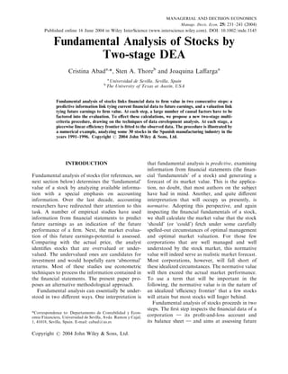
corporations that are able to translate a set of Geometric illustration. We have illustrated the
given financial data into the greatest values in the two-stage procedure schematically in Figure 1.
stock market. The figure features three axes: a first-stage input X,
For this link as well, efficiency may be tied to a first-stage output (second-stage input) Y, and a
management aptitude. Some CEOs are more able second-stage output Z. Events during the first
to time the product development and promotion stage are illustrated in the southeast quadrant of
activities of their corporation more cleverly than the diagram; events during the second stage are
others, creating favorable press coverage and illustrated in the northeast quadrant. We have
favorable expectations among the community of plotted two observations, A and B.
investment analysts. (Witness the current dot.com The first observation is represented as A1 in the
mania lifting the stock prices of IPOS to the skies, first-stage quadrant, and as A2 in the second
sometimes even in the absence of both sales and quadrant. A happens to lie on both the first-stage
profits.) Corporations falling behind the fron- frontier and the second-stage frontier. (The two
tier are run by less genial managers. However, frontiers have been drawn with thick lines). The
Copyright # 2004 John Wiley & Sons, Ltd. Manage. Decis. Econ. 25: 231–241 (2004)
6. 236 C. ABAD ET AL.
B3 B5 For the first stage, consider the output-oriented
variable Z
BCC model
A2
Maximize c
B2
subject to cYk0 À Sj lj Ykj 40; k 2 K1 ;
Sj lj Xij 4Xi0 ; i ¼ 1; 2; . . . m; ð1Þ
Sj lj ¼ 1;
lj 50; j ¼ 1; . . . n:
variable Y
In the interest of simplicity and expositional
A1
clarity, we do not exhibit the slacks in the
constraints explicitly. For the numerical calcula-
tions reported later, corresponding non-Archime-
dean formulations were actually employed.
Remember that the fundamentals of the first
B1 B4
variable X stage provide a kind of ‘hidden’ explanation of the
stock valuation in the second stage that the
Figure 1. Two-stage DEA procedures illustrated. second-stage variables alone cannot generate. That
See the text. is indeed the very essence of the idea of the stock
‘fundamentals.’ In order to explain the stock
valuation it just is not enough to look at the
second observation B is represented as B1 in the second-stage stock characteristics. One needs to
first-stage quadrant, and as B2 in the second-stage dig deeper in the causal structure, uncovering the
quadrant. This observation is inefficient at both underlying first-stage accounting performance.
stages. To accomplish this cumulative explanation from
Following the procedures of conventional the first stage to the second, we propose a novel
two-stage output-oriented DEA, the two obser- feature, feeding the projected outputs from the first
vations would be projected on the frontiers stage as inputs into the second stage. Using Fig. 1 as
as follows. For the first stage, A1 is already an illustration again, we now feed the first-period
located on the frontier and B1 projects onto point projected output of the B-observation as the input
B4. For the second stage, A2 is also already into the second stage. That is, we feed the input
located on the frontier while B2 would be of B4 into the second stage, and the projected
projected onto point B3. result is B5.
Mathematical notation: There are j ¼ 1; . . . ; n Turning to the general case and the mathema-
stocks. For each stock j, the inputs into the tical treatment, note that the projected outputs of
first stage Xij ; i ¼ 1; . . . ; m and the outputs the first-stage program (1) are
from the first stage Ykj ; k 2 K1 & K are re- Y à ¼ S là Y ; k 2 K ;
k0 j j kj 1
corded. (The index k runs over all elements in
the set K1 ; which is the set of all outputs from the where the asterisk denotes the optimal solution to
first stage.) program (1). Next, we feed these projected outputs
The inputs into the second stage are written as inputs into the second-stage program (2)
Ykj ; k 2 K2 & K: (This time, the index k runs Maximize c
over the elements of the set K2 ; which is the set subject to cZr0 À Sj lj Zrj 40; r ¼ 1; 2; . . . s;
of all inputs into the second stage. The sets K1 and à Ã
K2 are not necessarily identical: the set K1 Sj lj Ykj 4Yk0 ; k 2 K1 K2 ;
ð2Þ
may contain elements that are not fed into the Sj lj Ykj 4Yk0 ; k 2 K2 À ðK1 K2 Þ;
second stage; similarly, the set K2 may contain Sj lj ¼ 1;
elements that were not brought from the first
lj 50; j ¼ 1; . . . n:
stage. The set of all outputs from the first stage and
all inputs into the second stage is the set K.) The (The notation K1 K2 means the intersection of
outputs from the second stage are written Zrj ; the two sets K1 and K2 ; that is, the set of all indices
r ¼ 1; . . . ; s. k that serve as both outputs from the first stage
Copyright # 2004 John Wiley & Sons, Ltd. Manage. Decis. Econ. 25: 231–241 (2004)
7. FUNDAMENTAL ANALYSIS OF STOCKS 237
and inputs into the second stage. The set k 2 Other Assets = financial investments + de-
K2 À ðK1 K2 Þ is the set of all inputs into the ferred expenses +cash + others
second stage that were not outputs from the first Operating Expenses = cost of goods sold +
stage.) The novel feature in program (2) is the set personnel expenses + depreciation + change in
of constraints provisions + other operating expenses
S l Y Ã þ sÀ ¼ Y Ã ; k 2 K K : Revenues = sales + other operating income
j j kj k k0 1 2
Book Value = capital + retained earnings
à Market Capitalization = firms’ market capita-
These constraints feed the projected outputs Ykj
from stage 1 as inputs into stage 2, rather than the lization in the Madrid Stock Exchange at the year
observed inputs Ykj ; k 2 K1 . end.
The DEA calculations require a population of
corporations (the DMUs of the analysis) that
DATA DESCRIPTION ideally should be homogenous in terms of common
management practices. To obtain a sufficiently
The numerical exercises reported in this paper great number of observations, we grouped all
make use of statistical data for Spanish manufac- manufacturing firms together (as opposed to
turing firms quoted on the Madrid stock market. services, utilities and primary products). The
The accounting information was taken from the number of manufacturing firms in the database
database Auditor!as de Sociedades Emisoras pu-
ı Auditorias de Sociedades Emisoras was 47 firms in
!
blished by the Comision Nacional del Mercado de 1991, 48 firms in 1992, 47 firms in 1993, 49 firms in
Valores (the Spanish Securities and Exchange 1994, 49 firms in 1995, and 58 firms in 1996.
Commission). It contains the normalized financial Dropping firms with lacking information on one
statements for companies listed on the Madrid or several variables, we ended up with 28 firms in
Stock Exchange. The stock market information 1991, 29 firms in 1992, 28 firms in 1993, 29 firms in
was extracted from the database Extel Financial 1994, 29 firms in 1995, and 30 firms in 1996.
Company Analysis Service.
Spanish accounting regulations require the
parent company of a group to disclose both
consolidated financial statement for the group NUMERICAL EXERCISE
and individual financial statements for the parent
as a single firm. The database Auditor!as de ı The two-stage DEA developed in the present
Sociedades Emisoras includes both consolidated paper ranks the performance of each stock relative
and individual information. We decided to focus to each of the two frontiers calculated:
on the consolidated accounting information, given * A first-stage frontier for the predictive informa-
the existing evidence that it is the consolidated tion link, indicating the maximal revenues that
information that is being taken into account when the company would reach, were its management
valuing the stocks of parent companies. (Abad at par with those of the best-managed compa-
et al., 2000 finds evidence that for Spanish firms nies in the industry;
the consolidated information is more value-rele- * A second-stage frontier for the valuation link,
vant than the parent company disclosure alone. indicating the maximal market capitalization at
Moreover, interviews with Spanish financial ana- par with the highest flyers in the market.
lysts reveal that valuations of the parent company
are based on group rather than individual For each stock, we determined its location
accounts, unless the parent company’s activities relative to the two frontiers. As we shall see, it is
are highly differentiated from the rest of the possible to identify a group of stocks that
group’s. See Larr! n and Rees (1999)).
a consistently stay on the efficiency frontier (in
The variables used as inputs and outputs for either of the stages) over time.
both stages were defined as follows: A novel feature of our two-stage DEA model is
Inventory = inventories the fact that projected or best-practice outputs
Accounts Receivables = accounts receivables from the first stage are fed as inputs into the
Fixed Assets = fixed tangible assets + fixed second stage. Actual revenues for all DMUs, and
intangible assets projected or best-practice revenues from the first
Copyright # 2004 John Wiley & Sons, Ltd. Manage. Decis. Econ. 25: 231–241 (2004)
8. 238 C. ABAD ET AL.
stage calculations, are shown in Table 1. Projected among the top five firms in terms of revenues.
revenues and actual revenues are the same for Firm 15 also had the highest market capitalization
firms that are first-stage efficient. Efficiency ratings over the years analyzed; firm 16 ranked in the third
for both stages are shown in Table 2. place in terms of market capitalization in the first
For first stage inefficient firms, projected reve- three years and in the second place during the
nues are higher than actual revenues, since we are remaining years.
calculating the projected output that the firms Mixed results. Firms 26, 29 and 30 were efficient
could have obtained, provided they used inputs as in terms of management practice in all six years,
efficiently as the best managed companies in the but stayed inefficient at the valuation stage. Firms
industry. 8 and 23 achieved efficiency at the first stage for
Looking at the results, we note that most of the most of the years, but never at the second stage.
firms are located at one of the two frontiers at least Firm 2 was efficient at the first stage in 1991–1996,
some of the time (see Table 2). Only five firms and became efficient at the valuation stage in 1996.
(firms 3, 14, 21, 22, and 27) are consistently In most cases, efficiency at the valuation stage
inefficient year after year. went together with efficiency at the first stage.
The success stories. Firms 15 and 16 were If a firm is inefficient at any one stage, then the
efficient at both stages during all six years. In actual market capitalization falls short of the
terms of individual outputs, firm 15 had the projected capitalization. But if a firm is efficient at
highest revenues, but firm 16 did not even rank both stages, the two concepts coincide. See for
Table 1. Actual and Projected Revenues, in Millions of Pesetas
Firm 1991 1992 1993 1994 1995 1996
a b
A.R. P.R. A.R. P.R. A.R. P.R. A.R. P.R. A.R. P.R. A.R. P.R.
1 17519 24378 12094 19683 10559 16127 16672 19756 26136 27686 51524 51524
2 40896 40896 37715 37715 35296 35296 29216 29216 24116 24116 2903 2903
3 223251 243518 170722 211499 110944 148656 85503 98236 36951 41968 37616 41858
4 42033 44660 39615 39843 31400 31400 34413 34413 29321 29321 40915 40915
5 10191 10191 8244 8244 7435 7435 5378 6150 48423 48423 44210 44210
6 } } } } } } } } } } 13851 13851
7 15925 15925 16654 17077 15835 15961 17126 17126 17608 17608 19194 19194
8 48950 48950 55928 55928 57770 57770 69660 69660 83621 84924 91314 91314
9 32812 32812 37188 37188 32613 34603 24693 26931 21510 22824 23690 26718
10 45509 45509 43333 43333 46670 46670 55533 58498 117050 121742 103603 103603
11 25437 26009 23473 23473 26017 26017 27746 28994 33888 33942 33896 34308
12 47502 47502 48525 48896 47386 48576 49620 50904 50940 51337 50774 54983
13 28643 30116 38281 39298 35417 36790 40084 40663 41382 41382 } }
14 75937 81456 65232 67388 63596 67388 68343 70473 75689 82045 15651 19260
15 654315 654315 703969 703969 673174 673174 787677 787677 782801 782801 821608 821608
16 36578 36578 43234 43234 48443 48443 50702 50702 56288 56288 58476 58476
17 19904 23386 15891 19288 18909 21374 29941 30422 33042 33042 31655 34138
18 5065 5065 4505 4505 } } } } } } } }
19 59068 63429 44719 52379 44559 49887 37982 38539 42199 42199 42939 46389
20 16449 16449 12462 12462 16782 16782 18790 19235 15921 15921 15813 15813
21 17374 17876 17999 19207 24801 27567 30585 32717 38611 45416 41636 48442
22 36533 38082 40321 44166 43681 49991 49019 56008 61348 66678 56818 64553
23 31985 31985 33464 33464 39609 39609 45087 45087 47808 48329 50502 50502
24 } } 7936 7936 8563 8563 9827 9827 11489 11489 14236 14236
25 5201 5201 8260 8572 4803 4803 5310 5310 6167 6167 6152 6152
26 248394 248394 288325 288325 309603 309603 378969 378969 395073 395073 464902 464902
27 51839 53213 55586 55769 57299 60269 58723 60172 61259 64214 65824 70047
28 } } } } } } 29527 29527 31188 31188 34057 34057
29 459011 459011 545145 545145 490315 490315 627722 627722 676472 676472 723839 723839
30 33246 33246 35019 35019 30608 30608 35912 35912 39391 39391 42188 42188
31 127556 127556 146967 149419 143772 144226 157234 157234 157314 157314 163389 163389
32 } } } } } } } } } } 19366 19366
a
A.R. Actual revenue.
b
P.R. Projected revenue.
Copyright # 2004 John Wiley & Sons, Ltd. Manage. Decis. Econ. 25: 231–241 (2004)
9. FUNDAMENTAL ANALYSIS OF STOCKS 239
Table 2. DEA Ratings at Each Stage
Firm 1991 1992 1993 1994 1995 1996
1st 2nd 1st 2nd 1st 2nd 1st 2nd 1st 2nd 1st 2nd
stage stage stage stage stage stage stage stage stage stage stage stage
1 1.39 6.82 1.63 11.91 1.53 3.02 1.18 2.87 1.06 2.90 1.00 3.95
2 1.00 7.90 1.00 4.79 1.00 16.43 1.00 7.41 1.00 6.82 1.00 1.00
3 1.09 4.17 1.24 10.27 1.34 8.19 1.15 4.15 1.14 5.53 1.11 7.73
4 1.06 1.75 1.01 1.00 1.00 1.33 1.00 1.23 1.00 1.00 1.00 1.20
5 1.00 5.03 1.00 2.90 1.00 1.00 1.14 1.00 1.00 5.41 1.00 3.66
6 } } } } } } } } } } 1.00 2.09
7 1.00 5.43 1.02 3.33 1.01 5.38 1.00 3.62 1.00 4.11 1.00 3.91
8 1.00 1.49 1.00 2.26 1.00 2.58 1.00 2.88 1.02 5.32 1.00 4.05
9 1.00 7.21 1.00 7.90 1.06 14.63 1.09 4.14 1.06 1.00 1.13 2.02
10 1.00 4.31 1.00 3.49 1.00 4.51 1.05 2.44 1.04 2.61 1.00 2.99
11 1.02 3.53 1.00 4.00 1.00 5.23 1.04 4.87 1.01 4.91 1.01 5.08
12 1.00 3.25 1.01 4.22 1.02 4.45 1.03 4.02 1.01 5.51 1.08 7.24
13 1.05 1.36 1.03 1.26 1.04 3.55 1.01 3.28 1.00 3.10 } }
14 1.07 7.40 1.03 8.28 1.06 4.02 1.03 4.25 1.08 4.96 1.23 1.89
15 1.00 1.00 1.00 1.00 1.00 1.00 1.00 1.00 1.00 1.00 1.00 1.00
16 1.00 1.00 1.00 1.00 1.00 1.00 1.00 1.00 1.00 1.00 1.00 1.00
17 1.17 6.38 1.21 7.31 1.13 6.79 1.02 5.74 1.00 4.45 1.08 5.22
18 1.00 1.00 1.00 1.00 } } } } } } } }
19 1.07 12.27 1.17 24.18 1.12 33.33 1.01 1.00 1.00 1.00 1.08 1.56
20 1.00 1.00 1.00 1.82 1.00 2.67 1.02 3.63 1.00 3.46 1.00 6.40
21 1.03 2.12 1.07 2.54 1.11 3.70 1.07 4.69 1.18 8.16 1.16 9.08
22 1.04 1.74 1.09 3.52 1.14 5.12 1.14 4.11 1.09 3.92 1.14 5.04
23 1.00 1.20 1.00 2.02 1.00 1.55 1.00 2.11 1.01 2.96 1.00 2.60
24 } } 1.00 1.19 1.00 1.58 1.00 1.00 1.00 1.00 1.00 1.05
25 1.00 1.00 1.04 1.00 1.00 1.00 1.00 1.00 1.00 1.00 1.00 1.51
26 1.00 6.01 1.00 4.69 1.00 5.60 1.00 3.63 1.00 4.33 1.00 5.11
27 1.03 3.97 1.01 4.80 1.05 11.55 1.02 5.95 1.05 8.35 1.06 10.05
28 } } } } } } 1.00 7.37 1.00 8.52 1.00 12.40
29 1.00 2.97 1.00 2.03 1.00 1.14 1.00 1.25 1.00 3.52 1.00 3.15
30 1.00 2.73 1.00 4.42 1.00 5.91 1.00 6.62 1.00 6.02 1.00 8.82
31 1.00 1.00 1.02 1.48 1.01 1.83 1.00 1.81 1.00 2.03 1.00 1.98
32 } } } } } } } } } } 1.00 1.00
instance Figure 2, illustrating the results for firm FIRM 19
19. This firm was close to first-stage efficiency in 100000
the three 1991–1993 years. But the overall result is 80000 ACTUAL MC
60000
nevertheless dominated by the poor showing of the
40000 PROJECTED
firm at the second stage, and the actual capitaliza- MC
20000
tion falls far behind the projected one. In 1994 and 0
1995, firm 19 was efficient at both stages. Only
91
92
93
94
95
96
then do the actual and the projected capitalization
19
19
19
19
19
19
coincide.
Figure 2. Capitalization results for firm 19.
Some additional insight can be obtained by
looking at the market-to-book ratios of the
consistently efficient and the consistently inefficient frontier are less than one. There are only two
companies. Firm 16 all the time hovered between exceptions to this observation: firm 3 in 1993, 1994
the top three firms in terms of market-to-book and 1995, and firm 27 in 1991 and 1994. The
ratios and firm 15 between the top eleven firms. market value apparently reflects the fact that these
Firm 32 entered the stock market in 1996 with a companies are far from the best-managed compa-
very high market-to-book ratio and reached nies in the industry.
efficiency in both the first and second stage. Finally, when looking at the ranking of firms in
The laggards. The market-to-book ratios for terms of size, it is not possible to infer any clear
those firms that never reached the best-practice relationship between size and efficiency; in fact,
Copyright # 2004 John Wiley & Sons, Ltd. Manage. Decis. Econ. 25: 231–241 (2004)
10. 240 C. ABAD ET AL.
some of the largest companies (like firm 3) Our reformulation of fundamental analysis
are inefficient at both stages, and there also throws some sidelight on the issue of the possibi-
are large firms that are efficient at both stages lity of generating ‘abnormal returns’ on a stock
(like firm 15). portfolio. Such returns would accrue on stocks
whose fundamental values exceed their market
prices. The use of DEA to analyze financial data
CONCLUDING REMARKS does not by itself violate the efficient market
hypothesis. Nor does it support it. Whether
The basic notion of the so-called funda- investment in a sub-frontier stock (whose DEA-
mental analysis in accounting and finance is the projected stock price exceeds its market price) will
idea that the stock-market performance of yield abnormal returns or not, one simply does not
a corporation can be causally linked to under- know.
lying or ‘fundamental’ financial characteristics In our empirical investigation using data from
to be found in the profit-and-loss account the stock market in Madrid, we did not generate
and the balance-sheet. The association is supposed any abnormal returns. This market is fractured
to be established through an intermediary but and institutionally less well developed than US
non-measured variable: expected future earnings. markets, and current prices may therefore only
Various financial ratios or underlying financial imperfectly mirror efficiency prices. To test
statistics brought from the books of the corpora- whether abnormal returns are possible in some
tion are supposed to determine expected earnings. other institutional setting, fresh investigations are
In their turn, expected earnings determine the needed.
stock price.
Employing a novel twist to mathematical Acknowledgements
frontier analysis, we have shown how a two-stage The first author would like to express her thanks to Dr Rajiv D.
DEA model can be used for the purpose of Banker and his hospitality during a stay at the University of
fundamental analysis. In the first stage, a frontier Texas at Dallas in the second half of 2000. A preliminary
version of the paper was presented at the INFORMS 2000
is estimated that ties current accounting informa- annual meeting in San Antonio. Suresh Radhakrishnan and
tion to the future firm’s performance. At the participants at the meeting made helpful suggestions. Financial
second stage, we calculated an efficiency frontier support for this paper under the research project PB98-1112-
C03-02, financed by the Programa Sectorial de Promocion !
that traces the idealized relationship between General del Conocimiento, Spain, is gratefully acknowledged.
certain accounting information and market value. The authors also want to express their thanks to an unknown
The special feature of the two-stage DEA model referee who made valuable suggestions with respect to both text
and diagrams.
proposed in this paper is the fact that projected or
best-practice revenues calculated in the first stage
are fed as inputs into the second stage. In this way,
information from the first stage calculations is REFERENCES
taken into account when running the second stage
DEA. The efficiency rating achieved in the second Abad C, Garc!a-Borbolla A, Garrod N, Laffarga J,
ı
stage is influenced by the firms’ relative perfor- a *
Larr! n M, Pinero J. 2000. An evaluation of the value
relevance of consolidated versus unconsolidated ac-
mance in the first stage. In fundamental analysis it counting information: evidence from quoted Spanish
is not enough to look at the firm’s earnings figure. firms. Journal of International Financial Management
It is also necessary to understand how the firm is and Accounting 11(3): 156–177.
performing in relation to other firms in the Abarbanell JS, Bushee BJ. 1997. Fundamental analysis,
industry and how well it generates earnings. future earnings and stock prices. Journal of Accounting
Research 35(1): 1–24.
In our empirical application we employed data Abarbanell JS, Bushee BJ. 1998. Abnormal returns to a
brought from manufacturing companies listed on fundamental analysis strategy. The Accounting Review
the Madrid Stock Exchange. The results indicate 73(1): 19–45.
that it is possible to identify groups of companies Ball R. 1992. The earnings-price anomaly. Journal of
that consistently stay at one or both of the two Accounting and Economics 15: 319–345.
Banker RD, Charnes A, Cooper WW. 1984. Models for
efficiency frontiers over several years. We have also estimation of technical and scale inefficiencies in data
been able to spot trends in behavior for some of envelopment analysis. Management Science 30(9):
the firms. 1078–1092.
Copyright # 2004 John Wiley & Sons, Ltd. Manage. Decis. Econ. 25: 231–241 (2004)
11. FUNDAMENTAL ANALYSIS OF STOCKS 241
Beaver WH, McNichols MF. 2001. Do stock prices of Lev B, Thiagarajan SR. 1993. Fundamental information
property and casual insurers fully reflect information analysis. Journal of Accounting Research 31(2):
about future earnings, accruals, cash flows and 190–215.
development? Review of Accounting Studies 6: Mishkin F. 1983. A Rational Expectations Approach to
197–220. Macroeconomics: Testing Policy Effectiveness and
Beneish MD, Lee CM, Tarpley RL. 2001. Contextual Efficient Market Models. Chicago, IL: University of
fundamental analysis through the prediction of Chicago Press for the National Bureau of Economic
extreme returns. Review of Accounting Studies 6: Research.
165–189. Ou JA. 1990. The information content of non-earnings
Bernard VL, Thomas J, Wahlen J. 1997. Accounting- accounting numbers as earnings predictors. Journal of
based stock price anomalies: separating market Accounting Research 28: 144–163.
inefficiencies from risk. Contemporary Accounting Ou JA, Penman SH. 1989. Financial statement analysis
Research 14: 89–136. and the prediction of stock returns. Journal of
Charitou A, Panagiotides G. 1999. Financial analysis, Accounting and Economics 11: 295–329.
future earnings and cash flows, and the prediction of Ohlson J. 1995. Earnings, book values and dividends in
stock returns: evidence for the UK. Accounting and equity valuation. Contemporary Accounting Research
Business Research 29(4): 281–298. 11(2): 661–687.
Charnes A, Cooper WW, Lewin AY, Seiford LM. 1994. Penman SH. 1998. Combining earnings and book values
Data Envelopment Analysis: Theory, Methodology in equity valuation. Contemporary Accounting Re-
and Applications. Kluwer Academic Publishers: search 15: 291–324.
Dordrecht. Setiono B, Strong N. 1998. Predicting stock returns
Charnes A, Cooper WW, Rhodes E. 1978. Measuring using financial statements information. Journal of
the efficiency of decision making units. European Business Finance and Accounting 25(5&6): 631–657.
Journal of Operational Research 2(6): 429–444. Sexton TR, Lewis HF. 2000. Two-stage DEA: an
Collins DW, Hribar P. 2000. Earnings-based or accrual- application to major league baseball. Working paper.
based market anomalies: one effect or two? Journal of State University of New York at Stony Brook.
Accounting and Economics 29: 101–123. Sloan RG. 1996. Do stock prices fully reflect informa-
Fairfield PM, Yohn TL. 2001. Using asset turnover and tion in accruals and cash flows about future earnings?
profit margin to forecast changes in profitability. The Accounting Review 71(3): 289–315.
Review of Accounting Studies 6: 371–385. Stober TL. 1992. Summary financial statement measures
Feltham G, Ohlson J. 1995. Valuation and clean surplus and analysts’ forecasts of earnings. Journal of Ac-
accounting for operating and financial activities. counting and Economics 15: 347–372.
Contemporary Accounting Research 11(2): 689–731. Thomas WB. 2000. A test of the market’s mispricing of
Graham B, Dodd DL. 1962. Security Analysis. domestic and foreign earnings. Journal of Accounting
McGraw-Hill: New York. and Economics 28: 243–267.
Greig AC. 1992. Fundamental analysis and subsequent Thore S, Kozmetsky G, Phillips F. 1994. DEA of
stock returns. Journal of Accounting and Economics financial statements data: The U.S. computer indus-
15: 413–442. try. Journal of Productivity Analysis 5: 229–248.
Holthausen RW, Larcker DF. 1992. The prediction of Thore S, Phillips F, Ruefli RW, Yue P. 1996. DEA and
stock returns using financial statements information. the management of the product cycle: The computer
Journal of Accounting and Economics 15: 373–411. industry. Computers and Operations Research 23(4):
!
Larr! n M, Rees W. 1999. Tecnicas, Recursos Informa-
a 341–356.
!
tivos y Practicas Seguidas por los Analistas Financieros Thore S. 1996. Economies of scale, emerging patterns,
*
en Espana: Un Estudio Emp!rico. Documento n. 1:
ı and self-organization in the U.S. computer industry:
*
Instituto Espanol de Analistas Financieros. an empirical investigation using data envelopment
Lev B. 1989. On the usefulness of earnings and earnings analysis. Journal of Evolutionary Economics 6(2):
research: lessons and directions from two decades of 199–216.
empirical research. Journal of Accounting Research Xie H. 2001. The mispricing of abnormal accruals. The
27(Suppl.): 153–193. Accounting Review 76(3): 357–373.
Copyright # 2004 John Wiley & Sons, Ltd. Manage. Decis. Econ. 25: 231–241 (2004)