SlideShare ist ein Scribd-Unternehmen logo
1 von 479
Downloaden Sie, um offline zu lesen
Chapter 1
Problems 1-1 through 1-4 are for student research.
1-5
(a) Point vehicles
Q =
cars
hour
=
v
x
=
42.1v − v2
0.324
Seek stationary point maximum
dQ
dv
= 0 =
42.1 − 2v
0.324
∴ v* = 21.05 mph
Q* =
42.1(21.05) − 21.052
0.324
= 1368 cars/h Ans.
(b)
Q =
v
x + l
=
0.324
v(42.1) − v2
+
l
v
−1
Maximize Q with l = 10/5280 mi
v Q
22.18 1221.431
22.19 1221.433
22.20 1221.435 ←
22.21 1221.435
22.22 1221.434
% loss of throughput =
1368 − 1221
1221
= 12% Ans.
(c) % increase in speed
22.2 − 21.05
21.05
= 5.5%
Modest change in optimal speed Ans.
xl
2
l
2
v
x
v
budy_sm_ch01.qxd 11/21/2006 15:23 Page 1
2 Solutions Manual • Instructor’s Solution Manual to Accompany Mechanical Engineering Design
1-6 This and the following problem may be the student’s first experience with a figure of merit.
• Formulate fom to reflect larger figure of merit for larger merit.
• Use a maximization optimization algorithm. When one gets into computer implementa-
tion and answers are not known, minimizing instead of maximizing is the largest error
one can make.
FV = F1 sin θ − W = 0
FH = −F1 cos θ − F2 = 0
From which
F1 = W/sin θ
F2 = −W cos θ/sin θ
fom = −$ = −¢γ (volume)
.
= −¢γ(l1 A1 + l2 A2)
A1 =
F1
S
=
W
S sin θ
, l2 =
l1
cos θ
A2 =
F2
S
=
W cos θ
S sin θ
fom = −¢γ
l2
cos θ
W
S sin θ
+
l2W cos θ
S sin θ
=
−¢γ Wl2
S
1 + cos2
θ
cos θ sin θ
Set leading constant to unity
θ◦ fom
0 −∞
20 −5.86
30 −4.04
40 −3.22
45 −3.00
50 −2.87
54.736 −2.828
60 −2.886
Check second derivative to see if a maximum, minimum, or point of inflection has been
found. Or, evaluate fom on either side of θ*.
θ* = 54.736◦
Ans.
fom* = −2.828
Alternative:
d
dθ
1 + cos2
θ
cos θ sin θ
= 0
And solve resulting tran-
scendental for θ*.
budy_sm_ch01.qxd 11/21/2006 15:23 Page 2
Chapter 1 3
1-7
(a) x1 + x2 = X1 + e1 + X2 + e2
error = e = (x1 + x2) − (X1 + X2)
= e1 + e2 Ans.
(b) x1 − x2 = X1 + e1 − (X2 + e2)
e = (x1 − x2) − (X1 − X2) = e1 − e2 Ans.
(c) x1x2 = (X1 + e1)(X2 + e2)
e = x1x2 − X1 X2 = X1e2 + X2e1 + e1e2
.
= X1e2 + X2e1 = X1 X2
e1
X1
+
e2
X2
Ans.
(d)
x1
x2
=
X1 + e1
X2 + e2
=
X1
X2
1 + e1/X1
1 + e2/X2
1 +
e2
X2
−1
.
= 1 −
e2
X2
and 1 +
e1
X1
1 −
e2
X2
.
= 1 +
e1
X1
−
e2
X2
e =
x1
x2
−
X1
X2
.
=
X1
X2
e1
X1
−
e2
X2
Ans.
1-8
(a) x1 =
√
5 = 2.236 067 977 5
X1 = 2.23 3-correct digits
x2 =
√
6 = 2.449 487 742 78
X2 = 2.44 3-correct digits
x1 + x2 =
√
5 +
√
6 = 4.685 557 720 28
e1 = x1 − X1 =
√
5 − 2.23 = 0.006 067 977 5
e2 = x2 − X2 =
√
6 − 2.44 = 0.009 489 742 78
e = e1 + e2 =
√
5 − 2.23 +
√
6 − 2.44 = 0.015 557 720 28
Sum = x1 + x2 = X1 + X2 + e
= 2.23 + 2.44 + 0.015 557 720 28
= 4.685 557 720 28 (Checks) Ans.
(b) X1 = 2.24, X2 = 2.45
e1 =
√
5 − 2.24 = −0.003 932 022 50
e2 =
√
6 − 2.45 = −0.000 510 257 22
e = e1 + e2 = −0.004 442 279 72
Sum = X1 + X2 + e
= 2.24 + 2.45 + (−0.004 442 279 72)
= 4.685 557 720 28 Ans.
budy_sm_ch01.qxd 11/21/2006 15:23 Page 3
4 Solutions Manual • Instructor’s Solution Manual to Accompany Mechanical Engineering Design
1-9
(a) σ = 20(6.89) = 137.8 MPa
(b) F = 350(4.45) = 1558 N = 1.558 kN
(c) M = 1200 lbf · in (0.113) = 135.6 N · m
(d) A = 2.4(645) = 1548 mm2
(e) I = 17.4 in4
(2.54)4
= 724.2 cm4
(f) A = 3.6(1.610)2
= 9.332 km2
(g) E = 21(1000)(6.89) = 144.69(103
) MPa = 144.7 GPa
(h) v = 45 mi/h (1.61) = 72.45 km/h
(i) V = 60 in3
(2.54)3
= 983.2 cm3
= 0.983 liter
1-10
(a) l = 1.5/0.305 = 4.918 ft = 59.02 in
(b) σ = 600/6.89 = 86.96 kpsi
(c) p = 160/6.89 = 23.22 psi
(d) Z = 1.84(105
)/(25.4)3
= 11.23 in3
(e) w = 38.1/175 = 0.218 lbf/in
(f) δ = 0.05/25.4 = 0.00197 in
(g) v = 6.12/0.0051 = 1200 ft/min
(h) = 0.0021 in/in
(i) V = 30/(0.254)3
= 1831 in3
1-11
(a) σ =
200
15.3
= 13.1 MPa
(b) σ =
42(103
)
6(10−2)2
= 70(106
) N/m2
= 70 MPa
(c) y =
1200(800)3
(10−3
)3
3(207)109(64)103(10−3)4
= 1.546(10−2
) m = 15.5 mm
(d) θ =
1100(250)(10−3
)
79.3(109)(π/32)(25)4(10−3)4
= 9.043(10−2
) rad = 5.18◦
1-12
(a) σ =
600
20(6)
= 5 MPa
(b) I =
1
12
8(24)3
= 9216 mm4
(c) I =
π
64
324
(10−1
)4
= 5.147 cm4
(d) τ =
16(16)
π(253)(10−3)3
= 5.215(106
) N/m2
= 5.215 MPa
budy_sm_ch01.qxd 11/21/2006 15:23 Page 4
Chapter 1 5
1-13
(a) τ =
120(103
)
(π/4)(202)
= 382 MPa
(b) σ =
32(800)(800)(10−3
)
π(32)3(10−3)3
= 198.9(106
) N/m2
= 198.9 MPa
(c) Z =
π
32(36)
(364
− 264
) = 3334 mm3
(d) k =
(1.6)4
(10−3
)4
(79.3)(109
)
8(19.2)3(10−3)3(32)
= 286.8 N/m
budy_sm_ch01.qxd 11/21/2006 15:23 Page 5
FIRST PAGES
2-1 From Table A-20
Sut = 470 MPa (68 kpsi), Sy = 390 MPa (57 kpsi) Ans.
2-2 From Table A-20
Sut = 620 MPa (90 kpsi), Sy = 340 MPa (49.5 kpsi) Ans.
2-3 Comparison of yield strengths:
Sut of G10500 HR is
620
470
= 1.32 times larger than SAE1020 CD Ans.
Syt of SAE1020 CD is
390
340
= 1.15 times larger than G10500 HR Ans.
From Table A-20, the ductilities (reduction in areas) show,
SAE1020 CD is
40
35
= 1.14 times larger than G10500 Ans.
The stiffness values of these materials are identical Ans.
Table A-20 Table A-5
Sut Sy Ductility Stiffness
MPa (kpsi) MPa (kpsi) R% GPa (Mpsi)
SAE1020 CD 470(68) 390 (57) 40 207(30)
UNS10500 HR 620(90) 340(495) 35 207(30)
2-4 From Table A-21
1040 Q&T ¯Sy = 593 (86) MPa (kpsi) at 205◦
C (400◦
F) Ans.
2-5 From Table A-21
1040 Q&T R = 65% at 650◦
C (1200◦
F) Ans.
2-6 Using Table A-5, the specific strengths are:
UNS G10350 HR steel:
Sy
W
=
39.5(103
)
0.282
= 1.40(105
) in Ans.
2024 T4 aluminum:
Sy
W
=
43(103
)
0.098
= 4.39(105
) in Ans.
Ti-6Al-4V titanium:
Sy
W
=
140(103
)
0.16
= 8.75(105
) in Ans.
ASTM 30 gray cast iron has no yield strength. Ans.
Chapter 2
budynas_SM_ch02.qxd 11/22/2006 16:28 Page 6
FIRST PAGES
Chapter 2 7
2-7 The specific moduli are:
UNS G10350 HR steel:
E
W
=
30(106
)
0.282
= 1.06(108
) in Ans.
2024 T4 aluminum:
E
W
=
10.3(106
)
0.098
= 1.05(108
) in Ans.
Ti-6Al-4V titanium:
E
W
=
16.5(106
)
0.16
= 1.03(108
) in Ans.
Gray cast iron:
E
W
=
14.5(106
)
0.26
= 5.58(107
) in Ans.
2-8 2G(1 + ν) = E ⇒ ν =
E − 2G
2G
From Table A-5
Steel: ν =
30 − 2(11.5)
2(11.5)
= 0.304 Ans.
Aluminum: ν =
10.4 − 2(3.90)
2(3.90)
= 0.333 Ans.
Beryllium copper: ν =
18 − 2(7)
2(7)
= 0.286 Ans.
Gray cast iron: ν =
14.5 − 2(6)
2(6)
= 0.208 Ans.
2-9
0
10
0 0.002
0.1
0.004
0.2
0.006
0.3
0.008
0.4
0.010
0.5
0.012
0.6
0.014
0.7
0.016
0.8
(Lower curve)
(Upper curve)
20
30
40
50
StressP͞A0kpsi
Strain, ⑀
60
70
80
E
Y
U
Su ϭ 85.5 kpsi Ans.
E ϭ 90͞0.003 ϭ 30 000 kpsi Ans.
Sy ϭ 45.5 kpsi Ans.
R ϭ (100) ϭ 45.8% Ans.
A0 Ϫ AF
A0
ϭ
0.1987 Ϫ 0.1077
0.1987
⑀ ϭ
⌬l
l0
ϭ
l Ϫ l0
l0
l
l0
ϭ Ϫ 1
A
A0
ϭ Ϫ 1
budynas_SM_ch02.qxd 11/22/2006 16:28 Page 7
FIRST PAGES
8 Solutions Manual • Instructor’s Solution Manual to Accompany Mechanical Engineering Design
2-10 To plot σtrue vs. ε, the following equations are applied to the data.
A0 =
π(0.503)2
4
= 0.1987 in2
Eq. (2-4) ε = ln
l
l0
for 0 ≤ L ≤ 0.0028 in
ε = ln
A0
A
for L > 0.0028 in
σtrue =
P
A
The results are summarized in the table below and plotted on the next page.
The last 5 points of data are used to plot log σ vs log ε
The curve fit gives m = 0.2306
log σ0 = 5.1852 ⇒ σ0 = 153.2 kpsi
Ans.
For 20% cold work, Eq. (2-10) and Eq. (2-13) give,
A = A0(1 − W) = 0.1987(1 − 0.2) = 0.1590 in2
ε = ln
A0
A
= ln
0.1987
0.1590
= 0.2231
Eq. (2-14):
Sy = σ0εm
= 153.2(0.2231)0.2306
= 108.4 kpsi Ans.
Eq. (2-15), with Su = 85.5 kpsi from Prob. 2-9,
Su =
Su
1 − W
=
85.5
1 − 0.2
= 106.9 kpsi Ans.
P L A ε σtrue log ε log σtrue
0 0 0.198713 0 0
1000 0.0004 0.198713 0.0002 5032.388 −3.69901 3.701774
2000 0.0006 0.198713 0.0003 10064.78 −3.52294 4.002804
3000 0.0010 0.198713 0.0005 15097.17 −3.30114 4.178895
4000 0.0013 0.198713 0.00065 20129.55 −3.18723 4.303834
7000 0.0023 0.198713 0.001149 35226.72 −2.93955 4.546872
8400 0.0028 0.198713 0.001399 42272.06 −2.85418 4.626053
8800 0.0036 0.1984 0.001575 44354.84 −2.80261 4.646941
9200 0.0089 0.1978 0.004604 46511.63 −2.33685 4.667562
9100 0.1963 0.012216 46357.62 −1.91305 4.666121
13200 0.1924 0.032284 68607.07 −1.49101 4.836369
15200 0.1875 0.058082 81066.67 −1.23596 4.908842
17000 0.1563 0.240083 108765.2 −0.61964 5.03649
16400 0.1307 0.418956 125478.2 −0.37783 5.098568
14800 0.1077 0.612511 137418.8 −0.21289 5.138046
budynas_SM_ch02.qxd 11/22/2006 16:28 Page 8
FIRST PAGES
Chapter 2 9
2-11 Tangent modulus at σ = 0 is
E0 =
σ
ε
.
=
5000 − 0
0.2(10−3) − 0
= 25(106
) psi
At σ = 20 kpsi
E20
.
=
(26 − 19)(103
)
(1.5 − 1)(10−3)
= 14.0(106
) psi Ans.
ε(10−3
) σ (kpsi)
0 0
0.20 5
0.44 10
0.80 16
1.0 19
1.5 26
2.0 32
2.8 40
3.4 46
4.0 49
5.0 54
log ␧
log␴
y ϭ 0.2306x ϩ 5.1852
4.8
4.9
5
5.1
5.2
Ϫ1.6 Ϫ1.4 Ϫ1.2 Ϫ1 Ϫ0.8 Ϫ0.6 Ϫ0.4 Ϫ0.2 0
␧true
␴true(psi)
0
20000
40000
60000
80000
100000
120000
140000
160000
0 0.1 0.2 0.3 0.4 0.5 0.6 0.7
␧ (10Ϫ3
)
(Sy)0.001 ϭ˙ 35 kpsi Ans.
␴(kpsi)
0
10
20
30
40
50
60
0 1 2 3 4 5
budynas_SM_ch02.qxd 11/22/2006 16:28 Page 9
FIRST PAGES
10 Solutions Manual • Instructor’s Solution Manual to Accompany Mechanical Engineering Design
2-12 Since |εo| = |εi |
ln
R + h
R + N
= ln
R
R + N
= −ln
R + N
R
R + h
R + N
=
R + N
R
(R + N)2
= R(R + h)
From which, N2
+ 2RN − Rh = 0
The roots are: N = R −1 ± 1 +
h
R
1/2
The + sign being significant,
N = R 1 +
h
R
1/2
− 1 Ans.
Substitute for N in
εo = ln
R + h
R + N
Gives ε0 = ln





R + h
R + R 1 +
h
R
1/2
− R





= ln 1 +
h
R
1/2
Ans.
These constitute a useful pair of equations in cold-forming situations, allowing the surface
strains to be found so that cold-working strength enhancement can be estimated.
2-13 From Table A-22
AISI 1212 Sy = 28.0 kpsi, σf = 106 kpsi, Sut = 61.5 kpsi
σ0 = 110 kpsi, m = 0.24, εf = 0.85
From Eq. (2-12) εu = m = 0.24
Eq. (2-10)
A0
Ai
=
1
1 − W
=
1
1 − 0.2
= 1.25
Eq. (2-13) εi = ln 1.25 = 0.2231 ⇒ εi < εu
Eq. (2-14) Sy = σ0εm
i = 110(0.2231)0.24
= 76.7 kpsi Ans.
Eq. (2-15) Su =
Su
1 − W
=
61.5
1 − 0.2
= 76.9 kpsi Ans.
2-14 For HB = 250,
Eq. (2-17) Su = 0.495 (250) = 124 kpsi
= 3.41 (250) = 853 MPa
Ans.
budynas_SM_ch02.qxd 11/22/2006 16:28 Page 10
FIRST PAGES
Chapter 2 11
2-15 For the data given,
HB = 2530 H2
B = 640 226
¯HB =
2530
10
= 253 ˆσH B =
640 226 − (2530)2/10
9
= 3.887
Eq. (2-17)
¯Su = 0.495(253) = 125.2 kpsi Ans.
¯σsu = 0.495(3.887) = 1.92 kpsi Ans.
2-16 From Prob. 2-15, ¯HB = 253 and ˆσHB = 3.887
Eq. (2-18)
¯Su = 0.23(253) − 12.5 = 45.7 kpsi Ans.
ˆσsu = 0.23(3.887) = 0.894 kpsi Ans.
2-17
(a) uR
.
=
45.52
2(30)
= 34.5 in · lbf/in3
Ans.
(b)
P L A A0/A − 1 ε σ = P/A0
0 0 0 0
1000 0.0004 0.0002 5032.39
2000 0.0006 0.0003 10064.78
3000 0.0010 0.0005 15097.17
4000 0.0013 0.00065 20129.55
7000 0.0023 0.00115 35226.72
8400 0.0028 0.0014 42272.06
8800 0.0036 0.0018 44285.02
9200 0.0089 0.00445 46297.97
9100 0.1963 0.012291 0.012291 45794.73
13200 0.1924 0.032811 0.032811 66427.53
15200 0.1875 0.059802 0.059802 76492.30
17000 0.1563 0.271355 0.271355 85550.60
16400 0.1307 0.520373 0.520373 82531.17
14800 0.1077 0.845059 0.845059 74479.35
budynas_SM_ch02.qxd 11/22/2006 16:28 Page 11
FIRST PAGES
12 Solutions Manual • Instructor’s Solution Manual to Accompany Mechanical Engineering Design
uT
.
=
5
i=1
Ai =
1
2
(43 000)(0.001 5) + 45 000(0.004 45 − 0.001 5)
+
1
2
(45 000 + 76 500)(0.059 8 − 0.004 45)
+ 81 000(0.4 − 0.059 8) + 80 000(0.845 − 0.4)
.
= 66.7(103
)in · lbf/in3
Ans.
␧
␴
0
20000
10000
30000
40000
50000
60000
70000
80000
90000
0 0.2 0.4 0.6 0.8
A3
A4 A5
Last 6 data points
First 9 data points
␧
␴
0
A1 A215000
10000
5000
20000
25000
30000
35000
40000
45000
50000
0 0.0020.001 0.003 0.004 0.005
␧
␴
0
20000
10000
30000
40000
50000
60000
70000
80000
90000
0 0.2 0.4
All data points
0.6 0.8
budynas_SM_ch02.qxd 11/22/2006 16:28 Page 12
FIRST PAGES
Chapter 2 13
2-18 m = Alρ
For stiffness, k = AE/l, or, A = kl/E.
Thus, m = kl2
ρ/E, and, M = E/ρ. Therefore, β = 1
From Fig. 2-16, ductile materials include Steel, Titanium, Molybdenum, Aluminum, and
Composites.
For strength, S = F/A, or, A = F/S.
Thus, m = Fl ρ/S, and, M = S/ρ.
From Fig. 2-19, lines parallel to S/ρ give for ductile materials, Steel, Nickel, Titanium, and
composites.
Common to both stiffness and strength are Steel, Titanium, Aluminum, and
Composites. Ans.
budynas_SM_ch02.qxd 11/22/2006 16:28 Page 13
FIRST PAGES
Chapter 3
3-1
1
RC
RA
RB
RD
C
A B
W
D
1
23
RB
RA
W
RB
RC
RA
2
1
W
RA
RBx
RBx RBy
RBy
RB
2
1
1
Scale of
corner magnified
W
A
B
(e)
(f)
(d)
W
A
RA RB
B
1
2
W
A
RA RB
B
11
2
(a) (b)
(c)
budynas_SM_ch03.qxd 11/28/2006 21:21 Page 14
FIRST PAGES
Chapter 3 15
3-2
(a) RA = 2 sin 60 = 1.732 kN Ans.
RB = 2 sin 30 = 1 kN Ans.
(b) S = 0.6 m
α = tan−1 0.6
0.4 + 0.6
= 30.96◦
RA
sin 135
=
800
sin 30.96
⇒ RA = 1100 N Ans.
RO
sin 14.04
=
800
sin 30.96
⇒ RO = 377 N Ans.
(c)
RO =
1.2
tan 30
= 2.078 kN Ans.
RA =
1.2
sin 30
= 2.4 kN Ans.
(d) Step 1: Find RA and RE
h =
4.5
tan 30
= 7.794 m
ۗ+ MA = 0
9RE − 7.794(400 cos 30) − 4.5(400 sin 30) = 0
RE = 400 N Ans.
Fx = 0 RAx + 400 cos 30 = 0 ⇒ RAx = −346.4 N
Fy = 0 RAy + 400 − 400 sin 30 = 0 ⇒ RAy = −200 N
RA = 346.42 + 2002 = 400 N Ans.
D
C
h
B
y
E xA
4.5 m
9 m
400 N
3
42
30°
60°
RAy
RA
RAx
RE
1.2 kN
60°
RA
RO
60°90°
30°
1.2 kN
RARO
45Њ Ϫ 30.96Њ ϭ 14.04Њ
135°
30.96°
30.96°
800 N
RA
RO
O
0.4 m
45°
800 N
␣
0.6 m
A
s
RA
RO
B
60°
90°
30°
2 kN
RA
RB
2
1
2 kN
60°30°
RA
RB
budynas_SM_ch03.qxd 11/28/2006 21:21 Page 15
FIRST PAGES
16 Solutions Manual • Instructor’s Solution Manual to Accompany Mechanical Engineering Design
Step 2: Find components of RC on link 4 and RD
ۗ+ MC = 0
400(4.5) − (7.794 − 1.9)RD = 0 ⇒ RD = 305.4 N Ans.
Fx = 0 ⇒ (RCx)4 = 305.4 N
Fy = 0 ⇒ (RCy)4 = −400 N
Step 3: Find components of RC on link 2
Fx = 0
(RCx)2 + 305.4 − 346.4 = 0 ⇒ (RCx)2 = 41 N
Fy = 0
(RCy)2 = 200 N
3-3
(a)
ۗ+ M0 = 0
−18(60) + 14R2 + 8(30) − 4(40) = 0
R2 = 71.43 lbf
Fy = 0: R1 − 40 + 30 + 71.43 − 60 = 0
R1 = −1.43 lbf
M1 = −1.43(4) = −5.72 lbf · in
M2 = −5.72 − 41.43(4) = −171.44 lbf · in
M3 = −171.44 − 11.43(6) = −240 lbf · in
M4 = −240 + 60(4) = 0 checks!
4" 4" 6" 4"
Ϫ1.43
Ϫ41.43
Ϫ11.43
60
40 lbf 60 lbf
30 lbf
x
x
x
O
A B C D
y
R1 R2
M1
M2 M3
M4
O
V (lbf)
M
(lbf• in)
O
CC
DB
A
B D
E
305.4 N
346.4 N
305.4 N
41 N
400 N
200 N
400 N
200 N
400 N
Pin C
30°
305.4 N
400 N
400 N200 N
41 N
305.4 N
200 N
346.4 N
305.4 N
(RCx)2
(RCy)2
C
B
A
2
400 N
4
RD
(RCx)4
(RCy)4
D
C
E
Ans.
budynas_SM_ch03.qxd 11/28/2006 21:21 Page 16
FIRST PAGES
Chapter 3 17
(b) Fy = 0
R0 = 2 + 4(0.150) = 2.6kN
M0 = 0
M0 = 2000(0.2) + 4000(0.150)(0.425)
= 655 N · m
M1 = −655 + 2600(0.2) = −135 N · m
M2 = −135 + 600(0.150) = −45 N · m
M3 = −45 +
1
2
600(0.150) = 0 checks!
(c) M0 = 0: 10R2 − 6(1000) = 0 ⇒ R2 = 600 lbf
Fy = 0: R1 − 1000 + 600 = 0 ⇒ R1 = 400 lbf
M1 = 400(6) = 2400 lbf · ft
M2 = 2400 − 600(4) = 0 checks!
(d) ۗ+ MC = 0
−10R1 + 2(2000) + 8(1000) = 0
R1 = 1200 lbf
Fy = 0: 1200 − 1000 − 2000 + R2 = 0
R2 = 1800 lbf
M1 = 1200(2) = 2400 lbf · ft
M2 = 2400 + 200(6) = 3600 lbf · ft
M3 = 3600 − 1800(2) = 0 checks!
2000 lbf1000 lbf
R1
O
O
M1
M2
M3
R2
6 ft 2 ft2 ft
A B C
y
M
1200
Ϫ1800
200
x
x
x
6 ft 4 ft
A
O
O
O
B
Ϫ600
M1
M2
V (lbf)
1000 lbfy
R1 R2
400
M
(lbf•ft)
x
x
x
V (kN)
150 mm200 mm 150 mm
2.6
Ϫ655
M
(N•m)
0.6
M1
M2
M3
2 kN 4 kN/my
A
O
O
O
O
B C
RO
MO
x
x
x
budynas_SM_ch03.qxd 11/28/2006 21:21 Page 17
FIRST PAGES
18 Solutions Manual • Instructor’s Solution Manual to Accompany Mechanical Engineering Design
(e) ۗ+ MB = 0
−7R1 + 3(400) − 3(800) = 0
R1 = −171.4 lbf
Fy = 0: −171.4 − 400 + R2 − 800 = 0
R2 = 1371.4 lbf
M1 = −171.4(4) = −685.7 lbf · ft
M2 = −685.7 − 571.4(3) = −2400 lbf · ft
M3 = −2400 + 800(3) = 0 checks!
(f) Break at A
R1 = VA =
1
2
40(8) = 160 lbf
ۗ + MD = 0
12(160) − 10R2 + 320(5) = 0
R2 = 352 lbf
Fy = 0
−160 + 352 − 320 + R3 = 0
R3 = 128 lbf
M1 =
1
2
160(4) = 320 lbf · in
M2 = 320 −
1
2
160(4) = 0 checks! (hinge)
M3 = 0 − 160(2) = −320 lbf · in
M4 = −320 + 192(5) = 640 lbf · in
M5 = 640 − 128(5) = 0 checks!
40 lbf/in
V (lbf)
O
O
160
Ϫ160
Ϫ128
192
M
320 lbf
160 lbf 352 lbf 128 lbf
M1
M2
M3
M4
M5
x
x
x
8"
5"
2"
5"
40 lbf/in
160 lbf
O
A
y
B D
C
A
320 lbf
R2 R3
R1 VA
A
O
O
O
C
M
V (lbf)
800
Ϫ171.4
Ϫ571.4
3 ft 3 ft4 ft
800 lbf400 lbf
B
y
M1
M2
M3
R1 R2
x
x
x
budynas_SM_ch03.qxd 11/28/2006 21:21 Page 18
FIRST PAGES
Chapter 3 19
3-4
(a) q = R1 x −1
− 40 x − 4 −1
+ 30 x − 8 −1
+ R2 x − 14 −1
− 60 x − 18 −1
V = R1 − 40 x − 4 0
+ 30 x − 8 0
+ R2 x − 14 0
− 60 x − 18 0
(1)
M = R1x − 40 x − 4 1
+ 30 x − 8 1
+ R2 x − 14 1
− 60 x − 18 1
(2)
for x = 18+
V = 0 and M = 0 Eqs. (1) and (2) give
0 = R1 − 40 + 30 + R2 − 60 ⇒ R1 + R2 = 70 (3)
0 = R1(18) − 40(14) + 30(10) + 4R2 ⇒ 9R1 + 2R2 = 130 (4)
Solve (3) and (4) simultaneously to get R1 = −1.43 lbf, R2 = 71.43 lbf. Ans.
From Eqs. (1) and (2), at x = 0+
, V = R1 = −1.43 lbf, M = 0
x = 4+
: V = −1.43 − 40 = −41.43, M = −1.43x
x = 8+
: V = −1.43 − 40 + 30 = −11.43
M = −1.43(8) − 40(8 − 4)1
= −171.44
x = 14+
: V = −1.43 − 40 + 30 + 71.43 = 60
M = −1.43(14) − 40(14 − 4) + 30(14 − 8) = −240.
x = 18+
: V = 0, M = 0 See curves of V and M in Prob. 3-3 solution.
(b) q = R0 x −1
− M0 x −2
− 2000 x − 0.2 −1
− 4000 x − 0.35 0
+ 4000 x − 0.5 0
V = R0 − M0 x −1
− 2000 x − 0.2 0
− 4000 x − 0.35 1
+ 4000 x − 0.5 1
(1)
M = R0x − M0 − 2000 x − 0.2 1
− 2000 x − 0.35 2
+ 2000 x − 0.5 2
(2)
at x = 0.5+
m, V = M = 0, Eqs. (1) and (2) give
R0 − 2000 − 4000(0.5 − 0.35) = 0 ⇒ R1 = 2600 N = 2.6 kN Ans.
R0(0.5) − M0 − 2000(0.5 − 0.2) − 2000(0.5 − 0.35)2
= 0
with R0 = 2600 N, M0 = 655 N · m Ans.
With R0 and M0, Eqs. (1) and (2) give the same V and M curves as Prob. 3-3 (note for
V, M0 x −1
has no physical meaning).
(c) q = R1 x −1
− 1000 x − 6 −1
+ R2 x − 10 −1
V = R1 − 1000 x − 6 0
+ R2 x − 10 0
(1)
M = R1x − 1000 x − 6 1
+ R2 x − 10 1
(2)
at x = 10+
ft, V = M = 0, Eqs. (1) and (2) give
R1 − 1000 + R2 = 0 ⇒ R1 + R2 = 1000
10R1 − 1000(10 − 6) = 0 ⇒ R1 = 400 lbf, R2 = 1000 − 400 = 600 lbf
0 ≤ x ≤ 6: V = 400 lbf, M = 400x
6 ≤ x ≤ 10: V = 400 − 1000(x − 6)0
= 600 lbf
M = 400x − 1000(x − 6) = 6000 − 600x
See curves of Prob. 3-3 solution.
(d) q = R1 x −1
− 1000 x − 2 −1
− 2000 x − 8 −1
+ R2 x − 10 −1
V = R1 − 1000 x − 2 0
− 2000 x − 8 0
+ R2 x − 10 0
(1)
M = R1x − 1000 x − 2 1
− 2000 x − 8 1
+ R2 x − 10 1
(2)
budynas_SM_ch03.qxd 11/28/2006 21:21 Page 19
FIRST PAGES
20 Solutions Manual • Instructor’s Solution Manual to Accompany Mechanical Engineering Design
At x = 10+
, V = M = 0 from Eqs. (1) and (2)
R1 − 1000 − 2000 + R2 = 0 ⇒ R1 + R2 = 3000
10R1 − 1000(10 − 2) − 2000(10 − 8) = 0 ⇒ R1 = 1200 lbf,
R2 = 3000 − 1200 = 1800 lbf
0 ≤ x ≤ 2: V = 1200 lbf, M = 1200x lbf · ft
2 ≤ x ≤ 8: V = 1200 − 1000 = 200 lbf
M = 1200x − 1000(x − 2) = 200x + 2000 lbf · ft
8 ≤ x ≤ 10: V = 1200 − 1000 − 2000 = −1800 lbf
M = 1200x − 1000(x − 2) − 2000(x − 8) = −1800x + 18 000 lbf · ft
Plots are the same as in Prob. 3-3.
(e) q = R1 x −1
− 400 x − 4 −1
+ R2 x − 7 −1
− 800 x − 10 −1
V = R1 − 400 x − 4 0
+ R2 x − 7 0
− 800 x − 10 0
(1)
M = R1x − 400 x − 4 1
+ R2 x − 7 1
− 800 x − 10 1
(2)
at x = 10+
, V = M = 0
R1 − 400 + R2 − 800 = 0 ⇒ R1 + R2 = 1200 (3)
10R1 − 400(6) + R2(3) = 0 ⇒ 10R1 + 3R2 = 2400 (4)
Solve Eqs. (3) and (4) simultaneously: R1 = −171.4 lbf, R2 = 1371.4 lbf
0 ≤ x ≤ 4: V = −171.4 lbf, M = −171.4x lbf · ft
4 ≤ x ≤ 7: V = −171.4 − 400 = −571.4 lbf
M = −171.4x − 400(x − 4) lbf · ft = −571.4x + 1600
7 ≤ x ≤ 10: V = −171.4 − 400 + 1371.4 = 800 lbf
M = −171.4x − 400(x − 4) + 1371.4(x − 7) = 800x − 8000 lbf · ft
Plots are the same as in Prob. 3-3.
(f) q = R1 x −1
− 40 x 0
+ 40 x − 8 0
+ R2 x − 10 −1
− 320 x − 15 −1
+ R3 x − 20
V = R1 − 40x + 40 x − 8 1
+ R2 x − 10 0
− 320 x − 15 0
+ R3 x − 20 0
(1)
M = R1x − 20x2
+ 20 x − 8 2
+ R2 x − 10 1
− 320 x − 15 1
+ R3 x − 20 1
(2)
M = 0 at x = 8 in ∴ 8R1 − 20(8)2
= 0 ⇒ R1 = 160 lbf
at x = 20+
, V and M = 0
160 − 40(20) + 40(12) + R2 − 320 + R3 = 0 ⇒ R2 + R3 = 480
160(20) − 20(20)2
+ 20(12)2
+ 10R2 − 320(5) = 0 ⇒ R2 = 352 lbf
R3 = 480 − 352 = 128 lbf
0 ≤ x ≤ 8: V = 160 − 40x lbf, M = 160x − 20x2
lbf · in
8 ≤ x ≤ 10: V = 160 − 40x + 40(x − 8) = −160 lbf,
M = 160x − 20x2
+ 20(x − 8)2
= 1280 − 160x lbf · in
10 ≤ x ≤ 15: V = 160 − 40x + 40(x − 8) + 352 = 192 lbf
M = 160x − 20x2
+ 20(x − 8) + 352(x − 10) = 192x − 2240
budynas_SM_ch03.qxd 11/28/2006 21:21 Page 20
FIRST PAGES
Chapter 3 21
15 ≤ x ≤ 20: V = 160 − 40x + 40(x − 8) + 352 − 320 = −128 lbf
M = 160x − 20x2
− 20(x − 8) + 352(x − 10) − 320(x − 15)
= −128x + 2560
Plots of V and M are the same as in Prob. 3-3.
3-5 Solution depends upon the beam selected.
3-6
(a) Moment at center, xc = (l − 2a)/2
Mc =
w
2
l
2
(l − 2a) −
l
2
2
=
wl
2
l
4
− a
At reaction, |Mr | = wa2
/2
a = 2.25, l = 10 in, w = 100 lbf/in
Mc =
100(10)
2
10
4
− 2.25 = 125 lbf · in
Mr =
100(2.252
)
2
= 253.1 lbf · in Ans.
(b) Minimum occurs when Mc = |Mr |
wl
2
l
4
− a =
wa2
2
⇒ a2
+ al − 0.25l2
= 0
Taking the positive root
a =
1
2
−l + l2 + 4(0.25l2) =
l
2
√
2 − 1 = 0.2071l Ans.
for l = 10 in and w = 100 lbf, Mmin = (100/2)[(0.2071)(10)]2
= 214 lbf · in
3-7 For the ith wire from bottom, from summing forces vertically
(a)
Ti = (i + 1)W
From summing moments about point a,
Ma = W(l − xi ) − iW xi = 0
Giving,
xi =
l
i + 1
W iW
Ti
xi
a
budynas_SM_ch03.qxd 11/28/2006 21:21 Page 21
FIRST PAGES
22 Solutions Manual • Instructor’s Solution Manual to Accompany Mechanical Engineering Design
So
W =
l
1 + 1
=
l
2
x =
l
2 + 1
=
l
3
y =
l
3 + 1
=
l
4
z =
l
4 + 1
=
l
5
(b) With straight rigid wires, the mobile is not stable. Any perturbation can lead to all wires
becoming collinear. Consider a wire of length l bent at its string support:
Ma = 0
Ma =
iWl
i + 1
cos α −
ilW
i + 1
cos β = 0
iWl
i + 1
(cos α − cos β) = 0
Moment vanishes when α = β for any wire. Consider a ccw rotation angle β, which
makes α → α + β and β → α − β
Ma =
iWl
i + 1
[cos(α + β) − cos(α − β)]
=
2iWl
i + 1
sin α sin β
.
=
2iWlβ
i + 1
sin α
There exists a correcting moment of opposite sense to arbitrary rotation β. An equation
for an upward bend can be found by changing the sign of W. The moment will no longer
be correcting. A curved, convex-upward bend of wire will produce stable equilibrium
too, but the equation would change somewhat.
3-8
(a)
C =
12 + 6
2
= 9
CD =
12 − 6
2
= 3
R = 32 + 42 = 5
σ1 = 5 + 9 = 14
σ2 = 9 − 5 = 4
2␾s
(12, 4cw
)
C
R
D
␶2
␶1
␴1
␴␴2
2␾p
(6, 4ccw
)
y
x
␶cw
␶ccw
W
iW
il
i ϩ 1
Ti
␤␣
l
i ϩ 1
budynas_SM_ch03.qxd 11/28/2006 21:21 Page 22
FIRST PAGES
Chapter 3 23
φp =
1
2
tan−1 4
3
= 26.6◦
cw
τ1 = R = 5, φs = 45◦
− 26.6◦
= 18.4◦
ccw
(b)
C =
9 + 16
2
= 12.5
CD =
16 − 9
2
= 3.5
R = 52 + 3.52 = 6.10
σ1 = 6.1 + 12.5 = 18.6
φp =
1
2
tan−1 5
3.5
= 27.5◦
ccw
σ2 = 12.5 − 6.1 = 6.4
τ1 = R = 6.10, φs = 45◦
− 27.5◦
= 17.5◦
cw
(c)
C =
24 + 10
2
= 17
CD =
24 − 10
2
= 7
R = 72 + 62 = 9.22
σ1 = 17 + 9.22 = 26.22
σ2 = 17 − 9.22 = 7.78
2␾s
(24, 6cw
)
C
R
D
␶2
␶1
␴1␴2
2␾p
(10, 6ccw
)
y
x
␴
␶cw
␶ccw
x
12.5
12.5
6.10
17.5Њ
x
6.4
18.6
27.5Њ
2␾s
(16, 5ccw
)
C
R
D
␶2
␶1
␴1␴2
2␾p
(9, 5cw
)
y
x
␴
␶cw
␶ccw
9
5
9
9
9
18.4Њ
x
x
4
14
26.6Њ
budynas_SM_ch03.qxd 11/28/2006 21:21 Page 23
FIRST PAGES
24 Solutions Manual • Instructor’s Solution Manual to Accompany Mechanical Engineering Design
φp =
1
2
90 + tan−1 7
6
= 69.7◦
ccw
τ1 = R = 9.22, φs = 69.7◦
− 45◦
= 24.7◦
ccw
(d)
C =
9 + 19
2
= 14
CD =
19 − 9
2
= 5
R = 52 + 82 = 9.434
σ1 = 14 + 9.43 = 23.43
σ2 = 14 − 9.43 = 4.57
φp =
1
2
90 + tan−1 5
8
= 61.0◦
cw
τ1 = R = 9.434, φs = 61◦
− 45◦
= 16◦
cw
x
14
14
9.434
16Њ
x
23.43
4.57
61Њ
2␾s
(9, 8cw
)
C
R
D
␶2
␶1
␴1␴2
2␾p
(19, 8ccw
)
y
x
␴
␶cw
␶ccw
x
17
17
9.22
24.7Њ
x
26.22
7.78
69.7Њ
budynas_SM_ch03.qxd 11/28/2006 21:21 Page 24
FIRST PAGES
Chapter 3 25
3-9
(a)
C =
12 − 4
2
= 4
CD =
12 + 4
2
= 8
R = 82 + 72 = 10.63
σ1 = 4 + 10.63 = 14.63
σ2 = 4 − 10.63 = −6.63
φp =
1
2
90 + tan−1 8
7
= 69.4◦
ccw
τ1 = R = 10.63, φs = 69.4◦
− 45◦
= 24.4◦
ccw
(b)
C =
6 − 5
2
= 0.5
CD =
6 + 5
2
= 5.5
R = 5.52 + 82 = 9.71
σ1 = 0.5 + 9.71 = 10.21
σ2 = 0.5 − 9.71 = −9.21
φp =
1
2
tan−1 8
5.5
= 27.75◦
ccw
x
10.21
9.21
27.75Њ
2␾s
(Ϫ5, 8cw
)
C
R
D
␶2
␶1
␴1
␴
␴2
2␾p
(6, 8ccw
)
y
x
␶cw
␶ccw
x
4
4
10.63
24.4Њ
x
14.63
6.63
69.4Њ
2␾s
(12, 7cw
)
C
R
D
␶2
␶1
␴1
␴␴2
2␾p
(Ϫ4, 7ccw
)
y
x
␶cw
␶ccw
budynas_SM_ch03.qxd 11/28/2006 21:22 Page 25
FIRST PAGES
26 Solutions Manual • Instructor’s Solution Manual to Accompany Mechanical Engineering Design
τ1 = R = 9.71, φs = 45◦
− 27.75◦
= 17.25◦
cw
(c)
C =
−8 + 7
2
= −0.5
CD =
8 + 7
2
= 7.5
R = 7.52 + 62 = 9.60
σ1 = 9.60 − 0.5 = 9.10
σ2 = −0.5 − 9.6 = −10.1
φp =
1
2
90 + tan−1 7.5
6
= 70.67◦
cw
τ1 = R = 9.60, φs = 70.67◦
− 45◦
= 25.67◦
cw
(d)
C =
9 − 6
2
= 1.5
CD =
9 + 6
2
= 7.5
R = 7.52 + 32 = 8.078
σ1 = 1.5 + 8.078 = 9.58
σ2 = 1.5 − 8.078 = −6.58
2␾s
(9, 3cw
)
CR D
␶2
␶1
␴1␴2
2␾p
(Ϫ6, 3ccw
)
y
x
␴
␶cw
␶ccw
x
0.5
0.5
9.60
25.67Њ
x
10.1
9.1
70.67Њ
2␾s
(Ϫ8, 6cw
)
C
R
D
␶2
␶1
␴1␴2
2␾p
(7, 6ccw
)
x
y
␴
␶cw
␶ccw
x
0.5
0.5
9.71
17.25Њ
budynas_SM_ch03.qxd 11/28/2006 21:22 Page 26
FIRST PAGES
Chapter 3 27
φp =
1
2
tan−1 3
7.5
= 10.9◦
cw
τ1 = R = 8.078, φs = 45◦
− 10.9◦
= 34.1◦
ccw
3-10
(a)
C =
20 − 10
2
= 5
CD =
20 + 10
2
= 15
R = 152 + 82 = 17
σ1 = 5 + 17 = 22
σ2 = 5 − 17 = −12
φp =
1
2
tan−1 8
15
= 14.04◦
cw
τ1 = R = 17, φs = 45◦
− 14.04◦
= 30.96◦
ccw
5
17
5
30.96Њ
x
12
22
14.04Њ
x
2␾s (20, 8cw
)
C
R
D
␶2
␶1
␴1␴2
2␾p
(Ϫ10, 8ccw
)
y
x
␴
␶cw
␶ccw
x
1.5
8.08
1.5
34.1Њ
x
6.58
9.58
10.9Њ
budynas_SM_ch03.qxd 11/28/2006 21:22 Page 27
FIRST PAGES
28 Solutions Manual • Instructor’s Solution Manual to Accompany Mechanical Engineering Design
(b)
C =
30 − 10
2
= 10
CD =
30 + 10
2
= 20
R = 202 + 102 = 22.36
σ1 = 10 + 22.36 = 32.36
σ2 = 10 − 22.36 = −12.36
φp =
1
2
tan−1 10
20
= 13.28◦
ccw
τ1 = R = 22.36, φs = 45◦
− 13.28◦
= 31.72◦
cw
(c)
C =
−10 + 18
2
= 4
CD =
10 + 18
2
= 14
R = 142 + 92 = 16.64
σ1 = 4 + 16.64 = 20.64
σ2 = 4 − 16.64 = −12.64
φp =
1
2
90 + tan−1 14
9
= 73.63◦
cw
τ1 = R = 16.64, φs = 73.63◦
− 45◦
= 28.63◦
cw
4
x
16.64
4
28.63Њ
12.64
20.64
73.63Њ
x
2␾s(Ϫ10, 9cw
)
C
R
D
␶2
␶1
␴1␴2
2␾p
(18, 9ccw
)
y
x
␴
␶cw
␶ccw
10
10
22.36
31.72Њ
x
12.36
32.36
x
13.28Њ
2␾s
(Ϫ10, 10cw
)
C
R
D
␶2
␶1
␴1
␴
␴2 2␾p
(30, 10ccw
)
y
x
␶cw
␶ccw
budynas_SM_ch03.qxd 11/28/2006 21:22 Page 28
FIRST PAGES
Chapter 3 29
(d)
C =
−12 + 22
2
= 5
CD =
12 + 22
2
= 17
R = 172 + 122 = 20.81
σ1 = 5 + 20.81 = 25.81
σ2 = 5 − 20.81 = −15.81
φp =
1
2
90 + tan−1 17
12
= 72.39◦
cw
τ1 = R = 20.81, φs = 72.39◦
− 45◦
= 27.39◦
cw
3-11
(a)
(b)
C =
0 + 10
2
= 5
CD =
10 − 0
2
= 5
R = 52 + 42 = 6.40
σ1 = 5 + 6.40 = 11.40
σ2 = 0, σ3 = 5 − 6.40 = −1.40
τ1/3 = R = 6.40, τ1/2 =
11.40
2
= 5.70, τ2/3 =
1.40
2
= 0.70
␴1␴2
␴
␴3
D
x
y
␶
C
R
(0, 4cw
)
(10, 4ccw
)
␶2/3
␶1/2
␶1/3
␴x ϭ ␴1
␴
␴3 ϭ ␴y
␶
␴2 ϭ 0
Ϫ4 10y x
␶2/3 ϭ 2
␶1/2 ϭ 5
␶1/3 ϭ ϭ 7
14
2
5
20.81
5
27.39Њ
x
15.81
25.81
72.39Њ
x
2␾s(Ϫ12, 12cw
)
C
R
D
␶2
␶1
␴1␴2
2␾p
(22, 12ccw
)
y
x
␴
␶cw
␶ccw
budynas_SM_ch03.qxd 11/28/2006 21:22 Page 29
FIRST PAGES
30 Solutions Manual • Instructor’s Solution Manual to Accompany Mechanical Engineering Design
(c)
C =
−2 − 8
2
= −5
CD =
8 − 2
2
= 3
R = 32 + 42 = 5
σ1 = −5 + 5 = 0, σ2 = 0
σ3 = −5 − 5 = −10
τ1/3 =
10
2
= 5, τ1/2 = 0, τ2/3 = 5
(d)
C =
10 − 30
2
= −10
CD =
10 + 30
2
= 20
R = 202 + 102 = 22.36
σ1 = −10 + 22.36 = 12.36
σ2 = 0
σ3 = −10 − 22.36 = −32.36
τ1/3 = 22.36, τ1/2 =
12.36
2
= 6.18, τ2/3 =
32.36
2
= 16.18
3-12
(a)
C =
−80 − 30
2
= −55
CD =
80 − 30
2
= 25
R = 252 + 202 = 32.02
σ1 = 0
σ2 = −55 + 32.02 = −22.98 = −23.0
σ3 = −55 − 32.0 = −87.0
τ1/2 =
23
2
= 11.5, τ2/3 = 32.0, τ1/3 =
87
2
= 43.5
␴1
(Ϫ80, 20cw
)
(Ϫ30, 20ccw
)
C
D
R
␶2/3
␶1/2
␶1/3
␴2␴3
x
y
␶
␴
␴1
(Ϫ30, 10cw
)
(10, 10ccw
)
C D
R
␶2/3
␶1/2
␶␶1/3
␴2␴3
␴
y
x
␴1␴2
␴
␶
␴3
(Ϫ2, 4cw
)
Point is a circle
2 circles
C
D
y
x
(Ϫ8, 4ccw
)
budynas_SM_ch03.qxd 11/28/2006 21:22 Page 30
FIRST PAGES
Chapter 3 31
(b)
C =
30 − 60
2
= −15
CD =
60 + 30
2
= 45
R = 452 + 302 = 54.1
σ1 = −15 + 54.1 = 39.1
σ2 = 0
σ3 = −15 − 54.1 = −69.1
τ1/3 =
39.1 + 69.1
2
= 54.1, τ1/2 =
39.1
2
= 19.6, τ2/3 =
69.1
2
= 34.6
(c)
C =
40 + 0
2
= 20
CD =
40 − 0
2
= 20
R = 202 + 202 = 28.3
σ1 = 20 + 28.3 = 48.3
σ2 = 20 − 28.3 = −8.3
σ3 = σz = −30
τ1/3 =
48.3 + 30
2
= 39.1, τ1/2 = 28.3, τ2/3 =
30 − 8.3
2
= 10.9
(d)
C =
50
2
= 25
CD =
50
2
= 25
R = 252 + 302 = 39.1
σ1 = 25 + 39.1 = 64.1
σ2 = 25 − 39.1 = −14.1
σ3 = σz = −20
τ1/3 =
64.1 + 20
2
= 42.1, τ1/2 = 39.1, τ2/3 =
20 − 14.1
2
= 2.95
␴1
(50, 30cw
)
(0, 30ccw
)
C D
␶2/3
␶1/2
␶1/3
␴2␴3
x
y
␴
␶
␴1
(0, 20cw
)
(40, 20ccw
)
C
D
R
␶2/3
␶1/2
␶1/3
␴2␴3
y
x
␴
␶
␴1
␴
␶
(Ϫ60, 30ccw
)
(30, 30cw
)
C D
R
␶2/3
␶1/2
␶1/3
␴2␴3
x
y
budynas_SM_ch03.qxd 11/28/2006 21:22 Page 31
FIRST PAGES
32 Solutions Manual • Instructor’s Solution Manual to Accompany Mechanical Engineering Design
3-13
σ =
F
A
=
2000
(π/4)(0.52)
= 10 190 psi = 10.19 kpsi Ans.
δ =
FL
AE
= σ
L
E
= 10 190
72
30(106)
= 0.024 46 in Ans.
1 =
δ
L
=
0.024 46
72
= 340(10−6
) = 340µ Ans.
From Table A-5, ν = 0.292
2 = −ν 1 = −0.292(340) = −99.3µ Ans.
d = 2d = −99.3(10−6
)(0.5) = −49.6(10−6
) in Ans.
3-14 From Table A-5, E = 71.7 GPa
δ = σ
L
E
= 135(106
)
3
71.7(109)
= 5.65(10−3
) m = 5.65 mm Ans.
3-15 With σz = 0, solve the first two equations of Eq. (3-19) simultaneously. Place E on the left-
hand side of both equations, and using Cramer’s rule,
σx =
E x −ν
E y 1
1 −ν
−ν 1
=
E x + νE y
1 − ν2
=
E( x + ν y)
1 − ν2
Likewise,
σy =
E( y + ν x)
1 − ν2
From Table A-5, E = 207 GPa and ν = 0.292. Thus,
σx =
E( x + ν y)
1 − ν2
=
207(109
)[0.0021 + 0.292(−0.000 67)]
1 − 0.2922
(10−6
) = 431 MPa Ans.
σy =
207(109
)[−0.000 67 + 0.292(0.0021)]
1 − 0.2922
(10−6
) = −12.9 MPa Ans.
3-16 The engineer has assumed the stress to be uniform. That is,
Ft = −F cos θ + τ A = 0 ⇒ τ =
F
A
cos θ
When failure occurs in shear
Ssu =
F
A
cos θ
␶
␴
t
␪
F
budynas_SM_ch03.qxd 11/28/2006 21:22 Page 32
FIRST PAGES
Chapter 3 33
The uniform stress assumption is common practice but is not exact. If interested in the
details, see p. 570 of 6th edition.
3-17 From Eq. (3-15)
σ3
− (−2 + 6 − 4)σ2
+ [−2(6) + (−2)(−4) + 6(−4) − 32
− 22
− (−5)2
]σ
− [−2(6)(−4) + 2(3)(2)(−5) − (−2)(2)2
− 6(−5)2
− (−4)(3)2
] = 0
σ3
− 66σ + 118 = 0
Roots are: 7.012, 1.89, −8.903 kpsi Ans.
τ1/2 =
7.012 − 1.89
2
= 2.56 kpsi
τ2/3 =
8.903 + 1.89
2
= 5.40 kpsi
τmax = τ1/3 =
8.903 + 7.012
2
= 7.96 kpsi Ans.
Note: For Probs. 3-17 to 3-19, one can also find the eigenvalues of the matrix
[σ] =
σx τxy τzx
τxy σy τyz
τzx τyz σz
for the principal stresses
3-18 From Eq. (3-15)
σ3
− (10 + 0 + 10)σ2
+ 10(0) + 10(10) + 0(10) − 202
− −10
√
2
2
− 02
σ
− 10(0)(10) + 2(20) −10
√
2 (0) − 10 −10
√
2
2
− 0(0)2
− 10(20)2
= 0
σ3
− 20σ2
− 500σ + 6000 = 0
Roots are: 30, 10, −20 MPa Ans.
τ1/2 =
30 − 10
2
= 10 MPa
τ2/3 =
10 + 20
2
= 15 MPa
τmax = τ1/3 =
30 + 20
2
= 25 MPa Ans.
3010Ϫ20
␶2/3
␶1/2
␶1/3
␴ (MPa)
␶ (MPa)
7.0121.89
Ϫ8.903
␶2/3
␶1/2
␶1/3
␶ (kpsi)
␴ (kpsi)
budynas_SM_ch03.qxd 11/28/2006 21:22 Page 33
FIRST PAGES
34 Solutions Manual • Instructor’s Solution Manual to Accompany Mechanical Engineering Design
3-19 From Eq. (3-15)
σ3
− (1 + 4 + 4)σ2
+ [1(4) + 1(4) + 4(4) − 22
− (−4)2
− (−2)2
]σ
−[1(4)(4) + 2(2)(−4)(−2) − 1(−4)2
− 4(−2)2
− 4(2)2
] = 0
σ3
− 9σ2
= 0
Roots are: 9, 0, 0 kpsi
τ2/3 = 0, τ1/2 = τ1/3 = τmax =
9
2
= 4.5 kpsi Ans.
3-20
(a) R1 =
c
l
F Mmax = R1a =
ac
l
F
σ =
6M
bh2
=
6
bh2
ac
l
F ⇒ F =
σbh2
l
6ac
Ans.
(b)
Fm
F
=
(σm/σ)(bm/b) (hm/h)2
(lm/l)
(am/a) (cm/c)
=
1(s)(s)2
(s)
(s)(s)
= s2
Ans.
For equal stress, the model load varies by the square of the scale factor.
3-21
R1 =
wl
2
, Mmax|x=l/2 =
w
2
l
2
l −
l
2
=
wl2
8
σ =
6M
bh2
=
6
bh2
wl2
8
=
3Wl
4bh2
⇒ W =
4
3
σbh2
l
Ans.
Wm
W
=
(σm/σ)(bm/b) (hm/h)2
lm/l
=
1(s)(s)2
s
= s2
Ans.
wmlm
wl
= s2
⇒
wm
w
=
s2
s
= s Ans.
For equal stress, the model load w varies linearily with the scale factor.
␶2/3
␶(kpsi)
␴(kpsi)
␶1/2 ϭ ␶1/3
O 0 9
budynas_SM_ch03.qxd 11/28/2006 21:22 Page 34
FIRST PAGES
Chapter 3 35
3-22
(a) Can solve by iteration or derive equations for the general case.
Find maximum moment under wheel W3
WT = W at centroid of W’s
RA =
l − x3 − d3
l
WT
Under wheel 3
M3 = RAx3 − W1a13 − W2a23 =
(l − x3 − d3)
l
WT x3 − W1a13 − W2a23
For maximum,
dM3
dx3
= 0 = (l − d3 − 2x3)
WT
l
⇒ x3 =
l − d3
2
substitute into M, ⇒ M3 =
(l − d3)2
4l
WT − W1a13 − W2a23
This means the midpoint of d3 intersects the midpoint of the beam
For wheel i xi =
l − di
2
, Mi =
(l − di )2
4l
WT −
i−1
j=1
Wjaji
Note for wheel 1: Wjaji = 0
WT = 104.4, W1 = W2 = W3 = W4 =
104.4
4
= 26.1 kip
Wheel 1: d1 =
476
2
= 238 in, M1 =
(1200 − 238)2
4(1200)
(104.4) = 20 128 kip · in
Wheel 2: d2 = 238 − 84 = 154 in
M2 =
(1200 − 154)2
4(1200)
(104.4) − 26.1(84) = 21 605 kip · in = Mmax
Check if all of the wheels are on the rail
(b) xmax = 600 − 77 = 523 in
(c) See above sketch.
(d) inner axles
600" 600"
84" 77" 84"
315"
xmax
RA
W1
A B
W3 . . . . . .W2 WT
d3
Wn
RB
a23
a13
x3
l
budynas_SM_ch03.qxd 11/28/2006 21:22 Page 35
FIRST PAGES
36 Solutions Manual • Instructor’s Solution Manual to Accompany Mechanical Engineering Design
3-23
(a)
Aa = Ab = 0.25(1.5) = 0.375 in2
A = 3(0.375) = 1.125 in2
¯y =
2(0.375)(0.75) + 0.375(0.5)
1.125
= 0.667 in
Ia =
0.25(1.5)3
12
= 0.0703 in4
Ib =
1.5(0.25)3
12
= 0.001 95 in4
I1 = 2[0.0703 + 0.375(0.083)2
] + [0.001 95 + 0.375(0.167)2
] = 0.158 in4
Ans.
σA =
10 000(0.667)
0.158
= 42(10)3
psi Ans.
σB =
10 000(0.667 − 0.375)
0.158
= 18.5(10)3
psi Ans.
σC =
10 000(0.167 − 0.125)
0.158
= 2.7(10)3
psi Ans.
σD = −
10 000(0.833)
0.158
= −52.7(10)3
psi Ans.
(b)
Here we treat the hole as a negative area.
Aa = 1.732 in2
Ab = 1.134
0.982
2
= 0.557 in2
D
C
B
A
y
11
a b
A
Ga Gb0.327"
0.25"
c1 ϭ 1.155"
c2 ϭ 0.577"
2"
1.732"
0.577"
0.982"
0.577"
1.134"
1
2
1 " 1
4
"
3
8
"
1
4
"
1
4
"
D
C
1 1
Ga
Gb
c1 ϭ 0.833"
0.167"
0.083"
0.5"
0.75"
1.5"
y ϭ c2 ϭ 0.667"
B
aa
b
A
budynas_SM_ch03.qxd 11/28/2006 21:22 Page 36
FIRST PAGES
Chapter 3 37
A = 1.732 − 0.557 = 1.175 in2
¯y =
1.732(0.577) − 0.557(0.577)
1.175
= 0.577 in Ans.
Ia =
bh3
36
=
2(1.732)3
36
= 0.289 in4
Ib =
1.134(0.982)3
36
= 0.0298 in4
I1 = Ia − Ib = 0.289 − 0.0298 = 0.259 in4
Ans.
because the centroids are coincident.
σA =
10 000(0.577)
0.259
= 22.3(10)3
psi Ans.
σB =
10 000(0.327)
0.259
= 12.6(10)3
psi Ans.
σC = −
10 000(0.982 − 0.327)
0.259
= −25.3(10)3
psi Ans.
σD = −
10 000(1.155)
0.259
= −44.6(10)3
psi Ans.
(c) Use two negative areas.
Aa = 1 in2
, Ab = 9 in2
, Ac = 16 in2
, A = 16 − 9 − 1 = 6 in2
;
¯ya = 0.25 in, ¯yb = 2.0 in, ¯yc = 2 in
¯y =
16(2) − 9(2) − 1(0.25)
6
= 2.292 in Ans.
c1 = 4 − 2.292 = 1.708 in
Ia =
2(0.5)3
12
= 0.020 83 in4
Ib =
3(3)3
12
= 6.75 in4
Ic =
4(4)3
12
= 21.333 in4
D
C
c
a
B
b
A
Ga
Gb Gc
c1 ϭ 1.708"
c2 ϭ 2.292"
2"
1.5"
0.25"
11
budynas_SM_ch03.qxd 11/28/2006 21:22 Page 37
FIRST PAGES
38 Solutions Manual • Instructor’s Solution Manual to Accompany Mechanical Engineering Design
I1 = [21.333 + 16(0.292)2
] − [6.75 + 9(0.292)2
]
− [0.020 83 + 1(2.292 − 0.25)2
]
= 10.99 in4
Ans.
σA =
10 000(2.292)
10.99
= 2086 psi Ans.
σB =
10 000(2.292 − 0.5)
10.99
= 1631 psi Ans.
σC = −
10 000(1.708 − 0.5)
10.99
= −1099 psi Ans.
σD = −
10 000(1.708)
10.99
= −1554 psi Ans.
(d) Use a as a negative area.
Aa = 6.928 in2
, Ab = 16 in2
, A = 9.072 in2
;
¯ya = 1.155 in, ¯yb = 2 in
¯y =
2(16) − 1.155(6.928)
9.072
= 2.645 in Ans.
c1 = 4 − 2.645 = 1.355 in
Ia =
bh3
36
=
4(3.464)3
36
= 4.618 in4
Ib =
4(4)3
12
= 21.33 in4
I1 = [21.33 + 16(0.645)2
] − [4.618 + 6.928(1.490)2
]
= 7.99 in4
Ans.
σA =
10 000(2.645)
7.99
= 3310 psi Ans.
σB = −
10 000(3.464 − 2.645)
7.99
= −1025 psi Ans.
σC = −
10 000(1.355)
7.99
= −1696 psi Ans.
3.464"
11
Ga
B
b
a
C
A
c1 ϭ 1.355"
c2 ϭ 2.645"
1.490"
1.155"
budynas_SM_ch03.qxd 11/28/2006 21:22 Page 38
FIRST PAGES
Chapter 3 39
(e) Aa = 6(1.25) = 7.5 in2
Ab = 3(1.5) = 4.5 in2
A = Ac + Ab = 12 in2
¯y =
3.625(7.5) + 1.5(4.5)
12
= 2.828 in Ans.
I =
1
12
(6)(1.25)3
+ 7.5(3.625 − 2.828)2
+
1
12
(1.5)(3)3
+ 4.5(2.828 − 1.5)2
= 17.05 in4
Ans.
σA =
10 000(2.828)
17.05
= 1659 psi Ans.
σB = −
10 000(3 − 2.828)
17.05
= −101 psi Ans.
σC = −
10 000(1.422)
17.05
= −834 psi Ans.
(f) Let a = total area
A = 1.5(3) − 1(1.25) = 3.25 in2
I = Ia − 2Ib =
1
12
(1.5)(3)3
−
1
12
(1.25)(1)3
= 3.271 in4
Ans.
σA =
10 000(1.5)
3.271
= 4586 psi, σD = −4586 psi
Ans.
σB =
10 000(0.5)
3.271
= 1529 psi, σC = −1529 psi
3-24
(a) The moment is maximum and constant between A and B
M = −50(20) = −1000 lbf · in, I =
1
12
(0.5)(2)3
= 0.3333 in4
ρ =
E I
M
=
1.6(106
)(0.3333)
1000
= 533.3 in
(x, y) = (30, −533.3) in Ans.
(b) The moment is maximum and constant between A and B
M = 50(5) = 250 lbf · in, I = 0.3333 in4
ρ =
1.6(106
)(0.3333)
250
= 2133 in Ans.
(x, y) = (20, 2133) in Ans.
C
B
A
b
a
b
D
c ϭ 1.5
c ϭ 1.5
1.5
a
b
A
B
C
c1 ϭ 1.422"
c2 ϭ 2.828"
budynas_SM_ch03.qxd 11/28/2006 21:22 Page 39
FIRST PAGES
40 Solutions Manual • Instructor’s Solution Manual to Accompany Mechanical Engineering Design
3-25
(a)
I =
1
12
(0.75)(1.5)3
= 0.2109 in4
A = 0.75(1.5) = 1.125 in
Mmax is at A. At the bottom of the section,
σmax =
Mc
I
=
4000(0.75)
0.2109
= 14 225 psi Ans.
Due to V, τmax constant is between A and B
at y = 0
τmax =
3
2
V
A
=
3
2
667
1.125
= 889 psi Ans.
(b)
I =
1
12
(1)(2)3
= 0.6667 in4
Mmax is at A at the top of the beam
σmax =
8000(1)
0.6667
= 12 000 psi Ans.
|Vmax| = 1000 lbf from O to B at y = 0
τmax =
3
2
V
A
=
3
2
1000
(2)(1)
= 750 psi Ans.
(c)
I =
1
12
(0.75)(2)3
= 0.5 in4
M1 = −
1
2
600(5) = −1500 lbf · in = M3
M2 = −1500 +
1
2
(900)(7.5) = 1875 lbf · in
Mmax is at span center. At the bottom of the
beam,
σmax =
1875(1)
0.5
= 3750 psi Ans.
At A and B at y = 0
τmax =
3
2
900
(0.75)(2)
= 900 psi Ans.
120 lbf/in
1500 lbf 1500 lbf
O
CBA
O
O
V (lbf)
M
(lbf•in)
5" 15" 5"
900
M1
M2
x
M3
Ϫ900
Ϫ600
600
x
x
1000 lbf 1000 lbf
1000
Ϫ1000
Ϫ8000
2000 lbf
O B
A
O
O
8" 8"
V (lbf)
M
(lbf•in)
x
x
x
1000 lbf
4000
333 lbf 667 lbf
O B
x
A
O
333
667
O
12" 6"
V (lbf)
M
(lbf•in)
x
budynas_SM_ch03.qxd 11/28/2006 21:22 Page 40
FIRST PAGES
Chapter 3 41
(d)
I =
1
12
(1)(2)3
= 0.6667 in4
M1 = −
600
2
(6) = −1800 lbf · in
M2 = −1800 +
1
2
750(7.5) = 1013 lbf · in
At A, top of beam
σmax =
1800(1)
0.6667
= 2700 psi Ans.
At A, y = 0
τmax =
3
2
750
(2)(1)
= 563 psi Ans.
3-26
Mmax =
wl2
8
⇒ σmax =
wl2
c
8I
⇒ w =
8σ I
cl2
(a) l = 12(12) = 144 in, I = (1/12)(1.5)(9.5)3
= 107.2 in4
w =
8(1200)(107.2)
4.75(1442)
= 10.4 lbf/in Ans.
(b) l = 48 in, I = (π/64)(24
− 1.254
) = 0.6656 in4
w =
8(12)(103
)(0.6656)
1(48)2
= 27.7 lbf/in Ans.
(c) l = 48 in, I
.
= (1/12)(2)(33
) − (1/12)(1.625)(2.6253
) = 2.051 in4
w =
8(12)(103
)(2.051)
1.5(48)2
= 57.0 lbf/in Ans.
(d) l = 72 in; Table A-6, I = 2(1.24) = 2.48 in4
cmax = 2.158"
w =
8(12)(103
)(2.48)
2.158(72)2
= 21.3 lbf/in Ans.
(e) l = 72 in; Table A-7, I = 3.85 in4
w =
8(12)(103
)(3.85)
2(722)
= 35.6 lbf/in Ans.
(f) l = 72 in, I = (1/12)(1)(43
) = 5.333 in4
w =
8(12)(103
)(5.333)
(2)(72)2
= 49.4 lbf/in Ans.
2
0.842"
2.158"
100 lbf/in
1350 lbf 450 lbf
O BA
O
O
V (lbf)
M
(lbf•in)
6" 12"
7.5"
750
M1
M2
Ϫ450
Ϫ600
x
x
x
budynas_SM_ch03.qxd 11/28/2006 21:22 Page 41
FIRST PAGES
42 Solutions Manual • Instructor’s Solution Manual to Accompany Mechanical Engineering Design
3-27 (a) Model (c)
I =
π
64
(0.54
) = 3.068(10−3
) in4
A =
π
4
(0.52
) = 0.1963 in2
σ =
Mc
I
=
218.75(0.25)
3.068(10−3)
= 17 825 psi = 17.8 kpsi Ans.
τmax =
4
3
V
A
=
4
3
500
0.1963
= 3400 psi Ans.
(b) Model (d)
Mmax = 500(0.25) +
1
2
(500)(0.375)
= 218.75 lbf · in
Vmax = 500 lbf
Same M and V
∴ σ = 17.8 kpsi Ans.
τmax = 3400 psi Ans.
3-28
q = −F x −1
+ p1 x − l 0
−
p1 + p2
a
x − l 1
+ terms for x > l + a
V = −F + p1 x − l 1
−
p1 + p2
2a
x − l 2
+ terms for x > l + a
M = −Fx +
p1
2
x − l 2
−
p1 + p2
6a
x − l 3
+ terms for x > l + a
At x = (l + a)+
, V = M = 0, terms for x > l + a = 0
−F + p1a −
p1 + p2
2a
a2
= 0 ⇒ p1 − p2 =
2F
a
(1)
l p2
p1
a
b
F
1.25"
500 lbf 500 lbf
0.25"
1333 lbf/in
500
Ϫ500
O
V (lbf)
O
M Mmax
1.25 in
500 lbf 500 lbf
500 lbf500 lbf
0.4375
500
Ϫ500
O
V (lbf)
O
M
(lbf•in)
Mmax ϭ 500(0.4375)
ϭ 218.75 lbf•in
budynas_SM_ch03.qxd 11/28/2006 21:22 Page 42
FIRST PAGES
Chapter 3 43
−F(l + a) +
p1a2
2
−
p1 + p2
6a
a3
= 0 ⇒ 2p1 − p2 =
6F(l + a)
a2
(2)
From (1) and (2) p1 =
2F
a2
(3l + 2a), p2 =
2F
a2
(3l + a) (3)
From similar triangles
b
p2
=
a
p1 + p2
⇒ b =
ap2
p1 + p2
(4)
Mmax occurs where V = 0
xmax = l + a − 2b
Mmax = −F(l + a − 2b) +
p1
2
(a − 2b)2
−
p1 + p2
6a
(a − 2b)3
= −Fl − F(a − 2b) +
p1
2
(a − 2b)2
−
p1 + p2
6a
(a − 2b)3
Normally Mmax = −Fl
The fractional increase in the magnitude is
=
F(a − 2b) − ( p1/2)(a − 2b)2
− [( p1 + p2)/6a](a − 2b)3
Fl
(5)
For example, consider F = 1500 lbf, a = 1.2 in, l = 1.5 in
(3) p1 =
2(1500)
1.22
[3(1.5) + 2(1.2)] = 14 375 lbf/in
p2 =
2(1500)
1.22
[3(1.5) + 1.2] = 11 875 lbf/in
(4) b = 1.2(11 875)/(14 375 + 11 875) = 0.5429 in
Substituting into (5) yields
= 0.036 89 or 3.7% higher than −Fl
a Ϫ 2bl
F
p2
p2
p1
p2
b b
budynas_SM_ch03.qxd 11/28/2006 21:22 Page 43
FIRST PAGES
3-29 R1 =
600(15)
2
+
20
15
3000 = 8500 lbf
R2 =
600(15)
2
−
5
15
3000 = 3500 lbf
a =
3500
600
= 5.833 ft
(a) ¯y =
1(12) + 5(12)
24
= 3 in
Iz =
1
3
[2(53
) + 6(33
) − 4(13
)] = 136 in4
At x = 5 ft, y = −3 in, σx = −
−15000(12)(−3)
136
= −3970 psi
y = 5 in, σx = −
−15000(12)5
136
= 6620 psi
At x = 14.17 ft, y = −3 in, σx = −
20420(12)(−3)
136
= 5405 psi
y = 5 in, σx = −
20420(12)5
136
= −9010 psi
Max tension = 6620 psi Ans.
Max compression = −9010 psi Ans.
(b) Vmax = 5500 lbf
Qn.a. = ¯yA = 2.5(5)(2) = 25 in3
τmax =
V Q
Ib
=
5500(25)
136(2)
= 506 psi Ans.
(c) τmax =
|σmax|
2
=
9010
2
= 4510 psi Ans.
z
5 in
44 Solutions Manual • Instructor’s Solution Manual to Accompany Mechanical Engineering Design
600 lbf/ft
3000 lbf
O
O
V (lbf)
M
(lbf•ft)
5' 15'
R1 R2
Ϫ3000 Ϫ3500
3500(5.833) ϭ 20420
Ϫ15000
5500
x
y
x
x
a
z
y
y
V
budynas_SM_ch03.qxd 11/28/2006 21:22 Page 44
FIRST PAGES
3-30
R1 =
c
l
F
M =
c
l
Fx 0 ≤ x ≤ a
σ =
6M
bh2
=
6(c/l)Fx
bh2
⇒ h =
6cFx
blσmax
0 ≤ x ≤ a Ans.
3-31 From Prob. 3-30, R1 = c
l F = V, 0 ≤ x ≤ a
τmax =
3
2
V
bh
=
3
2
(c/l)F
bh
∴ h =
3
2
Fc
lbτmax
Ans.
From Prob. 3-30=
6Fcx
lbσmax
sub in x = e and equate to h above
3
2
Fc
lbτmax
=
6Fce
lbσmax
e =
3
8
Fcσmax
lbτ2
max
Ans.
3-32
R1 =
b
l
F
M =
b
l
Fx
σmax =
32M
πd3
=
32
πd3
b
l
Fx
d =
32
π
bFx
lσmax
1/3
0 ≤ x ≤ a Ans.
3-33
Square: Am = (b − t)2
Tsq = 2Amtτall = 2(b − t)2
tτall
Round: Am = π(b − t)2
/4
Trd = 2π(b − t)2
tτall/4
t
b
t
b
R1
F
a b
l
R2
x
y
R1 R2
F
a c
l
h(x)
x
e
h
Chapter 3 45
budynas_SM_ch03.qxd 11/28/2006 21:22 Page 45
FIRST PAGES
46 Solutions Manual • Instructor’s Solution Manual to Accompany Mechanical Engineering Design
Ratio of torques
Tsq
Trd
=
2(b − t)2
tτall
π(b − t)2tτall/2
=
4
π
= 1.27
Twist per unit length
square:
θsq =
2Gθ1t
tτall
L
A m
= C
L
A m
= C
4(b − t)
(b − t)2
Round:
θrd = C
L
A m
= C
π(b − t)
π(b − t)2/4
= C
4(b − t)
(b − t)2
Ratio equals 1, twists are the same.
Note the weight ratio is
Wsq
Wrd
=
ρl(b − t)2
ρlπ(b − t)(t)
=
b − t
πt
thin-walled assumes b ≥ 20t
=
19
π
= 6.04 with b = 20t
= 2.86 with b = 10t
3-34 l = 40 in, τall = 11 500 psi, G = 11.5(106
) psi, t = 0.050 in
rm = ri + t/2 = ri + 0.025 for ri > 0
= 0 for ri = 0
Am = (1 − 0.05)2
− 4 r2
m −
π
4
r2
m = 0.952
− (4 − π)r2
m
Lm = 4(1 − 0.05 − 2rm + 2πrm/4) = 4[0.95 − (2 − π/2)rm]
Eq. (3-45): T = 2Amtτ = 2(0.05)(11 500)Am = 1150Am
Eq. (3-46):
θ(deg) = θ1 l
180
π
=
T Lml
4G A2
mt
180
π
=
T Lm(40)
4(11.5)(106)A2
m(0.05)
180
π
= 9.9645(10−4
)
T Lm
A2
m
Equations can then be put into a spreadsheet resulting in:
ri rm Am Lm ri T(lbf · in) ri θ(deg)
0 0 0.9025 3.8 0 1037.9 0 4.825
0.10 0.125 0.889087 3.585398 0.10 1022.5 0.10 4.621
0.20 0.225 0.859043 3.413717 0.20 987.9 0.20 4.553
0.30 0.325 0.811831 3.242035 0.30 933.6 0.30 4.576
0.40 0.425 0.747450 3.070354 0.40 859.6 0.40 4.707
0.45 0.475 0.708822 2.984513 0.45 815.1 0.45 4.825
budynas_SM_ch03.qxd 11/28/2006 21:22 Page 46
FIRST PAGES
Chapter 3 47
Torque carrying capacity reduces with ri . However, this is based on an assumption of uni-
form stresses which is not the case for smallri . Also note that weight also goes down with
an increase in ri .
3-35 From Eq. (3-47) where θ1 is the same for each leg.
T1 =
1
3
Gθ1L1c3
1, T2 =
1
3
Gθ1L2c3
2
T = T1 + T2 =
1
3
Gθ1 L1c3
1 + L2c3
2 =
1
3
Gθ1 Li c3
i Ans.
τ1 = Gθ1c1, τ2 = Gθ1c2
τmax = Gθ1cmax Ans.
3-36
(a) τmax = Gθ1cmax
Gθ1 =
τmax
cmax
=
12 000
1/8
= 9.6(104
) psi/in
T1/16 =
1
3
Gθ1(Lc3
)1/16 =
1
3
(9.6)(104
)(5/8)(1/16)3
= 4.88 lbf · in Ans.
ri (in)
␪(deg)
4.50
4.55
4.65
4.60
4.70
4.75
4.80
4.85
0 0.30.20.1 0.4 0.5
ri (in)
T(lbf•in)
0
400
200
600
800
1000
1200
0 0.30.20.1 0.4 0.5
budynas_SM_ch03.qxd 11/28/2006 21:22 Page 47
FIRST PAGES
48 Solutions Manual • Instructor’s Solution Manual to Accompany Mechanical Engineering Design
T1/8 =
1
3
(9.6)(104
)(5/8)(1/8)3
= 39.06 lbf · in Ans.
τ1/16 = 9.6(104
)1/16 = 6000 psi, τ1/8 = 9.6(104
)1/8 = 12 000 psi Ans.
(b) θ1 =
9.6(104
)
12(106)
= 87(10−3
) rad/in = 0.458◦/in Ans.
3-37 Separate strips: For each 1/16 in thick strip,
T =
Lc2
τ
3
=
(1)(1/16)2
(12 000)
3
= 15.625 lbf · in
∴ Tmax = 2(15.625) = 31.25 lbf · in Ans.
For each strip,
θ =
3Tl
Lc3G
=
3(15.625)(12)
(1)(1/16)3(12)(106)
= 0.192 rad Ans.
kt = T/θ = 31.25/0.192 = 162.8 lbf · in/rad Ans.
Solid strip: From Eq. (3-47),
Tmax =
Lc2
τ
3
=
1(1/8)2
12 000
3
= 62.5 lbf · in Ans.
θ = θ1 l =
τl
Gc
=
12 000(12)
12(106)(1/8)
= 0.0960 rad Ans.
kl = 62.5/0.0960 = 651 lbf · in/rad Ans.
3-38 τall = 60 MPa, H ϭ 35 kW
(a) n = 2000 rpm
Eq. (4-40) T =
9.55H
n
=
9.55(35)103
2000
= 167.1 N · m
τmax =
16T
πd3
⇒ d =
16T
πτmax
1/3
=
16(167.1)
π(60)106
1/3
= 24.2(10−3
) m ϭ 24.2 mm Ans.
(b) n = 200 rpm ∴ T = 1671 N · m
d =
16(1671)
π(60)106
1/3
= 52.2(10−3
) m ϭ 52.2 mm Ans.
3-39 τall = 110 MPa, θ = 30◦
, d = 15 mm, l = ?
τ =
16T
πd3
⇒ T =
π
16
τd3
θ =
Tl
JG
180
π
budynas_SM_ch03.qxd 11/28/2006 21:22 Page 48
FIRST PAGES
Chapter 3 49
l =
π
180
JGθ
T
=
π
180
π
32
d4
Gθ
(π/16) τd3
=
π
360
dGθ
τ
=
π
360
(0.015)(79.3)(109
)(30)
110(106)
= 2.83 m Ans.
3-40 d = 3 in, replaced by 3 in hollow with t = 1/4 in
(a) Tsolid =
π
16
τ(33
) Thollow =
π
32
τ
(34
− 2.54
)
1.5
% T =
(π/16)(33
) − (π/32) [(34
− 2.54
)/1.5]
(π/16)(33)
(100) = 48.2% Ans.
(b) Wsolid = kd2
= k(32
), Whollow = k(32
− 2.52
)
% W =
k(32
) − k(32
− 2.52
)
k(32)
(100) = 69.4% Ans.
3-41 T = 5400 N · m, τall = 150 MPa
(a) τ =
Tc
J
⇒ 150(106
) =
5400(d/2)
(π/32)[d4 − (0.75d)4]
=
4.023(104
)
d3
d =
4.023(104
)
150(106)
1/3
= 6.45(10−2
)m = 64.5 mm
From Table A-17, the next preferred size is d = 80 mm; ID = 60 mm Ans.
(b) J =
π
32
(0.084
− 0.064
) = 2.749(10−6
) mm4
τi =
5400(0.030)
2.749(10−6)
= 58.9(106
) Pa = 58.9 MPa Ans.
3-42
(a) T =
63 025H
n
=
63 025(1)
5
= 12 605 lbf · in
τ =
16T
πd3
C
⇒ dC =
16T
πτ
1/3
=
16(12 605)
π(14 000)
1/3
= 1.66 in Ans.
From Table A-17, select 1 3/4 in
τstart =
16(2)(12 605)
π(1.753)
= 23.96(103
) psi = 23.96 kpsi
(b) design activity
budynas_SM_ch03.qxd 11/28/2006 21:22 Page 49
FIRST PAGES
50 Solutions Manual • Instructor’s Solution Manual to Accompany Mechanical Engineering Design
3-43 ω = 2πn/60 = 2π(8)/60 = 0.8378 rad/s
T =
H
ω
=
1000
0.8378
= 1194 N · m
dC =
16T
πτ
1/3
=
16(1194)
π(75)(106)
1/3
= 4.328(10−2
) m = 43.3 mm
From Table A-17, select 45 mm Ans.
3-44 s =
√
A, d = 4A/π
Square: Eq. (3-43) with b = c
τmax =
4.8T
c3
(τmax)sq =
4.8T
(A)3/2
Round: (τmax)rd =
16
π
T
d3
=
16T
π(4A/π)3/2
=
3.545T
(A)3/2
(τmax)sq
(τmax)rd
=
4.8
3.545
= 1.354
Square stress is 1.354 times the round stress Ans.
3-45 s =
√
A, d = 4A/π
Square: Eq. (3-44) with b = c, β = 0.141
θsq =
Tl
0.141c4G
=
Tl
0.141(A)4/2G
Round:
θrd =
Tl
JG
=
Tl
(π/32) (4A/π)4/2
G
=
6.2832Tl
(A)4/2G
θsq
θrd
=
1/0.141
6.2832
= 1.129
Square has greater θ by a factor of 1.13 Ans.
3-46 808 lbf
362.8 lbf
362.8 lbf
4.3 in
2.7 in
3.9 in 92.8 lbf
z
xy
E
Cz
Cx
Dz
Dx
D
Q
budynas_SM_ch03.qxd 11/28/2006 21:22 Page 50
FIRST PAGES
Chapter 3 51
MD
z
= 7Cx − 4.3(92.8) − 3.9(362.8) = 0
Cx = 259.1 lbf
MC
z
= −7Dx − 2.7(92.8) + 3.9(362.8) = 0
Dx = 166.3 lbf
MD
x
⇒ Cz =
4.3
7
808 = 496.3 lbf
MC
x
⇒ Dz =
2.7
7
808 = 311.7 lbf
Torque : T = 808(3.9) = 3151 lbf · in
Bending Q : M = 699.62 + 13402 = 1512 lbf · in
Torque:
τ =
16T
πd3
=
16(3151)
π(1.253)
= 8217 psi
Bending:
σb = ±
32(1512)
π(1.253)
= ±7885 psi
Axial:
σa = −
F
A
= −
362.8
(π/4)(1.252)
= −296 psi
|σmax| = 7885 + 296 = 8181 psi
τmax =
8181
2
2
+ 82172 = 9179 psi Ans.
My
496.3 lbf808 lbf311.7 lbf
311.7(4.3) ϭ 1340 lbf• in
D CQ
O
x
z
Mz
362.8 lbf
92.8 lbf
166.3 lbf
Ϫ166.3(4.3) ϭ Ϫ715.1 lbf• in
259.1 lbf
259.1(2.7) ϭ 699.6 lbf• in
D C
E
Q
O
x
y
x=4.3+
in
x=4.3+
in
budynas_SM_ch03.qxd 11/28/2006 21:22 Page 51
FIRST PAGES
52 Solutions Manual • Instructor’s Solution Manual to Accompany Mechanical Engineering Design
σmax =
7885 − 296
2
+
7885 − 296
2
2
+ 82172 = 12 845 psi Ans.
3-47
MB
z
= −5.6(362.8) + 1.3(92.8) + 3Ay = 0
Ay = 637.0 lbf
MA
z
= −2.6(362.8) + 1.3(92.8) + 3By = 0
By = 274.2 lbf
MB
y
= 0 ⇒ Az =
5.6
3
808 = 1508.3 lbf
MA
y
= 0 ⇒ Bz =
2.6
3
808 = 700.3 lbf
Torsion: T = 808(1.3) = 1050 lbf · in
τ =
16(1050)
π(13)
= 5348 psi
Bending: Mp = 92.8(1.3) = 120.6 lbf · in
MA = 3 B2
y + B2
z = 3 274.22 + 700.32
= 2256 lbf · in = Mmax
σb = ±
32(2256)
π(13)
= ±22 980 psi
Axial: σ = −
92.8
(π/4)12
= −120 psi
τmax =
−22980 − 120
2
2
+ 53482 = 12 730 psi Ans.
σmax =
22980 − 120
2
+
22980 − 120
2
2
+ 53482 = 24 049 psi Ans.
808 lbf
362.8 lbf
92.8 lbf
3 in
2.6 in 92.8 lbf
1.3 in
x
y
E
By
Ay
B
A
Bz
Az
P
z
tens.
inAP
tens
budynas_SM_ch03.qxd 11/28/2006 21:22 Page 52
FIRST PAGES
Chapter 3 53
3-48
Ft =
1000
2.5
= 400 lbf
Fn = 400 tan 20 = 145.6 lbf
Torque at C TC = 400(5) = 2000 lbf · in
P =
2000
3
= 666.7 lbf
(MA)z = 0 ⇒ 18RDy − 145.6(13) − 666.7(3) = 0 ⇒ RDy = 216.3 lbf
(MA)y = 0 ⇒ −18RDz + 400(13) = 0 ⇒ RDz = 288.9 lbf
Fy = 0 ⇒ RAy + 216.3 − 666.7 − 145.6 = 0 ⇒ RAy = 596.0 lbf
Fz = 0 ⇒ RAz + 288.9 − 400 = 0 ⇒ RAz = 111.1 lbf
MB = 3 5962 + 111.12 = 1819 lbf · in
MC = 5 216.32 + 288.92 = 1805 lbf · in
∴ Maximum stresses occur at B. Ans.
σB =
32MB
πd3
=
32(1819)
π(1.253)
= 9486 psi
τB =
16TB
πd3
=
16(2000)
π(1.253)
= 5215 psi
σmax =
σB
2
+
σB
2
2
+ τ2
B =
9486
2
+
9486
2
2
+ 52152 = 11 792 psi Ans.
τmax =
σB
2
2
+ τ2
B = 7049 psi Ans.
3-49 r = d/2
(a) For top, θ = 90◦
,
σr =
σ
2
[1 − 1 + (1 − 1)(1 − 3)cos 180] = 0 Ans.
10"
C
1000 lbf•in
2.5R
Ft
Fn ␾
Gear F
y
z
A
RAy
RAz
3"
Shaft ABCD
B
666.7 lbf
D x
5"400 lbf
145.6 lbf
C
RDy
RDz
2000 lbf•in
2000 lbf•in
budynas_SM_ch03.qxd 11/28/2006 21:22 Page 53
FIRST PAGES
54 Solutions Manual • Instructor’s Solution Manual to Accompany Mechanical Engineering Design
σθ =
σ
2
[1 + 1 − (1 + 3)cos 180] = 3σ Ans.
τrθ = −
σ
2
(1 − 1)(1 + 3)sin 180 = 0 Ans.
For side, θ = 0◦
,
σr =
σ
2
[1 − 1 + (1 − 1)(1 − 3)cos 0] = 0 Ans.
σθ =
σ
2
[1 + 1 − (1 + 3)cos 0] = −σ Ans.
τrθ = −
σ
2
(1 − 1)(1 + 3)sin 0 = 0 Ans.
(b)
σθ /σ =
1
2
1 +
100
4r2
− 1 +
3
16
104
r4
cos 180 =
1
2
2 +
25
r2
+
3
16
104
r4
r σθ /σ
5 3.000
6 2.071
7 1.646
8 1.424
9 1.297
10 1.219
11 1.167
12 1.132
13 1.107
14 1.088
15 1.074
16 1.063
17 1.054
18 1.048
19 1.042
20 1.037
r (mm)
␴␪͞␴
0
1.0
0.5
1.5
2.0
2.5
3.0
0 105 15 20
budynas_SM_ch03.qxd 11/28/2006 21:22 Page 54
FIRST PAGES
Chapter 3 55
(c)
σθ /σ =
1
2
1 +
100
4r2
− 1 +
3
16
104
r4
cos 0 =
1
2
25
r2
−
3
16
104
r4
r σθ /σ
5 Ϫ1.000
6 Ϫ0.376
7 Ϫ0.135
8 Ϫ0.034
9 0.011
10 0.031
11 0.039
12 0.042
13 0.041
14 0.039
15 0.037
16 0.035
17 0.032
18 0.030
19 0.027
20 0.025
3-50
D/d =
1.5
1
= 1.5
r/d =
1/8
1
= 0.125
Fig. A-15-8: Kts
.
= 1.39
Fig. A-15-9: Kt
.
= 1.60
σA = Kt
Mc
I
=
32Kt M
πd3
=
32(1.6)(200)(14)
π(13)
= 45 630 psi
τA = Kts
Tc
J
=
16KtsT
πd3
=
16(1.39)(200)(15)
π(13)
= 21 240 psi
σmax =
σA
2
+
σA
2
2
+ τ2
A =
45.63
2
+
45.63
2
2
+ 21.242
= 54.0 kpsi Ans.
τmax =
45.63
2
2
+ 21.242 = 31.2 kpsi Ans.
r (mm)
␴␪͞␴
Ϫ1.0
Ϫ0.6
Ϫ0.8
Ϫ0.4
Ϫ0.2
0
0.2
0 105 15 20
budynas_SM_ch03.qxd 11/28/2006 21:22 Page 55
FIRST PAGES
56 Solutions Manual • Instructor’s Solution Manual to Accompany Mechanical Engineering Design
3-51 As shown in Fig. 3-32, the maximum stresses occur at the inside fiber wherer = ri . There-
fore, from Eq. (3-50)
σt,max =
r2
i pi
r2
o − r2
i
1 +
r2
o
r2
i
= pi
r2
o + r2
i
r2
o − r2
i
Ans.
σr,max =
r2
i pi
r2
o − r2
i
1 −
r2
o
r2
i
= −pi Ans.
3-52 If pi = 0, Eq. (3-49) becomes
σt =
−por2
o − r2
i r2
o po/r2
r2
o − r2
i
= −
por2
o
r2
o − r2
i
1 +
r2
i
r2
The maximum tangential stress occurs at r = ri . So
σt,max = −
2por2
o
r2
o − r2
i
Ans.
For σr , we have
σr =
−por2
o + r2
i r2
o po/r2
r2
o − r2
i
=
por2
o
r2
o − r2
i
r2
i
r2
− 1
So σr = 0 at r = ri . Thus at r = ro
σr,max =
por2
o
r2
o − r2
i
r2
i − r2
o
r2
o
= −po Ans.
3-53
F = pA = πr2
av p
σ1 = σ2 =
F
Awall
=
πr2
av p
2πravt
=
prav
2t
Ans.
rav
p
t
F
budynas_SM_ch03.qxd 11/28/2006 21:23 Page 56
FIRST PAGES
Chapter 3 57
3-54 σt > σl > σr
τmax = (σt − σr )/2 at r = ri where σl is intermediate in value. From Prob. 4-50
τmax =
1
2
(σt, max − σr, max)
τmax =
pi
2
r2
o + r2
i
r2
o − r2
i
+ 1
Now solve for pi using ro = 75 mm, ri = 69 mm, and τmax = 25 MPa. This gives
pi = 3.84 MPa Ans.
3-55 Given ro = 5 in, ri = 4.625 in and referring to the solution of Prob. 3-54,
τmax =
350
2
(5)2
+ (4.625)2
(5)2 − (4.625)2
+ 1
= 2 424 psi Ans.
3-56 From Table A-20, Sy = 57 kpsi; also, ro = 0.875 in and ri = 0.625 in
From Prob. 3-52
σt,max = −
2por2
o
r2
o − r2
i
Rearranging
po =
r2
o − r2
i (0.8Sy)
2r2
o
Solving, gives po = 11 200 psi Ans.
3-57 From Table A-20, Sy = 390 MPa; also ro = 25 mm, ri = 20 mm.
From Prob. 3-51
σt,max = pi
r2
o + r2
i
r2
o − r2
i
therefore pi = 0.8Sy
r2
o − r2
i
r2
o + r2
i
solving gives pi = 68.5 MPa Ans.
3-58 Since σt and σr are both positive and σt > σr
τmax = (σt)max/2
where σt is max at ri
Eq. (3-55) for r = ri = 0.375 in
budynas_SM_ch03.qxd 11/28/2006 21:23 Page 57
FIRST PAGES
58 Solutions Manual • Instructor’s Solution Manual to Accompany Mechanical Engineering Design
(σt)max =
0.282
386
2π(7200)
60
2
3 + 0.292
8
× 0.3752
+ 52
+
(0.3752
)(52
)
0.3752
−
1 + 3(0.292)
3 + 0.292
(0.3752
) = 8556 psi
τmax =
8556
2
= 4278 psi Ans.
Radial stress: σr = k r2
i + r2
o −
r2
i r2
o
r2
− r2
Maxima:
dσr
dr
= k 2
r2
i r2
o
r3
− 2r = 0 ⇒ r =
√
riro = 0.375(5) = 1.3693 in
(σr )max =
0.282
386
2π(7200)
60
2
3 + 0.292
8
0.3752
+ 52
−
0.3752
(52
)
1.36932
− 1.36932
= 3656 psi Ans.
3-59 ω = 2π(2069)/60 = 216.7 rad/s,
ρ = 3320 kg/m3
, ν = 0.24, ri = 0.0125 m, ro = 0.15 m;
use Eq. (3-55)
σt = 3320(216.7)2 3 + 0.24
8
(0.0125)2
+ (0.15)2
+ (0.15)2
−
1 + 3(0.24)
3 + 0.24
(0.0125)2
(10)−6
= 2.85 MPa Ans.
3-60
ρ =
(6/16)
386(1/16)(π/4)(62 − 12)
= 5.655(10−4
) lbf · s2
/in
4
τmax is at bore and equals
σt
2
Eq. (3-55)
(σt)max = 5.655(10−4
)
2π(10 000)
60
2
3 + 0.20
8
0.52
+ 32
+ 32
−
1 + 3(0.20)
3 + 0.20
(0.5)2
= 4496 psi
τmax =
4496
2
= 2248 psi Ans.
budynas_SM_ch03.qxd 11/28/2006 21:23 Page 58
FIRST PAGES
Chapter 3 59
3-61 ω = 2π(3000)/60 = 314.2 rad/s
m =
0.282(1.25)(12)(0.125)
386
= 1.370(10−3
) lbf · s2
/in
F = mω2
r = 1.370(10−3
)(314.22
)(6)
= 811.5 lbf
Anom = (1.25 − 0.5)(1/8) = 0.093 75 in2
σnom =
811.5
0.093 75
= 8656 psi Ans.
Note: Stress concentration Fig. A-15-1 gives Kt
.
= 2.25 which increases σmax and fatigue.
3-62 to 3-67
ν = 0.292, E = 30 Mpsi (207 GPa), ri = 0
R = 0.75 in (20 mm), ro = 1.5 in (40 mm)
Eq. (3-57)
ppsi =
30(106
)δ
0.753
(1.52
− 0.752
)(0.752
− 0)
2(1.52 − 0)
= 1.5(107
)δ (1)
pPa =
207(109
)δ
0.0203
(0.042
− 0.022
)(0.022
− 0)
2(0.042 − 0)
= 3.881(1012
)δ (2)
3-62
δmax =
1
2
[40.042 − 40.000] = 0.021 mm Ans.
δmin =
1
2
[40.026 − 40.025] = 0.0005 mm Ans.
From (2)
pmax = 81.5 MPa, pmin = 1.94 MPa Ans.
3-63
δmax =
1
2
(1.5016 − 1.5000) = 0.0008 in Ans.
δmin =
1
2
(1.5010 − 1.5010) = 0 Ans.
Eq. (1) pmax = 12 000 psi, pmin = 0 Ans.
6"
F
␻
F
budynas_SM_ch03.qxd 11/28/2006 21:23 Page 59
FIRST PAGES
60 Solutions Manual • Instructor’s Solution Manual to Accompany Mechanical Engineering Design
3-64
δmax =
1
2
(40.059 − 40.000) = 0.0295 mm Ans.
δmin =
1
2
(40.043 − 40.025) = 0.009 mm Ans.
Eq. (2) pmax = 114.5 MPa, pmin = 34.9 MPa Ans.
3-65
δmax =
1
2
(1.5023 − 1.5000) = 0.001 15 in Ans.
δmin =
1
2
(1.5017 − 1.5010) = 0.000 35 in Ans.
Eq. (1) pmax = 17 250 psi pmin = 5250 psi Ans.
3-66
δmax =
1
2
(40.076 − 40.000) = 0.038 mm Ans.
δmin =
1
2
(40.060 − 40.025) = 0.0175 mm Ans.
Eq. (2) pmax = 147.5 MPa pmin = 67.9 MPa Ans.
3-67
δmax =
1
2
(1.5030 − 1.500) = 0.0015 in Ans.
δmin =
1
2
(1.5024 − 1.5010) = 0.0007 in Ans.
Eq. (1) pmax = 22 500 psi pmin = 10 500 psi Ans.
3-68
δ =
1
2
(1.002 − 1.000) = 0.001 in ri = 0, R = 0.5 in, ro = 1 in
ν = 0.292, E = 30 Mpsi
Eq. (3-57)
p =
30(106
)(0.001)
0.53
(12
− 0.52
)(0.52
− 0)
2(12 − 0)
= 2.25(104
) psi Ans.
Eq. (3-50) for outer member at ri = 0.5 in
(σt)o =
0.52
(2.25)(104
)
12 − 0.52
1 +
12
0.52
= 37 500 psi Ans.
budynas_SM_ch03.qxd 11/28/2006 21:23 Page 60
FIRST PAGES
Chapter 3 61
Inner member, from Prob. 3-52
(σt)i = −
por2
o
r2
o − r2
i
1 +
r2
i
r2
o
= −
2.25(104
)(0.52
)
0.52 − 0
1 +
0
0.52
= −22 500 psi Ans.
3-69
νi = 0.292, Ei = 30(106
) psi, νo = 0.211, Eo = 14.5(106
) psi
δ =
1
2
(1.002 − 1.000) = 0.001 in, ri = 0, R = 0.5, ro = 1
Eq. (3-56)
0.001 =
0.5
14.5(106)
12 + 0.52
12 − 0.52
+ 0.211 +
0.5
30(106)
0.52 + 0
0.52 − 0
− 0.292 p
p = 13 064 psi Ans.
Eq. (3-50) for outer member at ri = 0.5 in
(σt)o =
0.52
(13 064)
12 − 0.52
1 +
12
0.52
= 21 770 psi Ans.
Inner member, from Prob. 3-52
(σt)i = −
13 064(0.52)
0.52 − 0
1 +
0
0.52
= −13 064 psi Ans.
3-70
δmax =
1
2
(1.003 − 1.000) = 0.0015 in ri = 0, R = 0.5 in, ro = 1 in
δmin =
1
2
(1.002 − 1.001) = 0.0005 in
Eq. (3-57)
pmax =
30(106
)(0.0015)
0.53
(12
− 0.52
)(0.52
− 0)
2(12 − 0)
= 33 750 psi Ans.
Eq. (3-50) for outer member at r = 0.5 in
(σt)o =
0.52
(33 750)
12 − 0.52
1 +
12
0.52
= 56 250 psi Ans.
For inner member, from Prob. 3-52, with r = 0.5 in
(σt)i = −33 750 psi Ans.
For δmin all answers are 0.0005/0.0015 = 1/3 of above answers Ans.
budynas_SM_ch03.qxd 11/28/2006 21:23 Page 61
FIRST PAGES
62 Solutions Manual • Instructor’s Solution Manual to Accompany Mechanical Engineering Design
3-71
νi = 0.292, Ei = 30 Mpsi, νo = 0.334, Eo = 10.4 Mpsi
δmax =
1
2
(2.005 − 2.000) = 0.0025 in
δmin =
1
2
(2.003 − 2.002) = 0.0005 in
0.0025 =
1.0
10.4(106)
22 + 12
22 − 12
+ 0.334 +
1.0
30(106)
12 + 0
12 − 0
− 0.292 pmax
pmax = 11 576 psi Ans.
Eq. (3-50) for outer member at r = 1 in
(σt)o =
12
(11 576)
22 − 12
1 +
22
12
= 19 293 psi Ans.
Inner member from Prob. 3-52 with r = 1 in
(σt)i = −11 576 psi Ans.
For δmin all above answers are 0.0005/0.0025 = 1/5 Ans.
3-72
(a) Axial resistance
Normal force at fit interface
N = pA = p(2π Rl) = 2πpRl
Fully-developed friction force
Fax = f N = 2π f pRl Ans.
(b) Torsional resistance at fully developed friction is
T = f RN = 2π f pR2
l Ans.
3-73 d = 1 in, ri = 1.5 in, ro = 2.5 in.
From Table 3-4, for R = 0.5 in,
rc = 1.5 + 0.5 = 2 in
rn =
0.52
2 2 −
√
22 − 0.52
= 1.968 245 8 in
e = rc − rn = 2.0 − 1.968 245 8 = 0.031 754 in
ci = rn − ri = 1.9682 − 1.5 = 0.4682 in
co = ro − rn = 2.5 − 1.9682 = 0.5318 in
A = πd2
/4 = π(1)2
/4 = 0.7854 in2
M = Frc = 1000(2) = 2000 lbf · in
budynas_SM_ch03.qxd 11/28/2006 21:23 Page 62
FIRST PAGES
Chapter 3 63
Using Eq. (3-65)
σi =
F
A
+
Mci
Aeri
=
1000
0.7854
+
2000(0.4682)
0.7854(0.031 754)(1.5)
= 26 300 psi Ans.
σo =
F
A
−
Mco
Aero
=
1000
0.7854
−
2000(0.5318)
0.7854(0.031 754)(2.5)
= −15 800 psi Ans.
3-74 Section AA:
D = 0.75 in, ri = 0.75/2 = 0.375 in, ro = 0.75/2 + 0.25 = 0.625 in
From Table 3-4, for R = 0.125 in,
rc = (0.75 + 0.25)/2 = 0.500 in
rn =
0.1252
2 0.5 −
√
0.52 − 0.1252
= 0.492 061 5 in
e = 0.5 − rn = 0.007 939 in
co = ro − rn = 0.625 − 0.492 06 = 0.132 94 in
ci = rn − ri = 0.492 06 − 0.375 = 0.117 06 in
A = π(0.25)2
/4 = 0.049 087
M = Frc = 100(0.5) = 50 lbf · in
σi =
100
0.049 09
+
50(0.117 06)
0.049 09(0.007 939)(0.375)
= 42 100 psi Ans.
σo =
100
0.049 09
−
50(0.132 94)
0.049 09(0.007 939)(0.625)
= −25 250 psi Ans.
Section BB: Abscissa angle θ of line of radius centers is
θ = cos−1 r2 + d/2
r2 + d + D/2
= cos−1 0.375 + 0.25/2
0.375 + 0.25 + 0.75/2
= 60◦
M = F
D + d
2
cos θ = 100(0.5) cos 60◦
= 25 lbf · in
ri = r2 = 0.375 in
ro = r2 + d = 0.375 + 0.25 = 0.625 in
e = 0.007 939 in (as before)
σi =
Fcos θ
A
−
Mci
Aeri
=
100 cos 60◦
0.049 09
−
25(0.117 06)
0.049 09(0.007 939)0.375
= −19 000 psi Ans.
σo =
100 cos 60◦
0.049 09
+
25(0.132 94)
0.049 09(0.007 939)0.625
= 14 700 psi Ans.
On section BB, the shear stress due to the shear force is zero at the surface.
budynas_SM_ch03.qxd 11/28/2006 21:23 Page 63
FIRST PAGES
64 Solutions Manual • Instructor’s Solution Manual to Accompany Mechanical Engineering Design
3-75 ri = 0.125 in, ro = 0.125 + 0.1094 = 0.2344 in
From Table 3-4 for h = 0.1094
rc = 0.125 + 0.1094/2 = 0.1797 in
rn = 0.1094/ln(0.2344/0.125) = 0.174 006 in
e = rc − rn = 0.1797 − 0.174 006 = 0.005 694 in
ci = rn − ri = 0.174 006 − 0.125 = 0.049 006 in
co = ro − rn = 0.2344 − 0.174 006 = 0.060 394 in
A = 0.75(0.1094) = 0.082 050 in2
M = F(4 + h/2) = 3(4 + 0.1094/2) = 12.16 lbf · in
σi = −
3
0.082 05
−
12.16(0.0490)
0.082 05(0.005 694)(0.125)
= −10 240 psi Ans.
σo = −
3
0.082 05
+
12.16(0.0604)
0.082 05(0.005 694)(0.2344)
= 6670 psi Ans.
3-76 Find the resultant of F1 and F2.
Fx = F1x + F2x = 250 cos 60◦
+ 333 cos 0◦
= 458 lbf
Fy = F1y + F2y = 250 sin 60◦
+ 333 sin 0◦
= 216.5 lbf
F = (4582
+ 216.52
)1/2
= 506.6 lbf
This is the pin force on the lever which acts in a direction
θ = tan−1 Fy
Fx
= tan−1 216.5
458
= 25.3◦
On the 25.3◦ surface from F1
Ft = 250 cos(60◦ − 25.3◦) = 206 lbf
Fn = 250 sin(60◦
− 25.3◦
) = 142 lbf
rc = 1 + 3.5/2 = 2.75 in
A = 2[0.8125(0.375) + 1.25(0.375)]
= 1.546 875 in2
The denominator of Eq. (3-63), given below, has four additive parts.
rn =
A
(d A/r)
25.3Њ
206
507
142
2000 lbf•in
budynas_SM_ch03.qxd 11/28/2006 21:23 Page 64
FIRST PAGES
Chapter 3 65
For d A/r, add the results of the following equation for each of the four rectangles.
ro
ri
bdr
r
= b ln
ro
ri
, b = width
d A
r
= 0.375 ln
1.8125
1
+ 1.25 ln
2.1875
1.8125
+ 1.25 ln
3.6875
3.3125
+ 0.375 ln
4.5
3.6875
= 0.666 810 6
rn =
1.546 875
0.666 810 6
= 2.3198 in
e = rc − rn = 2.75 − 2.3198 = 0.4302 in
ci = rn − ri = 2.320 − 1 = 1.320 in
co = ro − rn = 4.5 − 2.320 = 2.180 in
Shear stress due to 206 lbf force is zero at inner and outer surfaces.
σi = −
142
1.547
+
2000(1.32)
1.547(0.4302)(1)
= 3875 psi Ans.
σo = −
142
1.547
−
2000(2.18)
1.547(0.4302)(4.5)
= −1548 psi Ans.
3-77
A = (6 − 2 − 1)(0.75) = 2.25 in2
rc =
6 + 2
2
= 4 in
Similar to Prob. 3-76,
d A
r
= 0.75 ln
3.5
2
+ 0.75 ln
6
4.5
= 0.635 473 4 in
rn =
A
(d A/r)
=
2.25
0.635 473 4
= 3.5407 in
e = 4 − 3.5407 = 0.4593 in
σi =
5000
2.25
+
20 000(3.5407 − 2)
2.25(0.4593)(2)
= 17 130 psi Ans.
σo =
5000
2.25
−
20 000(6 − 3.5407)
2.25(0.4593)(6)
= −5710 psi Ans.
3-78
A =
ro
ri
b dr =
6
2
2
r
dr = 2 ln
6
2
= 2.197 225 in2
budynas_SM_ch03.qxd 11/28/2006 21:23 Page 65
FIRST PAGES
66 Solutions Manual • Instructor’s Solution Manual to Accompany Mechanical Engineering Design
rc =
1
A
ro
ri
br dr =
1
2.197 225
6
2
2r
r
dr
=
2
2.197 225
(6 − 2) = 3.640 957 in
rn =
A
ro
ri
(b/r) dr
=
2.197 225
6
2 (2/r2) dr
=
2.197 225
2[1/2 − 1/6]
= 3.295 837 in
e = R − rn = 3.640 957 − 3.295 837 = 0.345 12
ci = rn − ri = 3.2958 − 2 = 1.2958 in
co = ro − rn = 6 − 3.2958 = 2.7042 in
σi =
20 000
2.197
+
20 000(3.641)(1.2958)
2.197(0.345 12)(2)
= 71 330 psi Ans.
σo =
20 000
2.197
−
20 000(3.641)(2.7042)
2.197(0.345 12)(6)
= −34 180 psi Ans.
3-79 rc = 12 in, M = 20(2 + 2) = 80 kip · in
From statics book, I =
π
4
a3
b =
π
4
(23
)1 = 2π in4
Inside: σi =
F
A
+
My
I
rc
ri
=
20
2π
+
80(2)
2π
12
10
= 33.7 kpsi Ans.
Outside: σo =
F
A
−
My
I
rc
ro
=
20
2π
−
80(2)
2π
12
14
= −18.6 kpsi Ans.
Note: A much more accurate solution (see the 7th edition) yields σi = 32.25 kpsi and
σo = −19.40 kpsi
3-80
For rectangle,
d A
r
= b lnro/ri
For circle,
A
(d A/r)
=
r2
2 rc − r2
c − r2
, Ao = πr2
∴
d A
r
= 2π rc − r2
c − r2
0.4"R
0.4"0.4"
1" 1"
budynas_SM_ch03.qxd 11/28/2006 21:23 Page 66
FIRST PAGES
Chapter 3 67
d A
r
= 1 ln
2.6
1
− 2π 1.8 − 1.82 − 0.42 = 0.672 723 4
A = 1(1.6) − π(0.42
) = 1.097 345 2 in2
rn =
1.097 345 2
0.672 723 4
= 1.6312 in
e = 1.8 − rn = 0.1688 in
ci = 1.6312 − 1 = 0.6312 in
co = 2.6 − 1.6312 = 0.9688 in
M = 3000(5.8) = 17 400 lbf · in
σi =
3
1.0973
+
17.4(0.6312)
1.0973(0.1688)(1)
= 62.03 kpsi Ans.
σo =
3
1.0973
−
17.4(0.9688)
1.0973(0.1688)(2.6)
= −32.27 kpsi Ans.
3-81 From Eq. (3-68)
a = K F1/3
= F1/3 3
8
2[(1 − ν2)/E]
2(1/d)
1/3
Use ν = 0.292, F in newtons, E in N/mm2
and d in mm, then
K =
3
8
[(1 − 0.2922
)/207 000]
1/25
1/3
= 0.0346
pmax =
3F
2πa2
=
3F
2π(K F1/3)2
=
3F1/3
2π K2
=
3F1/3
2π(0.0346)2
= 399F1/3
MPa = |σmax| Ans.
τmax = 0.3pmax
= 120F1/3
MPa Ans.
3-82 From Prob. 3-81,
K =
3
8
2[(1 − 0.2922
)/207 000]
1/25 + 0
1/3
= 0.0436
pmax =
3F1/3
2π K2
=
3F1/3
2π(0.0436)2
= 251F1/3
and so, σz = −251F1/3 MPa Ans.
τmax = 0.3(251)F1/3
= 75.3F1/3
MPa Ans.
z = 0.48a = 0.48(0.0436)181/3
= 0.055 mm Ans.
budynas_SM_ch03.qxd 11/28/2006 21:23 Page 67
FIRST PAGES
68 Solutions Manual • Instructor’s Solution Manual to Accompany Mechanical Engineering Design
3-83 ν1 = 0.334, E1 = 10.4 Mpsi, l = 2in, d1 = 1in, ν2 = 0.211, E2 = 14.5Mpsi, d2 = −8in.
With b = Kc F1/2, from Eq. (3-73),
Kc =
2
π(2)
(1 − 0.3342
)/[10.4(106
)] + (1 − 0.2112
)/[14.5(106
)]
1 − 0.125
1/2
= 0.000 234 6
Be sure to check σx for both ν1 and ν2. Shear stress is maximum in the aluminum roller. So,
τmax = 0.3pmax
pmax =
4000
0.3
= 13 300 psi
Since pmax = 2F/(πbl) we have
pmax =
2F
πlKc F1/2
=
2F1/2
πlKc
So,
F =
πlKc pmax
2
2
=
π(2)(0.000 234 6)(13 300)
2
2
= 96.1 lbf Ans.
3-84 Good class problem
3-85 From Table A-5, ν = 0.211
σx
pmax
= (1 + ν) −
1
2
= (1 + 0.211) −
1
2
= 0.711
σy
pmax
= 0.711
σz
pmax
= 1
These are principal stresses
τmax
pmax
=
1
2
(σ1 − σ3) =
1
2
(1 − 0.711) = 0.1445
budynas_SM_ch03.qxd 11/28/2006 21:23 Page 68
FIRST PAGES
Chapter 3 69
3-86 From TableA-5: ν1 = 0.211, ν2 = 0.292, E1 = 14.5(106) psi, E2 = 30(106) psi, d1 = 6 in,
d2 = ∞, l = 2 in
(a) Eq. (3-73): b =
2(800)
π(2)
(1 − 0.2112
)/14.5(106
) + (1 − 0.2922
)/[30(106
)]
1/6 + 1/∞
= 0.012 135 in
pmax =
2(800)
π(0.012 135)(2)
= 20 984 psi
For z = 0 in,
σx1 = −2ν1 pmax = −2(0.211)20 984 = −8855 psi in wheel
σx2 = −2(0.292)20 984 = −12 254 psi
In plate
σy = −pmax = −20 984 psi
σz = −20 984 psi
These are principal stresses.
(b) For z = 0.010 in,
σx1 = −4177 psi in wheel
σx2 = −5781 psi in plate
σy = −3604 psi
σz = −16 194 psi
budynas_SM_ch03.qxd 11/28/2006 21:23 Page 69
FIRST PAGES
Chapter 4
4-1
(a)
k =
F
y
; y =
F
k1
+
F
k2
+
F
k3
so k =
1
(1/k1) + (1/k2) + (1/k3)
Ans.
(b)
F = k1y + k2y + k3y
k = F/y = k1 + k2 + k3 Ans.
(c) 1
k
=
1
k1
+
1
k2 + k3
k =
1
k1
+
1
k2 + k3
−1
4-2 For a torsion bar, kT = T/θ = Fl/θ, and so θ = Fl/kT . For a cantilever, kC = F/δ,
δ = F/kC. For the assembly, k = F/y, y = F/k = lθ + δ
So y =
F
k
=
Fl2
kT
+
F
kC
Or k =
1
(l2/kT ) + (1/kC)
Ans.
4-3 For a torsion bar, k = T/θ = GJ/l where J = πd4
/32. So k = πd4
G/(32l) = Kd4
/l . The
springs, 1 and 2, are in parallel so
k = k1 + k2 = K
d4
l1
+ K
d4
l2
= Kd4 1
x
+
1
l − x
And θ =
T
k
=
T
Kd4
1
x
+
1
l − x
Then T = kθ =
Kd4
x
θ +
Kd4
θ
l − x
k2
k1
k3
F
k2
k1
k3
y
F
k1 k2 k3 y
budynas_SM_ch04.qxd 11/28/2006 20:50 Page 70
FIRST PAGES
Chapter 4 71
Thus T1 =
Kd4
x
θ; T2 =
Kd4
θ
l − x
If x = l/2, then T1 = T2. If x < l/2, then T1 > T2
Using τ = 16T/πd3
and θ = 32Tl/(Gπd4
) gives
T =
πd3
τ
16
and so
θall =
32l
Gπd4
·
πd3
τ
16
=
2lτall
Gd
Thus, if x < l/2, the allowable twist is
θall =
2xτall
Gd
Ans.
Since k = Kd4 1
x
+
1
l − x
=
πGd4
32
1
x
+
1
l − x
Ans.
Then the maximum torque is found to be
Tmax =
πd3
xτall
16
1
x
+
1
l − x
Ans.
4-4 Both legs have the same twist angle. From Prob. 4-3, for equal shear, d is linear in x. Thus,
d1 = 0.2d2 Ans.
k =
πG
32
(0.2d2)4
0.2l
+
d4
2
0.8l
=
πG
32l
1.258d4
2 Ans.
θall =
2(0.8l)τall
Gd2
Ans.
Tmax = kθall = 0.198d3
2 τall Ans.
4-5
A = πr2
= π(r1 + x tan α)2
dδ =
Fdx
AE
=
Fdx
Eπ(r1 + x tan α)2
δ =
F
π E
l
0
dx
(r1 + x tan α)2
=
F
π E
−
1
tan α(r1 + x tan α)
l
0
=
F
π E
1
r1(r1 + l tan α)
l
x
␣
dx
F
F
r1
budynas_SM_ch04.qxd 11/28/2006 20:50 Page 71
FIRST PAGES
72 Solutions Manual • Instructor’s Solution Manual to Accompany Mechanical Engineering Design
Then
k =
F
δ
=
π Er1(r1 + l tan α)
l
=
E A1
l
1 +
2l
d1
tan α Ans.
4-6
F = (T + dT) + w dx − T = 0
dT
dx
= −w
Solution is T = −wx + c
T|x=0 = P + wl = c
T = −wx + P + wl
T = P + w(l − x)
The infinitesmal stretch of the free body of original length dx is
dδ =
Tdx
AE
=
P + w(l − x)
AE
dx
Integrating,
δ =
l
0
[P + w(l − x)] dx
AE
δ =
Pl
AE
+
wl2
2AE
Ans.
4-7
M = wlx −
wl2
2
−
wx2
2
E I
dy
dx
=
wlx2
2
−
wl2
2
x −
wx3
6
+ C1,
dy
dx
= 0 at x = 0, ІC1 = 0
E I y =
wlx3
6
−
wl2
x2
4
−
wx4
24
+ C2, y = 0 at x = 0, ІC2 = 0
y =
wx2
24E I
(4lx − 6l2
− x2
) Ans.
l
x
dx
P
Enlarged free
body of length dx
w is cable’s weight
per foot
T ϩ dT
wdx
T
budynas_SM_ch04.qxd 11/28/2006 20:50 Page 72
FIRST PAGES
Chapter 4 73
4-8
M = M1 = MB
E I
dy
dx
= MB x + C1,
dy
dx
= 0 at x = 0, ІC1 = 0
E I y =
MB x2
2
+ C2, y = 0 at x = 0, ІC2 = 0
y =
MB x2
2E I
Ans.
4-9
ds = dx2 + dy2 = dx 1 +
dy
dx
2
Expand right-hand term by Binomial theorem
1 +
dy
dx
2 1/2
= 1 +
1
2
dy
dx
2
+ · · ·
Since dy/dx is small compared to 1, use only the first two terms,
dλ = ds − dx
= dx 1 +
1
2
dy
dx
2
− dx
=
1
2
dy
dx
2
dx
І λ =
1
2
l
0
dy
dx
2
dx Ans.
This contraction becomes important in a nonlinear, non-breaking extension spring.
4-10 y = Cx2
(4lx − x2
− 6l2
) where C =
w
24E I
dy
dx
= Cx(12lx − 4x2
− 12l2
) = 4Cx(3lx − x2
− 3l2
)
dy
dx
2
= 16C2
(15l2
x4
− 6lx5
− 18x3
l3
+ x6
+ 9l4
x2
)
λ =
1
2
l
0
dy
dx
2
dx = 8C2
l
0
(15l2
x4
− 6lx5
− 18x3
l3
+ x6
+ 9l4
x2
) dx
= 8C2 9
14
l7
= 8
w
24E I
2 9
14
l7
=
1
112
w
E I
2
l7
Ans.
y
ds
dy
dx
␭
budynas_SM_ch04.qxd 11/28/2006 20:50 Page 73
FIRST PAGES
74 Solutions Manual • Instructor’s Solution Manual to Accompany Mechanical Engineering Design
4-11 y = Cx(2lx2
− x3
− l3
) where C =
w
24E I
dy
dx
= C(6lx2
− 4x3
− l3
)
dy
dx
2
= C2
(36l2
x4
− 48lx5
− 12l4
x2
+ 16x6
+ 8x3
l3
+ l6
)
λ =
1
2
l
0
dy
dx
2
dx =
1
2
C2
l
0
(36l2
x4
− 48lx5
− 12l4
x2
+ 16x6
+ 8x3
l3
+ l6
) dx
= C2 17
70
l7
=
w
24E I
2 17
70
l7
=
17
40 320
w
E I
2
l7
Ans.
4-12
I = 2(5.56) = 11.12 in4
ymax = y1 + y2 = −
wl4
8E I
+
Fa2
6E I
(a − 3l)
Here w = 50/12 = 4.167 lbf/in, and a = 7(12) = 84 in, and l = 10(12) = 120 in.
y1 = −
4.167(120)4
8(30)(106)(11.12)
= −0.324 in
y2 = −
600(84)2
[3(120) − 84]
6(30)(106)(11.12)
= −0.584 in
So ymax = −0.324 − 0.584 = −0.908 in Ans.
M0 = −Fa − (wl2
/2)
= −600(84) − [4.167(120)2
/2]
= −80 400 lbf · in
c = 4 − 1.18 = 2.82 in
σmax =
−My
I
= −
(−80 400)(−2.82)
11.12
(10−3
)
= −20.4 kpsi Ans.
σmax is at the bottom of the section.
budynas_SM_ch04.qxd 11/28/2006 20:50 Page 74
FIRST PAGES
Chapter 4 75
4-13
RO =
7
10
(800) +
5
10
(600) = 860 lbf
RC =
3
10
(800) +
5
10
(600) = 540 lbf
M1 = 860(3)(12) = 30.96(103
) lbf · in
M2 = 30.96(103
) + 60(2)(12)
= 32.40(103
) lbf · in
σmax =
Mmax
Z
⇒ 6 =
32.40
Z
Z = 5.4 in3
y|x=5ft =
F1a[l − (l/2)]
6E Il
l
2
2
+ a2
− 2l
l
2
−
F2l3
48E I
−
1
16
=
800(36)(60)
6(30)(106)I (120)
[602
+ 362
− 1202
] −
600(1203
)
48(30)(106)I
I = 23.69 in4
⇒ I/2 = 11.84 in4
Select two 6 in-8.2 lbf/ft channels; from TableA-7, I = 2(13.1) = 26.2 in4
, Z = 2(4.38) in3
ymax =
23.69
26.2
−
1
16
= −0.0565 in
σmax =
32.40
2(4.38)
= 3.70 kpsi
4-14
I =
π
64
(404
) = 125.66(103
) mm4
Superpose beams A-9-6 and A-9-7,
yA =
1500(600)400
6(207)109(125.66)103(1000)
(4002
+ 6002
− 10002
)(103
)2
+
2000(400)
24(207)109(125.66)103
[2(1000)4002
− 4003
− 10003
]103
yA = −2.061 mm Ans.
y|x=500 =
1500(400)500
24(207)109(125.66)103(1000)
[5002
+ 4002
− 2(1000)500](103
)2
−
5(2000)10004
384(207)109(125.66)103
103
= −2.135 mm Ans.
% difference =
2.135 − 2.061
2.061
(100) = 3.59% Ans.
RC
M1 M2
RO
A
O
B
C
V (lbf)
M
(lbf•in)
800 lbf 600 lbf
3 ft
860
60
O
Ϫ540
2 ft 5 ft
budynas_SM_ch04.qxd 11/28/2006 20:50 Page 75
FIRST PAGES
76 Solutions Manual • Instructor’s Solution Manual to Accompany Mechanical Engineering Design
4-15
I =
1
12
(9)(353
) = 32. 156(103
) mm4
From Table A-9-10
yC = −
Fa2
3E I
(l + a)
dyAB
dx
=
Fa
6E Il
(l2
− 3x2
)
Thus,
θA =
Fal2
6E Il
=
Fal
6E I
yD = −θAa = −
Fa2
l
6E I
With both loads,
yD = −
Fa2
l
6E I
−
Fa2
3E I
(l + a)
= −
Fa2
6E I
(3l + 2a) = −
500(2502
)
6(207)(109)(32.156)(103)
[3(500) + 2(250)](103
)2
= −1.565 mm Ans.
yE =
2Fa(l/2)
6E Il
l2
−
l
2
2
=
Fal2
8E I
=
500(250)(5002
)(103
)2
8(207)(109)(32.156)(103)
= 0.587 mm Ans.
4-16 a = 36 in, l = 72 in, I = 13 in4
, E = 30 Mpsi
y =
F1a2
6E I
(a − 3l) −
F2l3
3E I
=
400(36)2
(36 − 216)
6(30)(106)(13)
−
400(72)3
3(30)(106)(13)
= −0.1675 in Ans.
4-17 I = 2(1.85) = 3.7 in4
Adding the weight of the channels, 2(5)/12 = 0.833 lbf/in,
yA = −
wl4
8E I
−
Fl3
3E I
= −
10.833(484)
8(30)(106)(3.7)
−
220(483)
3(30)(106)(3.7)
= −0.1378 in Ans.
␪A
a
D C
F
B a
EA
budynas_SM_ch04.qxd 11/28/2006 20:50 Page 76
FIRST PAGES
Chapter 4 77
4-18
I = πd4/64 = π(2)4/64 = 0.7854 in4
Tables A-9-5 and A-9-9
y = −
F2l3
48E I
+
F1a
24E I
(4a2
− 3l2
)
= −
120(40)3
48(30)(106)(0.7854)
+
85(10)(400 − 4800)
24(30)(106)(0.7854)
= −0.0134 in Ans.
4-19
(a) Useful relations
k =
F
y
=
48E I
l3
I =
kl3
48E
=
2400(48)3
48(30)106
= 0.1843 in4
From I = bh3
/12
h = 3
12(0.1843)
b
Form a table. First, Table A-17 gives likely available fractional sizes for b:
81
2, 9, 91
2, 10 in
For h:
1
2
,
9
16
,
5
8
,
11
16
,
3
4
For available b what is necessary h for required I?
(b)
I = 9(0.625)3/12 = 0.1831 in4
k =
48E I
l3
=
48(30)(106
)(0.1831)
483
= 2384 lbf/in
F =
4σ I
cl
=
4(90 000)(0.1831)
(0.625/2)(48)
= 4394 lbf
y =
F
k
=
4394
2384
= 1.84 in Ans.
choose 9"×
5
8
"
Ans.
b
3
12(0.1843)
b
8.5 0.638
9.0 0.626 ←
9.5 0.615
10.0 0.605
budynas_SM_ch04.qxd 11/28/2006 20:50 Page 77
FIRST PAGES
78 Solutions Manual • Instructor’s Solution Manual to Accompany Mechanical Engineering Design
4-20
Torque = (600 − 80)(9/2) = 2340 lbf · in
(T2 − T1)
12
2
= T2(1 − 0.125)(6) = 2340
T2 =
2340
6(0.875)
= 446 lbf, T1 = 0.125(446) = 56 lbf
M0 = 12(680) − 33(502) + 48R2 = 0
R2 =
33(502) − 12(680)
48
= 175 lbf
R1 = 680 − 502 + 175 = 353 lbf
We will treat this as two separate problems and then sum the results.
First, consider the 680 lbf load as acting alone.
zO A = −
Fbx
6E Il
(x2
+ b2
− l2
); here b = 36",
x = 12", l = 48", F = 680 lbf
Also,
I =
πd4
64
=
π(1.5)4
64
= 0.2485 in4
zA = −
680(36)(12)(144 + 1296 − 2304)
6(30)(106)(0.2485)(48)
= +0.1182 in
zAC = −
Fa(l − x)
6E Il
(x2
+ a2
− 2lx)
where a = 12" and x = 21 + 12 = 33"
zB = −
680(12)(15)(1089 + 144 − 3168)
6(30)(106)(0.2485)(48)
= +0.1103 in
Next, consider the 502 lbf load as acting alone.
680 lbf
A CBO
R1 ϭ 510 lbf R2 ϭ 170 lbf
12" 21" 15"
z
x
R2 ϭ 175 lbf680 lbf
A C
BO
R1 ϭ 353 lbf 502 lbf
12" 21" 15"
z
x
budynas_SM_ch04.qxd 11/28/2006 20:50 Page 78
FIRST PAGES
Chapter 4 79
zO B =
Fbx
6E Il
(x2
+ b2
− l2
), where b = 15",
x = 12", l = 48", I = 0.2485 in4
Then, zA =
502(15)(12)(144 + 225 − 2304)
6(30)(106)(0.2485)(48)
= −0.081 44 in
For zB use x = 33"
zB =
502(15)(33)(1089 + 225 − 2304)
6(30)(106)(0.2485)(48)
= −0.1146 in
Therefore, by superposition
zA = +0.1182 − 0.0814 = +0.0368 in Ans.
zB = +0.1103 − 0.1146 = −0.0043 in Ans.
4-21
(a) Calculate torques and moment of inertia
T = (400 − 50)(16/2) = 2800 lbf · in
(8T2 − T2)(10/2) = 2800 ⇒ T2 = 80 lbf, T1 = 8(80) = 640 lbf
I =
π
64
(1.254
) = 0.1198 in4
Due to 720 lbf, flip beamA-9-6 such that yAB → b = 9, x = 0,l = 20, F = −720 lbf
θB =
dy
dx x=0
= −
Fb
6E Il
(3x2
+ b2
− l2
)
= −
−720(9)
6(30)(106)(0.1198)(20)
(0 + 81 − 400) = −4.793(10−3
) rad
yC = −12θB = −0.057 52 in
Due to 450 lbf, use beam A-9-10,
yC = −
Fa2
3E I
(l + a) = −
450(144)(32)
3(30)(106)(0.1198)
= −0.1923 in
450 lbf720 lbf
9" 11" 12"
O
y
A
B
C
RO
RB
A CB
O
R1 R2
12"
502 lbf
21" 15"
z
x
budynas_SM_ch04.qxd 11/28/2006 20:50 Page 79
FIRST PAGES
80 Solutions Manual • Instructor’s Solution Manual to Accompany Mechanical Engineering Design
Adding the two deflections,
yC = −0.057 52 − 0.1923 = −0.2498 in Ans.
(b) At O:
Due to 450 lbf:
dy
dx x=0
=
Fa
6E Il
(l2
− 3x2
)
x=0
=
Fal
6E I
θO = −
720(11)(0 + 112
− 400)
6(30)(106)(0.1198)(20)
+
450(12)(20)
6(30)(106)(0.1198)
= 0.010 13 rad = 0.5805◦
At B:
θB = −4.793(10−3
) +
450(12)
6(30)(106)(0.1198)(20)
[202
− 3(202
)]
= −0.014 81 rad = 0.8485◦
I = 0.1198
0.8485◦
0.06◦
= 1.694 in4
d =
64I
π
1/4
=
64(1.694)
π
1/4
= 2.424 in
Use d = 2.5 in Ans.
I =
π
64
(2.54
) = 1.917 in4
yC = −0.2498
0.1198
1.917
= −0.015 61 in Ans.
4-22
(a) l = 36(12) = 432 in
ymax = −
5wl4
384E I
= −
5(5000/12)(432)4
384(30)(106)(5450)
= −1.16 in
The frame is bowed up 1.16 in with respect to the bolsters. It is fabricated upside down
and then inverted. Ans.
(b) The equation in xy-coordinates is for the center sill neutral surface
y =
wx
24E I
(2lx2
− x3
− l3
) Ans.
y
x
l
budynas_SM_ch04.qxd 11/28/2006 20:50 Page 80
FIRST PAGES
Chapter 4 81
Differentiating this equation and solving for the slope at the left bolster gives
Thus,
dy
dx
=
w
24E I
(6lx2
− 4x3
− l3
)
dy
dx x=0
= −
wl3
24E I
= −
(5000/12)(432)3
24(30)(106)(5450)
= −0.008 57
The slope at the right bolster is 0.00857, so equation at left end is y = −0.008 57x and
at the right end is y = 0.008 57(x − l). Ans.
4-23 From Table A-9-6,
yL =
Fbx
6E Il
(x2
+ b2
− l2
)
yL =
Fb
6E Il
(x3
+ b2
x − l2
x)
dyL
dx
=
Fb
6E Il
(3x2
+ b2
− l2
)
dyL
dx x=0
=
Fb(b2
− l2
)
6E Il
Let ξ =
Fb(b2 − l2)
6E Il
And set I =
πd4
L
64
And solve for dL
dL =
32Fb(b2 − l2)
3π Elξ
1/4
Ans.
For the other end view, observe the figure of Table A-9-6 from the back of the page, noting
that a and b interchange as do x and −x
dR =
32Fa(l2 − a2)
3π Elξ
1/4
Ans.
For a uniform diameter shaft the necessary diameter is the larger of dL and dR.
budynas_SM_ch04.qxd 11/28/2006 20:50 Page 81
FIRST PAGES
82 Solutions Manual • Instructor’s Solution Manual to Accompany Mechanical Engineering Design
4-24 Incorporating a design factor into the solution for dL of Prob. 4-23,
d =
32n
3π Elξ
Fb(l2
− b2
)
1/4
= (mm 10−3
)
kN mm3
GPa mm
103
(10−9
)
109(10−3)
1/4
d = 4
32(1.28)(3.5)(150)|(2502 − 1502)|
3π(207)(250)(0.001)
10−12
= 36.4 mm Ans.
4-25 The maximum occurs in the right section. Flip beam A-9-6 and use
y =
Fbx
6E Il
(x2
+ b2
− l2
) where b = 100 mm
dy
dx
=
Fb
6E Il
(3x2
+ b2
− l2
) = 0
Solving for x,
x =
l2 − b2
3
=
2502 − 1002
3
= 132.29 mm from right
y =
3.5(103
)(0.1)(0.132 29)
6(207)(109)(π/64)(0.03644)(0.25)
[0.132 292
+ 0.12
− 0.252
](103
)
= −0.0606 mm Ans.
4-26
x
y
z
F1
a2
b2
b1
a1
F2
3.5 kN
100
250
150
d
The slope at x = 0 due to F1 in the xy plane is
θxy =
F1b1 b2
1 − l2
6E Il
and in the xz plane due to F2 is
θxz =
F2b2 b2
2 − l2
6E Il
For small angles, the slopes add as vectors. Thus
θL = θ2
xy + θ2
xz
1/2
=


F1b1 b2
1 − l2
6E Il
2
+
F2b2 b2
2 − l2
6E Il
2


1/2
budynas_SM_ch04.qxd 11/28/2006 20:50 Page 82
FIRST PAGES
Chapter 4 83
Designating the slope constraint as ξ, we then have
ξ = |θL| =
1
6E Il
Fi bi b2
i − l2 2 1/2
Setting I = πd4
/64 and solving for d
d =
32
3π Elξ
Fi bi b2
i − l2 2 1/2 1/4
For the LH bearing, E = 30 Mpsi, ξ = 0.001, b1 = 12, b2 = 6, and l = 16. The result is
dL =1.31 in. Using a similar flip beam procedure, we get dR = 1.36 in for the RH bearing.
So use d = 1 3/8 in Ans.
4-27 I =
π
64
(1.3754
) = 0.17546 in4
. For the xy plane, use yBC of Table A-9-6
y =
100(4)(16 − 8)
6(30)(106)(0.17546)(16)
[82
+ 42
− 2(16)8] = −1.115(10−3
) in
For the xz plane use yAB
z =
300(6)(8)
6(30)(106)(0.17546)(16)
[82
+ 62
− 162
] = −4.445(10−3
) in
δ = (−1.115j − 4.445k)(10−3
) in
|δ| = 4.583(10−3
) in Ans.
4-28 dL =
32n
3π Elξ
Fi bi b2
i − l2 2 1/2 1/4
=
32(1.5)
3π(207)(109)(250)0.001
[3.5(150)(1502
− 2502
)]2
+ [2.7(75)(752
− 2502
)]2 1/2
(103
)3
1/4
= 39.2 mm
dR =
32(1.5)
3π(207)109(250)0.001
[3.5(100)(1002
− 2502
)]2
+ [2.7(175)(1752
− 2502
)]2 1/2
(103
)3
1/4
= 39.1 mm
Choose d ≥ 39.2 mm Ans.
4-29 From Table A-9-8 we have
yL =
MB x
6E Il
(x2
+ 3a2
− 6al + 2l2
)
dyL
dx
=
MB
6E Il
(3x2
+ 3a2
− 6al + 2l2
)
budynas_SM_ch04.qxd 11/28/2006 20:50 Page 83
FIRST PAGES
84 Solutions Manual • Instructor’s Solution Manual to Accompany Mechanical Engineering Design
At x = 0, the LH slope is
θL =
dyL
dx
=
MB
6E Il
(3a2
− 6al + 2l2
)
from which
ξ = |θL| =
MB
6E Il
(l2
− 3b2
)
Setting I = πd4
/64 and solving for d
d =
32MB(l2
− 3b2
)
3π Elξ
1/4
For a multiplicity of moments, the slopes add vectorially and
dL =
32
3π Elξ
Mi l2
− 3b2
i
2 1/2 1/4
dR =
32
3π Elξ
Mi 3a2
i − l2 2 1/2 1/4
The greatest slope is at the LH bearing. So
d =
32(1200)[92
− 3(42
)]
3π(30)(106)(9)(0.002)
1/4
= 0.706 in
So use d = 3/4 in Ans.
4-30
6FAC = 18(80)
FAC = 240 lbf
RO = 160 lbf
I =
1
12
(0.25)(23
) = 0.1667 in4
Initially, ignore the stretch of AC. From Table A-9-10
yB1 = −
Fa2
3E I
(l + a) = −
80(122
)
3(10)(106)(0.1667)
(6 + 12) = −0.041 47 in
Stretch of AC: δ =
FL
AE AC
=
240(12)
(π/4)(1/2)2
(10)(106)
= 1.4668(10−3
) in
Due to stretch of AC
By superposition,
yB2 = −3δ = −4.400(10−3
) in
yB = −0.041 47 − 0.0044 = −0.045 87 in Ans.
80 lbfFAC
126
B
RO
budynas_SM_ch04.qxd 11/28/2006 20:50 Page 84
FIRST PAGES
Chapter 4 85
4-31
θ =
T L
JG
=
(0.1F)(1.5)
(π/32)(0.0124)(79.3)(109)
= 9.292(10−4
)F
Due to twist
δB1 = 0.1(θ) = 9.292(10−5
)F
Due to bending
δB2 =
FL3
3E I
=
F(0.13
)
3(207)(109)(π/64)(0.0124)
= 1.582(10−6
)F
δB = 1.582(10−6
)F + 9.292(10−5
)F = 9.450(10−5
)F
k =
1
9.450(10−5)
= 10.58(103
) N/m = 10.58 kN/m Ans.
4-32
R1 =
Fb
l
R2 =
Fa
l
δ1 =
R1
k1
δ2 =
R2
k2
Spring deflection
yS = −δ1 +
δ1 − δ2
l
x = −
Fb
k1l
+
Fb
k1l2
−
Fa
k2l2
x
yAB =
Fbx
6E Il
(x2
+ b2
− l2
) +
Fx
l2
b
k1
−
a
k2
−
Fb
k1l
Ans.
yBC =
Fa(l − x)
6E Il
(x2
+ a2
− 2lx) +
Fx
l2
b
k1
−
a
k2
−
Fb
k1l
Ans.
4-33 See Prob. 4-32 for deflection due to springs. Replace Fb/l and Fa/l with wl/2
yS = −
wl
2k1
+
wl
2k1l
−
wl
2k2l
x =
wx
2
1
k1
+
1
k2
−
wl
2k1
y =
wx
24E I
(2lx2
− x3
− l3
) +
wx
2
1
k1
+
1
k2
−
wl
2k1
Ans.
F
ba CA B
l
R2
␦2␦1
R1
budynas_SM_ch04.qxd 11/28/2006 20:50 Page 85
FIRST PAGES
86 Solutions Manual • Instructor’s Solution Manual to Accompany Mechanical Engineering Design
4-34 Let the load be at x > l/2. The maximum deflection will be in Section AB (Table A-9-10)
yAB =
Fbx
6E Il
(x2
+ b2
− l2
)
dyAB
dx
=
Fb
6E Il
(3x2
+ b2
− l2
) = 0 ⇒ 3x2
+ b2
− l2
= 0
x =
l2 − b2
3
, xmax =
l2
3
= 0.577l Ans.
For x < l/2 xmin = l − 0.577l = 0.423l Ans.
4-35
MO = 50(10)(60) + 600(84)
= 80 400 lbf · in
RO = 50(10) + 600 = 1100 lbf
I = 11.12 in4
from Prob. 4-12
M = −80 400 + 1100x −
4.167x2
2
− 600 x − 84 1
E I
dy
dx
= −80 400x + 550x2
− 0.6944x3
− 300 x − 84 2
+ C1
dy
dx
= 0 at x = 0 І C1 = 0
E I y = −402 00x2
+ 183.33x3
− 0.1736x4
− 100 x − 84 3
+ C2
y = 0 at x = 0 І C2 = 0
yB =
1
30(106)(11.12)
[−40 200(1202
) + 183.33(1203
)
− 0.1736(1204
) − 100(120 − 84)3
]
= −0.9075 in Ans.
4-36 See Prob. 4-13 for reactions: RO = 860 lbf, RC = 540 lbf
M = 860x − 800 x − 36 1
− 600 x − 60 1
E I
dy
dx
= 430x2
− 400 x − 36 2
− 300 x − 60 2
+ C1
E I y = 143.33x3
− 133.33 x − 36 3
− 100 x − 60 3
+ C1x + C2
y = 0 at x = 0 ⇒ C2 = 0
y = 0 at x = 120 in ⇒ C1 = −1.2254(106
) lbf · in2
Substituting C1 and C2 and evaluating at x = 60,
E I y = 30(106
)I −
1
16
= 143.33(603
) − 133.33(60 − 36)3
− 1.2254(106
)(60)
I = 23.68 in4
Agrees with Prob. 4-13. The rest of the solution is the same.
10'
7'
RO
600 lbf50 lbf/ft
MO
O
A
B
budynas_SM_ch04.qxd 11/28/2006 20:50 Page 86
FIRST PAGES
Chapter 4 87
4-37
I =
π
64
(404
) = 125.66(103
) mm4
RO = 2(500) +
600
1000
1500 = 1900 N
M = 1900x −
2000
2
x2
− 1500 x − 0.4 1
where x is in meters
E I
dy
dx
= 950x2
−
1000
3
x3
− 750 x − 0.4 2
+ C1
E I y =
900
3
x3
−
250
3
x4
− 250 x − 0.4 3
+ C1x + C2
y = 0 at x = 0 ⇒ C2 = 0
y = 0 at x = 1 m ⇒ C1 = −179.33 N · m2
Substituting C1 and C2 and evaluating y at x = 0.4 m,
yA =
1
207(109)125.66(10−9)
950
3
(0.43
) −
250
3
(0.44
) − 179.33(0.4) 103
= −2.061 mm Ans.
y|x=500 =
1
207(109)125.66(10−9)
950
3
(0.53
) −
250
3
(0.54
)
− 250(0.5 − 0.4)3
− 179.33(0.5) 103
= −2.135 mm Ans.
% difference =
2.135 − 2.061
2.061
(100) = 3.59% Ans.
4-38
R1 =
w(l + a)[(l − a)/2)]
l
=
w
2l
(l2
− a2
)
R2 = w(l + a) −
w
2l
(l2
− a2
) =
w
2l
(l + a)2
M =
w
2l
(l2
− a2
)x −
wx2
2
+
w
2l
(l + a)2
x − l 1
E I
dy
dx
=
w
4l
(l2
− a2
)x2
−
w
6
x3
+
w
4l
(l + a)2
x − l 2
+ C1
E I y =
w
12l
(l2
− a2
)x3
−
w
24
x4
+
w
12l
(l + a)2
x − l 3
+ C1x + C2
y = 0 at x = 0 ⇒ C2 = 0
y = 0 at x = l
l Ϫ a
2
w(l ϩ a)
a
R2R1
budynas_SM_ch04.qxd 11/28/2006 20:50 Page 87
FIRST PAGES
88 Solutions Manual • Instructor’s Solution Manual to Accompany Mechanical Engineering Design
0 =
w
12l
(l2
− a2
)l3
−
w
24
l4
+ C1l ⇒ C1 =
wl
24
(2a2
− l2
)
y =
w
24E Il
[2(l2
− a2
)x3
− lx4
+ 2(l + a)2
x − l 3
+ l2
(2a2
− l2
)x] Ans.
4-39 RA = RB = 500 N, and I =
1
12
(9)353
= 32.156(103
) mm4
For first half of beam, M = −500x + 500 x − 0.25 1
where x is in meters
E I
dy
dx
= −250x2
+ 250 x − 0.25 2
+ C1
At x = 0.5 m, dy/dx = 0 ⇒ 0 = −250(0.52
) + 250(0.5 −0.250)2
+ C1 ⇒ C1 = 46.875 N · m2
E I y = −
250
3
x3
+
250
3
x − 0.25 3
+ 46.875x + C2
y = 0 at x = 0.25 m ⇒ 0 = −
250
3
0.253
+ 46.875(0.25) + C2 ⇒ C2 = −10.417 N · m3
∴ E I y = −
250
3
x3
+
250
3
x − 0.25 3
+ 46.875x − 10.42
Evaluating y at A and the center,
yA =
1
207(109)32. 156(10−9)
−
250
3
(03
) +
250
3
(0)3
+ 46.875(0) − 10.417 103
= −1.565 mm Ans.
y|x=0.5m =
1
207(109)32.156(10−9)
−
250
3
(0.53
) +
250
3
(0.5 − 0.25)3
+ 46.875(0.5) − 10.417 103
= −2.135 mm Ans.
4-40 From Prob. 4-30, RO = 160 lbf ↓, FAC = 240 lbf I = 0.1667 in4
M = −160x + 240 x − 6 1
E I
dy
dx
= −80x2
+ 120 x − 6 2
+ C1
E I y = −26.67x3
+ 40 x − 6 3
+ C1x + C2
y = 0 at x = 0 ⇒ C2 = 0
yA = −
FL
AE AC
= −
240(12)
(π/4)(1/2)2(10)(106)
= −1.4668(10−3
) in
at x = 6
10(106
)(0.1667)(−1.4668)(10−3
) = −26.67(63
) + C1(6)
C1 = 552.58 lbf · in2
budynas_SM_ch04.qxd 11/28/2006 20:50 Page 88
FIRST PAGES
Chapter 4 89
yB =
1
10(106)(0.1667)
[−26.67(183
) + 40(18 − 6)3
+ 552.58(18)]
= −0.045 87 in Ans.
4-41
I1 =
π
64
(1.54
) = 0.2485 in4
I2 =
π
64
(24
) = 0.7854 in4
R1 =
200
2
(12) = 1200 lbf
For 0 ≤ x ≤ 16 in, M = 1200x −
200
2
x − 4 2
M
I
=
1200x
I1
− 4800
1
I1
−
1
I2
x − 4 0
− 1200
1
I1
−
1
I2
x − 4 1
−
100
I2
x − 4 2
= 4829x − 13 204 x − 4 0
− 3301.1 x − 4 1
− 127.32 x − 4 2
E
dy
dx
= 2414.5x2
− 13 204 x − 4 1
− 1651 x − 4 2
− 42.44 x − 4 3
+ C1
Boundary Condition:
dy
dx
= 0 at x = 10 in
0 = 2414.5(102
) − 13 204(10 − 4)1
− 1651(10 − 4)2
− 42.44(10 − 4)3
+ C1
C1 = −9.362(104
)
Ey = 804.83x3
− 6602 x − 4 2
− 550.3 x − 4 3
− 10.61 x − 4 4
− 9.362(104
)x + C2
y = 0 at x = 0 ⇒ C2 = 0
For 0 ≤ x ≤ 16 in
y =
1
30(106)
[804.83x3
− 6602 x − 4 2
− 550.3 x − 4 3
− 10.61 x − 4 4
− 9.362(104
)x] Ans.
at x = 10 in
y|x=10 =
1
30(106)
[804.83(103
) − 6602(10 − 4)2
− 550.3(10 − 4)3
− 10.61(10 − 4)4
− 9.362(104
)(10)]
= −0.016 72 in Ans.
4-42 q = F x −1
− Fl x −2
− F x − l −1
Integrations produce
V = F x 0
− Fl x −1
− F x − l 0
M = F x 1
− Fl x 0
− F x − l 1
= Fx − Fl
x
MրI
budynas_SM_ch04.qxd 11/28/2006 20:50 Page 89
FIRST PAGES
90 Solutions Manual • Instructor’s Solution Manual to Accompany Mechanical Engineering Design
Plots for M and M/I are shown below
M/I can be expressed by singularity functions as
M
I
=
F
2I1
x −
Fl
2I1
−
Fl
4I1
x −
l
2
0
+
F
2I1
x −
l
2
1
where the step down and increase in slope at x = l/2 are given by the last two terms.
Since E d2
y/dx2
= M/I, two integrations yield
E
dy
dx
=
F
4I1
x2
−
Fl
2I1
x −
Fl
4I1
x −
l
2
1
+
F
4I1
x −
l
2
2
+ C1
Ey =
F
12I1
x3
−
Fl
4I1
x2
−
Fl
8I1
x −
l
2
2
+
F
12I1
x −
l
2
3
+ C1x + C2
At x = 0, y = dy/dx = 0. This gives C1 = C2 = 0, and
y =
F
24E I1
2x3
− 6lx2
− 3l x −
l
2
2
+ 2 x −
l
2
3
At x = l/2 and l,
y|x=l/2 =
F
24E I1
2
l
2
3
− 6l
l
2
2
− 3l(0) + 2(0) = −
5Fl3
96E I1
Ans.
y|x=l =
F
24E I1
2(l)3
− 6l(l)2
− 3l l −
l
2
2
+ 2 l −
l
2
3
= −
3Fl3
16E I1
Ans.
The answers are identical to Ex. 4-11.
4-43 Define δi j as the deflection in the direction of the load at station i due to a unit load at station j.
If U is the potential energy of strain for a body obeying Hooke’s law, apply P1 first. Then
U =
1
2
P1(P1δ11)
O
F
F
Fl
ϪFl
ϪFlր2
ϪFlր4I1
ϪFlր2I1
ϪFlր2I1
A
O
lր2 lր2
2I1
x
x
y
x
B I1 C
M
MրI
budynas_SM_ch04.qxd 11/28/2006 20:50 Page 90
FIRST PAGES
Chapter 4 91
When the second load is added, U becomes
U =
1
2
P1(P1δ11) +
1
2
P2(P2 δ22) + P1(P2 δ12)
For loading in the reverse order
U =
1
2
P2(P2 δ22) +
1
2
P1(P1δ11) + P2(P1 δ21)
Since the order of loading is immaterial U = U and
P1 P2δ12 = P2 P1δ21 when P1 = P2, δ12 = δ21
which states that the deflection at station 1 due to a unit load at station 2 is the same as the
deflection at station 2 due to a unit load at 1. δ is sometimes called an influence coefficient.
4-44
(a) From Table A-9-10
yAB =
Fcx(l2
− x2
)
6E Il
δ12 =
y
F x=a
=
ca(l2
− a2
)
6E Il
y2 = Fδ21 = Fδ12 =
Fca(l2
− a2
)
6E Il
Substituting I =
πd4
64
y2 =
400(7)(9)(232
− 92
)(64)
6(30)(106)(π)(2)4(23)
= 0.00347 in Ans.
(b) The slope of the shaft at left bearing at x = 0 is
θ =
Fb(b2 − l2)
6E Il
Viewing the illustration in Section 6 of Table A-9 from the back of the page provides
the correct view of this problem. Noting that a is to be interchanged with b and −x
with x leads to
θ =
Fa(l2 − a2)
6E Il
=
Fa(l2 − a2)(64)
6Eπd4l
θ =
400(9)(232
− 92
)(64)
6(30)(106)(π)(2)4(23)
= 0.000 496 in/in
So y2 = 7θ = 7(0.000 496) = 0.00347 in Ans.
400 lbf
9"
a
A B
c
21
x
b
7"
23"
y
budynas_SM_ch04.qxd 11/28/2006 20:50 Page 91
FIRST PAGES
92 Solutions Manual • Instructor’s Solution Manual to Accompany Mechanical Engineering Design
4-45 Place a dummy load Q at the center. Then,
M =
wx
2
(l − x) +
Qx
2
U = 2
l/2
0
M2
dx
2E I
, ymax =
∂U
∂Q Q=0
ymax = 2
l/2
0
2M
2E I
∂M
∂Q
dx
Q=0
ymax =
2
E I
l/2
0
wx
2
(l − x) +
Qx
2
x
2
dx
Q=0
Set Q = 0 and integrate
ymax =
w
2E I
lx3
3
−
x4
4
l/2
0
ymax =
5wl4
384E I
Ans.
4-46
I = 2(1.85) = 3.7 in4
Adding weight of channels of 0.833 lbf · in,
M = −Fx −
10.833
2
x2
= −Fx − 5.417x2 ∂M
∂F
= −x
δB =
1
E I
48
0
M
∂M
∂F
dx =
1
E I
48
0
(Fx + 5.417x2
)(x) dx
=
(220/3)(483
) + (5.417/4)(484
)
30(106)(3.7)
= 0.1378 in in direction of 220 lbf
І yB = −0.1378 in Ans.
4-47
IO B =
1
12
(0.25)(23
) = 0.1667 in4
, AAC =
π
4
1
2
2
= 0.196 35 in2
FAC = 3F,
∂FAC
∂F
= 3
right left
M = −F ¯x M = −2Fx
∂M
∂F
= −¯x
∂M
∂F
= −2x
FAC ϭ 3F
O
A B
F2F
x
6" 12"
x¯
budynas_SM_ch04.qxd 11/28/2006 20:50 Page 92
FIRST PAGES
Chapter 4 93
U =
1
2E I
l
0
M2
dx +
F2
AC LAC
2AAC E
δB =
∂U
∂F
=
1
E I
l
0
M
∂M
∂F
dx +
FAC(∂FAC/∂F)LAC
AAC E
=
1
E I
12
0
−F ¯x(−¯x) d ¯x +
6
0
(−2Fx)(−2x) dx +
3F(3)(12)
AAC E
=
1
E I
F
3
(123
) + 4F
63
3
+
108F
AAC E
=
864F
E I
+
108F
AAC E
=
864(80)
10(106)(0.1667)
+
108(80)
0.196 35(10)(106)
= 0.045 86 in Ans.
4-48
Torsion T = 0.1F
∂T
∂F
= 0.1
Bending M = −F ¯x
∂M
∂F
= −¯x
U =
1
2E I
M2
dx +
T2
L
2JG
δB =
∂U
∂F
=
1
E I
M
∂M
∂F
dx +
T(∂T/∂F)L
JG
=
1
E I
0.1
0
−F ¯x(−¯x) d ¯x +
0.1F(0.1)(1.5)
JG
=
F
3E I
(0.13
) +
0.015F
JG
Where
I =
π
64
(0.012)4
= 1.0179(10−9
) m4
J = 2I = 2.0358(10−9
) m4
δB = F
0.001
3(207)(109)(1.0179)(10−9)
+
0.015
2.0358(10−9)(79.3)(109)
= 9.45(10−5
)F
k =
1
9.45(10−5)
= 10.58(103
) N/m = 10.58 kN/m Ans.
x
F
budynas_SM_ch04.qxd 11/28/2006 20:50 Page 93
FIRST PAGES
94 Solutions Manual • Instructor’s Solution Manual to Accompany Mechanical Engineering Design
4-49 From Prob. 4-41, I1 = 0.2485 in4
, I2 = 0.7854 in4
For a dummy load ↑ Q at the center
0 ≤ x ≤ 10 in M = 1200x −
Q
2
x −
200
2
x − 4 2
,
∂M
∂Q
=
−x
2
y|x=10 =
∂U
∂Q Q=0
=
2
E
1
I1
4
0
(1200x) −
x
2
dx +
1
I2
10
4
[1200x − 100(x − 4)2
] −
x
2
dx
=
2
E
−
200(43
)
I1
−
1.566(105
)
I2
= −
2
30(106)
1.28(104
)
0.2485
+
1.566(105
)
0.7854
= −0.016 73 in Ans.
4-50
AB
M = Fx
∂M
∂F
= x
OA N =
3
5
F
∂N
∂F
=
3
5
T =
4
5
Fa
∂T
∂F
=
4
5
a
M1 =
4
5
F ¯x
∂M1
∂F
=
4
5
¯x
M2 =
3
5
Fa
∂M2
∂F
=
3
5
a
a
O
B
A
F
3
5
F
4
5
a
B
x
A
F
3
5
F
4
5
O
l
l
A
F
3
5
Fa
3
5
Fa
4
5
F
4
5
x
budynas_SM_ch04.qxd 11/28/2006 20:50 Page 94
FIRST PAGES
Chapter 4 95
δB =
∂u
∂F
=
1
E I
a
0
Fx(x) dx +
(3/5)F(3/5)l
AE
+
(4/5)Fa(4a/5)l
JG
+
1
E I
l
0
4
5
F ¯x
4
5
¯x d ¯x +
1
E I
l
0
3
5
Fa
3
5
a d ¯x
=
Fa3
3E I
+
9
25
Fl
AE
+
16
25
Fa2
l
JG
+
16
75
Fl3
E I
+
9
25
Fa2
l
E I
I =
π
64
d4
, J = 2I, A =
π
4
d2
δB =
64Fa3
3Eπd4
+
9
25
4Fl
πd2 E
+
16
25
32Fa2
l
πd4G
+
16
75
64Fl3
Eπd4
+
9
25
64Fa2
l
Eπd4
=
4F
75π Ed4
400a3
+ 27ld2
+ 384a2
l
E
G
+ 256l3
+ 432a2
l Ans.
4-51 The force applied to the copper and steel wire assembly is Fc + Fs = 250 lbf
Since δc = δs
FcL
3(π/4)(0.0801)2(17.2)(106)
=
Fs L
(π/4)(0.0625)2(30)(106)
Fc = 2.825Fs
∴ 3.825Fs = 250 ⇒ Fs = 65.36 lbf, Fc = 2.825Fs = 184.64 lbf
σc =
184.64
3(π/4)(0.0801)2
= 12 200 psi = 12.2 kpsi Ans.
σs =
65.36
(π/4)(0.06252)
= 21 300 psi = 21.3 kpsi Ans.
4-52
(a) Bolt stress σb = 0.9(85) = 76.5 kpsi Ans.
Bolt force Fb = 6(76.5)
π
4
(0.3752
) = 50.69 kips
Cylinder stress σc = −
Fb
Ac
= −
50.69
(π/4)(4.52 − 42)
= −15.19 kpsi Ans.
(b) Force from pressure
P =
π D2
4
p =
π(42
)
4
(600) = 7540 lbf = 7.54 kip
Fx = 0
Pb + Pc = 7.54 (1)
6 bolts
50.69 Ϫ Pc
50.69 ϩ Pb
x
P ϭ 7.54 kip
budynas_SM_ch04.qxd 11/28/2006 20:50 Page 95
FIRST PAGES
96 Solutions Manual • Instructor’s Solution Manual to Accompany Mechanical Engineering Design
Since δc = δb ,
PcL
(π/4)(4.52 − 42)E
=
PbL
6(π/4)(0.3752)E
Pc = 5.037Pb (2)
Substituting into Eq. (1)
6.037Pb = 7.54 ⇒ Pb = 1.249 kip; and from Eq. (2), Pc = 6.291 kip
Using the results of (a) above, the total bolt and cylinder stresses are
σb = 76.5 +
1.249
6(π/4)(0.3752)
= 78.4 kpsi Ans.
σc = −15.19 +
6.291
(π/4)(4.52 − 42)
= −13.3 kpsi Ans.
4-53
T = Tc + Ts and θc = θs
Also,
TcL
(G J)c
=
Ts L
(G J)s
Tc =
(G J)c
(G J)s
Ts
Substituting into equation for T ,
T = 1 +
(G J)c
(G J)s
Ts
%Ts =
Ts
T
=
(G J)s
(G J)s + (G J)c
Ans.
4-54
RO + RB = W (1)
δO A = δAB (2)
500RO
AE
=
750RB
AE
, RO =
3
2
RB
3
2
RB + RB = 3.5
RB =
7
5
= 1.4 kN Ans.
RO = 3.5 − 1.4 = 2.1 kN Ans.
σO = −
2100
12(50)
= −3.50 MPa Ans.
σB =
1400
12(50)
= 2.33 MPa Ans.
RB
W ϭ 3.5
750 mm
500 mm
RO
A
B
O
budynas_SM_ch04.qxd 11/28/2006 20:50 Page 96
FIRST PAGES
Chapter 4 97
4-55 Since θO A = θAB
TO A(4)
G J
=
TAB(6)
G J
, TO A =
3
2
TAB
Also TO A + TAB = 50
TAB
3
2
+ 1 = 50, TAB =
50
2.5
= 20 lbf · in Ans.
TO A =
3
2
TAB =
3
2
(20) = 30 lbf · in Ans.
4-56 Since θO A = θAB,
TO A(4)
G( π
321.54)
=
TAB(6)
G( π
321.754)
, TO A = 0.80966TAB
TO A + TAB = 50 ⇒ 0.80966 TAB + TAB = 50 ⇒ TAB = 27.63 lbf · in Ans.
TO A = 0.80966TAB = 0.80966(27.63) = 22.37 lbf · in Ans.
4-57
F1 = F2 ⇒
T1
r1
=
T2
r2
⇒
T1
1.25
=
T2
3
T2 =
3
1.25
T1
∴ θ1 +
3
1.25
θ2 =
4π
180
rad
T1(48)
(π/32)(7/8)4(11.5)(106)
+
3
1.25
(3/1.25)T1(48)
(π/32)(1.25)4(11.5)(106)
=
4π
180
T1 = 403.9 lbf · in
T2 =
3
1.25
T1 = 969.4 lbf · in
τ1 =
16T1
πd3
=
16(403.9)
π(7/8)3
= 3071 psi Ans.
τ2 =
16(969.4)
π(1.25)3
= 2528 psi Ans.
4-58
(1) Arbitrarily, choose RC as redundant reaction
10 kip 5 kip
FA FB RCRO x
budynas_SM_ch04.qxd 11/28/2006 20:50 Page 97
Solutions completo elementos de maquinas de shigley 8th edition

Weitere ähnliche Inhalte

Was ist angesagt?

173486820 ejercicios-maquinas-hidraulicas-resueltos
173486820 ejercicios-maquinas-hidraulicas-resueltos173486820 ejercicios-maquinas-hidraulicas-resueltos
173486820 ejercicios-maquinas-hidraulicas-resueltosDemian Cid Preciado
 
15+turbinas+pelton
15+turbinas+pelton15+turbinas+pelton
15+turbinas+peltonjamer77
 
Solucionario capitulo-19-bombas.-claudio-mataix
Solucionario capitulo-19-bombas.-claudio-mataixSolucionario capitulo-19-bombas.-claudio-mataix
Solucionario capitulo-19-bombas.-claudio-mataixCharly Santos
 
Potencia-Rendimiento-torque y balance térmico
Potencia-Rendimiento-torque y balance térmicoPotencia-Rendimiento-torque y balance térmico
Potencia-Rendimiento-torque y balance térmicoEdisson Paguatian
 
Tabla roscas a l-casillas-maquinas-calculos-de-taller
Tabla roscas  a l-casillas-maquinas-calculos-de-tallerTabla roscas  a l-casillas-maquinas-calculos-de-taller
Tabla roscas a l-casillas-maquinas-calculos-de-tallerjorgetauro399
 
Solucionario dinamica 10 edicion russel hibbeler
Solucionario dinamica 10 edicion russel hibbelerSolucionario dinamica 10 edicion russel hibbeler
Solucionario dinamica 10 edicion russel hibbelerLeonel Ventura
 
Diseño 3 diseño de chaveta
Diseño 3 diseño de chavetaDiseño 3 diseño de chaveta
Diseño 3 diseño de chavetaMarc Llanos
 
Análisis cinemático mecanismo biela manivela
Análisis cinemático mecanismo biela manivelaAnálisis cinemático mecanismo biela manivela
Análisis cinemático mecanismo biela manivelaRoberto Sanz Benito
 
engranajes Helicoidales problemas y ejercicios
engranajes Helicoidales problemas y ejerciciosengranajes Helicoidales problemas y ejercicios
engranajes Helicoidales problemas y ejerciciosjuancarlosalanoca
 
Problemas resueltos tf refrigeracion
Problemas resueltos tf refrigeracionProblemas resueltos tf refrigeracion
Problemas resueltos tf refrigeracionulises445
 
Turbinas de vapor - presnentacion final
Turbinas de vapor - presnentacion finalTurbinas de vapor - presnentacion final
Turbinas de vapor - presnentacion finalMonica Solorzano
 
Roscas, pernos y juntas atornilladas
Roscas, pernos y juntas atornilladasRoscas, pernos y juntas atornilladas
Roscas, pernos y juntas atornilladasCarlos Quiñonez
 
Termodinámica del motor otto
Termodinámica del motor ottoTermodinámica del motor otto
Termodinámica del motor ottoEdisson Paguatian
 

Was ist angesagt? (20)

173486820 ejercicios-maquinas-hidraulicas-resueltos
173486820 ejercicios-maquinas-hidraulicas-resueltos173486820 ejercicios-maquinas-hidraulicas-resueltos
173486820 ejercicios-maquinas-hidraulicas-resueltos
 
15+turbinas+pelton
15+turbinas+pelton15+turbinas+pelton
15+turbinas+pelton
 
Solucionario capitulo-19-bombas.-claudio-mataix
Solucionario capitulo-19-bombas.-claudio-mataixSolucionario capitulo-19-bombas.-claudio-mataix
Solucionario capitulo-19-bombas.-claudio-mataix
 
Potencia-Rendimiento-torque y balance térmico
Potencia-Rendimiento-torque y balance térmicoPotencia-Rendimiento-torque y balance térmico
Potencia-Rendimiento-torque y balance térmico
 
Tabla roscas a l-casillas-maquinas-calculos-de-taller
Tabla roscas  a l-casillas-maquinas-calculos-de-tallerTabla roscas  a l-casillas-maquinas-calculos-de-taller
Tabla roscas a l-casillas-maquinas-calculos-de-taller
 
Solucionario dinamica 10 edicion russel hibbeler
Solucionario dinamica 10 edicion russel hibbelerSolucionario dinamica 10 edicion russel hibbeler
Solucionario dinamica 10 edicion russel hibbeler
 
Tmm utp clase_1_2_3
Tmm utp clase_1_2_3Tmm utp clase_1_2_3
Tmm utp clase_1_2_3
 
MANUAL DE POLEAS EN V INTERMEC
MANUAL DE POLEAS EN V INTERMECMANUAL DE POLEAS EN V INTERMEC
MANUAL DE POLEAS EN V INTERMEC
 
Diseño 3 diseño de chaveta
Diseño 3 diseño de chavetaDiseño 3 diseño de chaveta
Diseño 3 diseño de chaveta
 
Momento polar de_inercia
Momento polar de_inerciaMomento polar de_inercia
Momento polar de_inercia
 
Análisis cinemático mecanismo biela manivela
Análisis cinemático mecanismo biela manivelaAnálisis cinemático mecanismo biela manivela
Análisis cinemático mecanismo biela manivela
 
engranajes Helicoidales problemas y ejercicios
engranajes Helicoidales problemas y ejerciciosengranajes Helicoidales problemas y ejercicios
engranajes Helicoidales problemas y ejercicios
 
Problemas resueltos tf refrigeracion
Problemas resueltos tf refrigeracionProblemas resueltos tf refrigeracion
Problemas resueltos tf refrigeracion
 
T4 ejercicios extra ejes 601
T4 ejercicios extra ejes 601T4 ejercicios extra ejes 601
T4 ejercicios extra ejes 601
 
Torsion (3)
Torsion (3)Torsion (3)
Torsion (3)
 
Ejercicios resueltos-motores cc en serie
Ejercicios resueltos-motores cc en serieEjercicios resueltos-motores cc en serie
Ejercicios resueltos-motores cc en serie
 
Turbinas de vapor - presnentacion final
Turbinas de vapor - presnentacion finalTurbinas de vapor - presnentacion final
Turbinas de vapor - presnentacion final
 
Roscas, pernos y juntas atornilladas
Roscas, pernos y juntas atornilladasRoscas, pernos y juntas atornilladas
Roscas, pernos y juntas atornilladas
 
Termodinámica del motor otto
Termodinámica del motor ottoTermodinámica del motor otto
Termodinámica del motor otto
 
problemas capitulo 2 mataes hidraulica
problemas capitulo 2 mataes hidraulica problemas capitulo 2 mataes hidraulica
problemas capitulo 2 mataes hidraulica
 

Ähnlich wie Solutions completo elementos de maquinas de shigley 8th edition

Solucionario_Diseno_en_Ingenieria_Mecani (1).pdf
Solucionario_Diseno_en_Ingenieria_Mecani (1).pdfSolucionario_Diseno_en_Ingenieria_Mecani (1).pdf
Solucionario_Diseno_en_Ingenieria_Mecani (1).pdfDannyCoronel5
 
Solucionario_Diseno_en_Ingenieria_Mecani.pdf
Solucionario_Diseno_en_Ingenieria_Mecani.pdfSolucionario_Diseno_en_Ingenieria_Mecani.pdf
Solucionario_Diseno_en_Ingenieria_Mecani.pdffranciscoantoniomonr1
 
Shigley 13830681 solution mechanical engineering design shigley 7th edition
Shigley 13830681 solution mechanical engineering design shigley 7th editionShigley 13830681 solution mechanical engineering design shigley 7th edition
Shigley 13830681 solution mechanical engineering design shigley 7th editionLuis Eduin
 
Solution shigley's
Solution shigley'sSolution shigley's
Solution shigley'sAlemu Abera
 
Capítulo 14 engrenagens cilíndricas
Capítulo 14   engrenagens cilíndricasCapítulo 14   engrenagens cilíndricas
Capítulo 14 engrenagens cilíndricasJhayson Carvalho
 
Capítulo 05 deflexão e rigidez
Capítulo 05   deflexão e rigidezCapítulo 05   deflexão e rigidez
Capítulo 05 deflexão e rigidezJhayson Carvalho
 
Linear circuit analysis - solution manuel (R. A. DeCarlo and P. Lin) (z-lib.o...
Linear circuit analysis - solution manuel (R. A. DeCarlo and P. Lin) (z-lib.o...Linear circuit analysis - solution manuel (R. A. DeCarlo and P. Lin) (z-lib.o...
Linear circuit analysis - solution manuel (R. A. DeCarlo and P. Lin) (z-lib.o...Ansal Valappil
 

Ähnlich wie Solutions completo elementos de maquinas de shigley 8th edition (20)

Budynas sm ch01
Budynas sm ch01Budynas sm ch01
Budynas sm ch01
 
Capítulo 03 materiais
Capítulo 03   materiaisCapítulo 03   materiais
Capítulo 03 materiais
 
Solucionario_Diseno_en_Ingenieria_Mecani (1).pdf
Solucionario_Diseno_en_Ingenieria_Mecani (1).pdfSolucionario_Diseno_en_Ingenieria_Mecani (1).pdf
Solucionario_Diseno_en_Ingenieria_Mecani (1).pdf
 
Solucionario_Diseno_en_Ingenieria_Mecani.pdf
Solucionario_Diseno_en_Ingenieria_Mecani.pdfSolucionario_Diseno_en_Ingenieria_Mecani.pdf
Solucionario_Diseno_en_Ingenieria_Mecani.pdf
 
Shigley 13830681 solution mechanical engineering design shigley 7th edition
Shigley 13830681 solution mechanical engineering design shigley 7th editionShigley 13830681 solution mechanical engineering design shigley 7th edition
Shigley 13830681 solution mechanical engineering design shigley 7th edition
 
Solution shigley's
Solution shigley'sSolution shigley's
Solution shigley's
 
Shi20396 ch13
Shi20396 ch13Shi20396 ch13
Shi20396 ch13
 
Budynas sm ch01
Budynas sm ch01Budynas sm ch01
Budynas sm ch01
 
Shi20396 ch03
Shi20396 ch03Shi20396 ch03
Shi20396 ch03
 
Ch01
Ch01Ch01
Ch01
 
Shi20396 ch08
Shi20396 ch08Shi20396 ch08
Shi20396 ch08
 
Shi20396 ch05
Shi20396 ch05Shi20396 ch05
Shi20396 ch05
 
Shi20396 ch14
Shi20396 ch14Shi20396 ch14
Shi20396 ch14
 
project designa.docx
project designa.docxproject designa.docx
project designa.docx
 
Capítulo 13 engrenagens
Capítulo 13   engrenagensCapítulo 13   engrenagens
Capítulo 13 engrenagens
 
Capítulo 01 introdução
Capítulo 01   introduçãoCapítulo 01   introdução
Capítulo 01 introdução
 
Shi20396 ch18
Shi20396 ch18Shi20396 ch18
Shi20396 ch18
 
Capítulo 14 engrenagens cilíndricas
Capítulo 14   engrenagens cilíndricasCapítulo 14   engrenagens cilíndricas
Capítulo 14 engrenagens cilíndricas
 
Capítulo 05 deflexão e rigidez
Capítulo 05   deflexão e rigidezCapítulo 05   deflexão e rigidez
Capítulo 05 deflexão e rigidez
 
Linear circuit analysis - solution manuel (R. A. DeCarlo and P. Lin) (z-lib.o...
Linear circuit analysis - solution manuel (R. A. DeCarlo and P. Lin) (z-lib.o...Linear circuit analysis - solution manuel (R. A. DeCarlo and P. Lin) (z-lib.o...
Linear circuit analysis - solution manuel (R. A. DeCarlo and P. Lin) (z-lib.o...
 

Kürzlich hochgeladen

US Department of Education FAFSA Week of Action
US Department of Education FAFSA Week of ActionUS Department of Education FAFSA Week of Action
US Department of Education FAFSA Week of ActionMebane Rash
 
Energy Awareness training ppt for manufacturing process.pptx
Energy Awareness training ppt for manufacturing process.pptxEnergy Awareness training ppt for manufacturing process.pptx
Energy Awareness training ppt for manufacturing process.pptxsiddharthjain2303
 
Instrumentation, measurement and control of bio process parameters ( Temperat...
Instrumentation, measurement and control of bio process parameters ( Temperat...Instrumentation, measurement and control of bio process parameters ( Temperat...
Instrumentation, measurement and control of bio process parameters ( Temperat...121011101441
 
Internet of things -Arshdeep Bahga .pptx
Internet of things -Arshdeep Bahga .pptxInternet of things -Arshdeep Bahga .pptx
Internet of things -Arshdeep Bahga .pptxVelmuruganTECE
 
Sachpazis Costas: Geotechnical Engineering: A student's Perspective Introduction
Sachpazis Costas: Geotechnical Engineering: A student's Perspective IntroductionSachpazis Costas: Geotechnical Engineering: A student's Perspective Introduction
Sachpazis Costas: Geotechnical Engineering: A student's Perspective IntroductionDr.Costas Sachpazis
 
National Level Hackathon Participation Certificate.pdf
National Level Hackathon Participation Certificate.pdfNational Level Hackathon Participation Certificate.pdf
National Level Hackathon Participation Certificate.pdfRajuKanojiya4
 
THE SENDAI FRAMEWORK FOR DISASTER RISK REDUCTION
THE SENDAI FRAMEWORK FOR DISASTER RISK REDUCTIONTHE SENDAI FRAMEWORK FOR DISASTER RISK REDUCTION
THE SENDAI FRAMEWORK FOR DISASTER RISK REDUCTIONjhunlian
 
Virtual memory management in Operating System
Virtual memory management in Operating SystemVirtual memory management in Operating System
Virtual memory management in Operating SystemRashmi Bhat
 
Comparative study of High-rise Building Using ETABS,SAP200 and SAFE., SAFE an...
Comparative study of High-rise Building Using ETABS,SAP200 and SAFE., SAFE an...Comparative study of High-rise Building Using ETABS,SAP200 and SAFE., SAFE an...
Comparative study of High-rise Building Using ETABS,SAP200 and SAFE., SAFE an...Erbil Polytechnic University
 
Indian Dairy Industry Present Status and.ppt
Indian Dairy Industry Present Status and.pptIndian Dairy Industry Present Status and.ppt
Indian Dairy Industry Present Status and.pptMadan Karki
 
BSNL Internship Training presentation.pptx
BSNL Internship Training presentation.pptxBSNL Internship Training presentation.pptx
BSNL Internship Training presentation.pptxNiranjanYadav41
 
Transport layer issues and challenges - Guide
Transport layer issues and challenges - GuideTransport layer issues and challenges - Guide
Transport layer issues and challenges - GuideGOPINATHS437943
 
DM Pillar Training Manual.ppt will be useful in deploying TPM in project
DM Pillar Training Manual.ppt will be useful in deploying TPM in projectDM Pillar Training Manual.ppt will be useful in deploying TPM in project
DM Pillar Training Manual.ppt will be useful in deploying TPM in projectssuserb6619e
 
Software and Systems Engineering Standards: Verification and Validation of Sy...
Software and Systems Engineering Standards: Verification and Validation of Sy...Software and Systems Engineering Standards: Verification and Validation of Sy...
Software and Systems Engineering Standards: Verification and Validation of Sy...VICTOR MAESTRE RAMIREZ
 
CCS355 Neural Networks & Deep Learning Unit 1 PDF notes with Question bank .pdf
CCS355 Neural Networks & Deep Learning Unit 1 PDF notes with Question bank .pdfCCS355 Neural Networks & Deep Learning Unit 1 PDF notes with Question bank .pdf
CCS355 Neural Networks & Deep Learning Unit 1 PDF notes with Question bank .pdfAsst.prof M.Gokilavani
 
Earthing details of Electrical Substation
Earthing details of Electrical SubstationEarthing details of Electrical Substation
Earthing details of Electrical Substationstephanwindworld
 
11. Properties of Liquid Fuels in Energy Engineering.pdf
11. Properties of Liquid Fuels in Energy Engineering.pdf11. Properties of Liquid Fuels in Energy Engineering.pdf
11. Properties of Liquid Fuels in Energy Engineering.pdfHafizMudaserAhmad
 
Risk Management in Engineering Construction Project
Risk Management in Engineering Construction ProjectRisk Management in Engineering Construction Project
Risk Management in Engineering Construction ProjectErbil Polytechnic University
 
Autonomous emergency braking system (aeb) ppt.ppt
Autonomous emergency braking system (aeb) ppt.pptAutonomous emergency braking system (aeb) ppt.ppt
Autonomous emergency braking system (aeb) ppt.pptbibisarnayak0
 

Kürzlich hochgeladen (20)

US Department of Education FAFSA Week of Action
US Department of Education FAFSA Week of ActionUS Department of Education FAFSA Week of Action
US Department of Education FAFSA Week of Action
 
Energy Awareness training ppt for manufacturing process.pptx
Energy Awareness training ppt for manufacturing process.pptxEnergy Awareness training ppt for manufacturing process.pptx
Energy Awareness training ppt for manufacturing process.pptx
 
Instrumentation, measurement and control of bio process parameters ( Temperat...
Instrumentation, measurement and control of bio process parameters ( Temperat...Instrumentation, measurement and control of bio process parameters ( Temperat...
Instrumentation, measurement and control of bio process parameters ( Temperat...
 
POWER SYSTEMS-1 Complete notes examples
POWER SYSTEMS-1 Complete notes  examplesPOWER SYSTEMS-1 Complete notes  examples
POWER SYSTEMS-1 Complete notes examples
 
Internet of things -Arshdeep Bahga .pptx
Internet of things -Arshdeep Bahga .pptxInternet of things -Arshdeep Bahga .pptx
Internet of things -Arshdeep Bahga .pptx
 
Sachpazis Costas: Geotechnical Engineering: A student's Perspective Introduction
Sachpazis Costas: Geotechnical Engineering: A student's Perspective IntroductionSachpazis Costas: Geotechnical Engineering: A student's Perspective Introduction
Sachpazis Costas: Geotechnical Engineering: A student's Perspective Introduction
 
National Level Hackathon Participation Certificate.pdf
National Level Hackathon Participation Certificate.pdfNational Level Hackathon Participation Certificate.pdf
National Level Hackathon Participation Certificate.pdf
 
THE SENDAI FRAMEWORK FOR DISASTER RISK REDUCTION
THE SENDAI FRAMEWORK FOR DISASTER RISK REDUCTIONTHE SENDAI FRAMEWORK FOR DISASTER RISK REDUCTION
THE SENDAI FRAMEWORK FOR DISASTER RISK REDUCTION
 
Virtual memory management in Operating System
Virtual memory management in Operating SystemVirtual memory management in Operating System
Virtual memory management in Operating System
 
Comparative study of High-rise Building Using ETABS,SAP200 and SAFE., SAFE an...
Comparative study of High-rise Building Using ETABS,SAP200 and SAFE., SAFE an...Comparative study of High-rise Building Using ETABS,SAP200 and SAFE., SAFE an...
Comparative study of High-rise Building Using ETABS,SAP200 and SAFE., SAFE an...
 
Indian Dairy Industry Present Status and.ppt
Indian Dairy Industry Present Status and.pptIndian Dairy Industry Present Status and.ppt
Indian Dairy Industry Present Status and.ppt
 
BSNL Internship Training presentation.pptx
BSNL Internship Training presentation.pptxBSNL Internship Training presentation.pptx
BSNL Internship Training presentation.pptx
 
Transport layer issues and challenges - Guide
Transport layer issues and challenges - GuideTransport layer issues and challenges - Guide
Transport layer issues and challenges - Guide
 
DM Pillar Training Manual.ppt will be useful in deploying TPM in project
DM Pillar Training Manual.ppt will be useful in deploying TPM in projectDM Pillar Training Manual.ppt will be useful in deploying TPM in project
DM Pillar Training Manual.ppt will be useful in deploying TPM in project
 
Software and Systems Engineering Standards: Verification and Validation of Sy...
Software and Systems Engineering Standards: Verification and Validation of Sy...Software and Systems Engineering Standards: Verification and Validation of Sy...
Software and Systems Engineering Standards: Verification and Validation of Sy...
 
CCS355 Neural Networks & Deep Learning Unit 1 PDF notes with Question bank .pdf
CCS355 Neural Networks & Deep Learning Unit 1 PDF notes with Question bank .pdfCCS355 Neural Networks & Deep Learning Unit 1 PDF notes with Question bank .pdf
CCS355 Neural Networks & Deep Learning Unit 1 PDF notes with Question bank .pdf
 
Earthing details of Electrical Substation
Earthing details of Electrical SubstationEarthing details of Electrical Substation
Earthing details of Electrical Substation
 
11. Properties of Liquid Fuels in Energy Engineering.pdf
11. Properties of Liquid Fuels in Energy Engineering.pdf11. Properties of Liquid Fuels in Energy Engineering.pdf
11. Properties of Liquid Fuels in Energy Engineering.pdf
 
Risk Management in Engineering Construction Project
Risk Management in Engineering Construction ProjectRisk Management in Engineering Construction Project
Risk Management in Engineering Construction Project
 
Autonomous emergency braking system (aeb) ppt.ppt
Autonomous emergency braking system (aeb) ppt.pptAutonomous emergency braking system (aeb) ppt.ppt
Autonomous emergency braking system (aeb) ppt.ppt
 

Solutions completo elementos de maquinas de shigley 8th edition

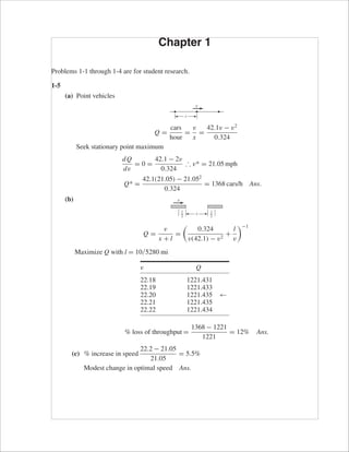
  • 1. Chapter 1 Problems 1-1 through 1-4 are for student research. 1-5 (a) Point vehicles Q = cars hour = v x = 42.1v − v2 0.324 Seek stationary point maximum dQ dv = 0 = 42.1 − 2v 0.324 ∴ v* = 21.05 mph Q* = 42.1(21.05) − 21.052 0.324 = 1368 cars/h Ans. (b) Q = v x + l = 0.324 v(42.1) − v2 + l v −1 Maximize Q with l = 10/5280 mi v Q 22.18 1221.431 22.19 1221.433 22.20 1221.435 ← 22.21 1221.435 22.22 1221.434 % loss of throughput = 1368 − 1221 1221 = 12% Ans. (c) % increase in speed 22.2 − 21.05 21.05 = 5.5% Modest change in optimal speed Ans. xl 2 l 2 v x v budy_sm_ch01.qxd 11/21/2006 15:23 Page 1
  • 2. 2 Solutions Manual • Instructor’s Solution Manual to Accompany Mechanical Engineering Design 1-6 This and the following problem may be the student’s first experience with a figure of merit. • Formulate fom to reflect larger figure of merit for larger merit. • Use a maximization optimization algorithm. When one gets into computer implementa- tion and answers are not known, minimizing instead of maximizing is the largest error one can make. FV = F1 sin θ − W = 0 FH = −F1 cos θ − F2 = 0 From which F1 = W/sin θ F2 = −W cos θ/sin θ fom = −$ = −¢γ (volume) . = −¢γ(l1 A1 + l2 A2) A1 = F1 S = W S sin θ , l2 = l1 cos θ A2 = F2 S = W cos θ S sin θ fom = −¢γ l2 cos θ W S sin θ + l2W cos θ S sin θ = −¢γ Wl2 S 1 + cos2 θ cos θ sin θ Set leading constant to unity θ◦ fom 0 −∞ 20 −5.86 30 −4.04 40 −3.22 45 −3.00 50 −2.87 54.736 −2.828 60 −2.886 Check second derivative to see if a maximum, minimum, or point of inflection has been found. Or, evaluate fom on either side of θ*. θ* = 54.736◦ Ans. fom* = −2.828 Alternative: d dθ 1 + cos2 θ cos θ sin θ = 0 And solve resulting tran- scendental for θ*. budy_sm_ch01.qxd 11/21/2006 15:23 Page 2
  • 3. Chapter 1 3 1-7 (a) x1 + x2 = X1 + e1 + X2 + e2 error = e = (x1 + x2) − (X1 + X2) = e1 + e2 Ans. (b) x1 − x2 = X1 + e1 − (X2 + e2) e = (x1 − x2) − (X1 − X2) = e1 − e2 Ans. (c) x1x2 = (X1 + e1)(X2 + e2) e = x1x2 − X1 X2 = X1e2 + X2e1 + e1e2 . = X1e2 + X2e1 = X1 X2 e1 X1 + e2 X2 Ans. (d) x1 x2 = X1 + e1 X2 + e2 = X1 X2 1 + e1/X1 1 + e2/X2 1 + e2 X2 −1 . = 1 − e2 X2 and 1 + e1 X1 1 − e2 X2 . = 1 + e1 X1 − e2 X2 e = x1 x2 − X1 X2 . = X1 X2 e1 X1 − e2 X2 Ans. 1-8 (a) x1 = √ 5 = 2.236 067 977 5 X1 = 2.23 3-correct digits x2 = √ 6 = 2.449 487 742 78 X2 = 2.44 3-correct digits x1 + x2 = √ 5 + √ 6 = 4.685 557 720 28 e1 = x1 − X1 = √ 5 − 2.23 = 0.006 067 977 5 e2 = x2 − X2 = √ 6 − 2.44 = 0.009 489 742 78 e = e1 + e2 = √ 5 − 2.23 + √ 6 − 2.44 = 0.015 557 720 28 Sum = x1 + x2 = X1 + X2 + e = 2.23 + 2.44 + 0.015 557 720 28 = 4.685 557 720 28 (Checks) Ans. (b) X1 = 2.24, X2 = 2.45 e1 = √ 5 − 2.24 = −0.003 932 022 50 e2 = √ 6 − 2.45 = −0.000 510 257 22 e = e1 + e2 = −0.004 442 279 72 Sum = X1 + X2 + e = 2.24 + 2.45 + (−0.004 442 279 72) = 4.685 557 720 28 Ans. budy_sm_ch01.qxd 11/21/2006 15:23 Page 3
  • 4. 4 Solutions Manual • Instructor’s Solution Manual to Accompany Mechanical Engineering Design 1-9 (a) σ = 20(6.89) = 137.8 MPa (b) F = 350(4.45) = 1558 N = 1.558 kN (c) M = 1200 lbf · in (0.113) = 135.6 N · m (d) A = 2.4(645) = 1548 mm2 (e) I = 17.4 in4 (2.54)4 = 724.2 cm4 (f) A = 3.6(1.610)2 = 9.332 km2 (g) E = 21(1000)(6.89) = 144.69(103 ) MPa = 144.7 GPa (h) v = 45 mi/h (1.61) = 72.45 km/h (i) V = 60 in3 (2.54)3 = 983.2 cm3 = 0.983 liter 1-10 (a) l = 1.5/0.305 = 4.918 ft = 59.02 in (b) σ = 600/6.89 = 86.96 kpsi (c) p = 160/6.89 = 23.22 psi (d) Z = 1.84(105 )/(25.4)3 = 11.23 in3 (e) w = 38.1/175 = 0.218 lbf/in (f) δ = 0.05/25.4 = 0.00197 in (g) v = 6.12/0.0051 = 1200 ft/min (h) = 0.0021 in/in (i) V = 30/(0.254)3 = 1831 in3 1-11 (a) σ = 200 15.3 = 13.1 MPa (b) σ = 42(103 ) 6(10−2)2 = 70(106 ) N/m2 = 70 MPa (c) y = 1200(800)3 (10−3 )3 3(207)109(64)103(10−3)4 = 1.546(10−2 ) m = 15.5 mm (d) θ = 1100(250)(10−3 ) 79.3(109)(π/32)(25)4(10−3)4 = 9.043(10−2 ) rad = 5.18◦ 1-12 (a) σ = 600 20(6) = 5 MPa (b) I = 1 12 8(24)3 = 9216 mm4 (c) I = π 64 324 (10−1 )4 = 5.147 cm4 (d) τ = 16(16) π(253)(10−3)3 = 5.215(106 ) N/m2 = 5.215 MPa budy_sm_ch01.qxd 11/21/2006 15:23 Page 4
  • 5. Chapter 1 5 1-13 (a) τ = 120(103 ) (π/4)(202) = 382 MPa (b) σ = 32(800)(800)(10−3 ) π(32)3(10−3)3 = 198.9(106 ) N/m2 = 198.9 MPa (c) Z = π 32(36) (364 − 264 ) = 3334 mm3 (d) k = (1.6)4 (10−3 )4 (79.3)(109 ) 8(19.2)3(10−3)3(32) = 286.8 N/m budy_sm_ch01.qxd 11/21/2006 15:23 Page 5
  • 6. FIRST PAGES 2-1 From Table A-20 Sut = 470 MPa (68 kpsi), Sy = 390 MPa (57 kpsi) Ans. 2-2 From Table A-20 Sut = 620 MPa (90 kpsi), Sy = 340 MPa (49.5 kpsi) Ans. 2-3 Comparison of yield strengths: Sut of G10500 HR is 620 470 = 1.32 times larger than SAE1020 CD Ans. Syt of SAE1020 CD is 390 340 = 1.15 times larger than G10500 HR Ans. From Table A-20, the ductilities (reduction in areas) show, SAE1020 CD is 40 35 = 1.14 times larger than G10500 Ans. The stiffness values of these materials are identical Ans. Table A-20 Table A-5 Sut Sy Ductility Stiffness MPa (kpsi) MPa (kpsi) R% GPa (Mpsi) SAE1020 CD 470(68) 390 (57) 40 207(30) UNS10500 HR 620(90) 340(495) 35 207(30) 2-4 From Table A-21 1040 Q&T ¯Sy = 593 (86) MPa (kpsi) at 205◦ C (400◦ F) Ans. 2-5 From Table A-21 1040 Q&T R = 65% at 650◦ C (1200◦ F) Ans. 2-6 Using Table A-5, the specific strengths are: UNS G10350 HR steel: Sy W = 39.5(103 ) 0.282 = 1.40(105 ) in Ans. 2024 T4 aluminum: Sy W = 43(103 ) 0.098 = 4.39(105 ) in Ans. Ti-6Al-4V titanium: Sy W = 140(103 ) 0.16 = 8.75(105 ) in Ans. ASTM 30 gray cast iron has no yield strength. Ans. Chapter 2 budynas_SM_ch02.qxd 11/22/2006 16:28 Page 6
  • 7. FIRST PAGES Chapter 2 7 2-7 The specific moduli are: UNS G10350 HR steel: E W = 30(106 ) 0.282 = 1.06(108 ) in Ans. 2024 T4 aluminum: E W = 10.3(106 ) 0.098 = 1.05(108 ) in Ans. Ti-6Al-4V titanium: E W = 16.5(106 ) 0.16 = 1.03(108 ) in Ans. Gray cast iron: E W = 14.5(106 ) 0.26 = 5.58(107 ) in Ans. 2-8 2G(1 + ν) = E ⇒ ν = E − 2G 2G From Table A-5 Steel: ν = 30 − 2(11.5) 2(11.5) = 0.304 Ans. Aluminum: ν = 10.4 − 2(3.90) 2(3.90) = 0.333 Ans. Beryllium copper: ν = 18 − 2(7) 2(7) = 0.286 Ans. Gray cast iron: ν = 14.5 − 2(6) 2(6) = 0.208 Ans. 2-9 0 10 0 0.002 0.1 0.004 0.2 0.006 0.3 0.008 0.4 0.010 0.5 0.012 0.6 0.014 0.7 0.016 0.8 (Lower curve) (Upper curve) 20 30 40 50 StressP͞A0kpsi Strain, ⑀ 60 70 80 E Y U Su ϭ 85.5 kpsi Ans. E ϭ 90͞0.003 ϭ 30 000 kpsi Ans. Sy ϭ 45.5 kpsi Ans. R ϭ (100) ϭ 45.8% Ans. A0 Ϫ AF A0 ϭ 0.1987 Ϫ 0.1077 0.1987 ⑀ ϭ ⌬l l0 ϭ l Ϫ l0 l0 l l0 ϭ Ϫ 1 A A0 ϭ Ϫ 1 budynas_SM_ch02.qxd 11/22/2006 16:28 Page 7
  • 8. FIRST PAGES 8 Solutions Manual • Instructor’s Solution Manual to Accompany Mechanical Engineering Design 2-10 To plot σtrue vs. ε, the following equations are applied to the data. A0 = π(0.503)2 4 = 0.1987 in2 Eq. (2-4) ε = ln l l0 for 0 ≤ L ≤ 0.0028 in ε = ln A0 A for L > 0.0028 in σtrue = P A The results are summarized in the table below and plotted on the next page. The last 5 points of data are used to plot log σ vs log ε The curve fit gives m = 0.2306 log σ0 = 5.1852 ⇒ σ0 = 153.2 kpsi Ans. For 20% cold work, Eq. (2-10) and Eq. (2-13) give, A = A0(1 − W) = 0.1987(1 − 0.2) = 0.1590 in2 ε = ln A0 A = ln 0.1987 0.1590 = 0.2231 Eq. (2-14): Sy = σ0εm = 153.2(0.2231)0.2306 = 108.4 kpsi Ans. Eq. (2-15), with Su = 85.5 kpsi from Prob. 2-9, Su = Su 1 − W = 85.5 1 − 0.2 = 106.9 kpsi Ans. P L A ε σtrue log ε log σtrue 0 0 0.198713 0 0 1000 0.0004 0.198713 0.0002 5032.388 −3.69901 3.701774 2000 0.0006 0.198713 0.0003 10064.78 −3.52294 4.002804 3000 0.0010 0.198713 0.0005 15097.17 −3.30114 4.178895 4000 0.0013 0.198713 0.00065 20129.55 −3.18723 4.303834 7000 0.0023 0.198713 0.001149 35226.72 −2.93955 4.546872 8400 0.0028 0.198713 0.001399 42272.06 −2.85418 4.626053 8800 0.0036 0.1984 0.001575 44354.84 −2.80261 4.646941 9200 0.0089 0.1978 0.004604 46511.63 −2.33685 4.667562 9100 0.1963 0.012216 46357.62 −1.91305 4.666121 13200 0.1924 0.032284 68607.07 −1.49101 4.836369 15200 0.1875 0.058082 81066.67 −1.23596 4.908842 17000 0.1563 0.240083 108765.2 −0.61964 5.03649 16400 0.1307 0.418956 125478.2 −0.37783 5.098568 14800 0.1077 0.612511 137418.8 −0.21289 5.138046 budynas_SM_ch02.qxd 11/22/2006 16:28 Page 8
  • 9. FIRST PAGES Chapter 2 9 2-11 Tangent modulus at σ = 0 is E0 = σ ε . = 5000 − 0 0.2(10−3) − 0 = 25(106 ) psi At σ = 20 kpsi E20 . = (26 − 19)(103 ) (1.5 − 1)(10−3) = 14.0(106 ) psi Ans. ε(10−3 ) σ (kpsi) 0 0 0.20 5 0.44 10 0.80 16 1.0 19 1.5 26 2.0 32 2.8 40 3.4 46 4.0 49 5.0 54 log ␧ log␴ y ϭ 0.2306x ϩ 5.1852 4.8 4.9 5 5.1 5.2 Ϫ1.6 Ϫ1.4 Ϫ1.2 Ϫ1 Ϫ0.8 Ϫ0.6 Ϫ0.4 Ϫ0.2 0 ␧true ␴true(psi) 0 20000 40000 60000 80000 100000 120000 140000 160000 0 0.1 0.2 0.3 0.4 0.5 0.6 0.7 ␧ (10Ϫ3 ) (Sy)0.001 ϭ˙ 35 kpsi Ans. ␴(kpsi) 0 10 20 30 40 50 60 0 1 2 3 4 5 budynas_SM_ch02.qxd 11/22/2006 16:28 Page 9
  • 10. FIRST PAGES 10 Solutions Manual • Instructor’s Solution Manual to Accompany Mechanical Engineering Design 2-12 Since |εo| = |εi | ln R + h R + N = ln R R + N = −ln R + N R R + h R + N = R + N R (R + N)2 = R(R + h) From which, N2 + 2RN − Rh = 0 The roots are: N = R −1 ± 1 + h R 1/2 The + sign being significant, N = R 1 + h R 1/2 − 1 Ans. Substitute for N in εo = ln R + h R + N Gives ε0 = ln      R + h R + R 1 + h R 1/2 − R      = ln 1 + h R 1/2 Ans. These constitute a useful pair of equations in cold-forming situations, allowing the surface strains to be found so that cold-working strength enhancement can be estimated. 2-13 From Table A-22 AISI 1212 Sy = 28.0 kpsi, σf = 106 kpsi, Sut = 61.5 kpsi σ0 = 110 kpsi, m = 0.24, εf = 0.85 From Eq. (2-12) εu = m = 0.24 Eq. (2-10) A0 Ai = 1 1 − W = 1 1 − 0.2 = 1.25 Eq. (2-13) εi = ln 1.25 = 0.2231 ⇒ εi < εu Eq. (2-14) Sy = σ0εm i = 110(0.2231)0.24 = 76.7 kpsi Ans. Eq. (2-15) Su = Su 1 − W = 61.5 1 − 0.2 = 76.9 kpsi Ans. 2-14 For HB = 250, Eq. (2-17) Su = 0.495 (250) = 124 kpsi = 3.41 (250) = 853 MPa Ans. budynas_SM_ch02.qxd 11/22/2006 16:28 Page 10
  • 11. FIRST PAGES Chapter 2 11 2-15 For the data given, HB = 2530 H2 B = 640 226 ¯HB = 2530 10 = 253 ˆσH B = 640 226 − (2530)2/10 9 = 3.887 Eq. (2-17) ¯Su = 0.495(253) = 125.2 kpsi Ans. ¯σsu = 0.495(3.887) = 1.92 kpsi Ans. 2-16 From Prob. 2-15, ¯HB = 253 and ˆσHB = 3.887 Eq. (2-18) ¯Su = 0.23(253) − 12.5 = 45.7 kpsi Ans. ˆσsu = 0.23(3.887) = 0.894 kpsi Ans. 2-17 (a) uR . = 45.52 2(30) = 34.5 in · lbf/in3 Ans. (b) P L A A0/A − 1 ε σ = P/A0 0 0 0 0 1000 0.0004 0.0002 5032.39 2000 0.0006 0.0003 10064.78 3000 0.0010 0.0005 15097.17 4000 0.0013 0.00065 20129.55 7000 0.0023 0.00115 35226.72 8400 0.0028 0.0014 42272.06 8800 0.0036 0.0018 44285.02 9200 0.0089 0.00445 46297.97 9100 0.1963 0.012291 0.012291 45794.73 13200 0.1924 0.032811 0.032811 66427.53 15200 0.1875 0.059802 0.059802 76492.30 17000 0.1563 0.271355 0.271355 85550.60 16400 0.1307 0.520373 0.520373 82531.17 14800 0.1077 0.845059 0.845059 74479.35 budynas_SM_ch02.qxd 11/22/2006 16:28 Page 11
  • 12. FIRST PAGES 12 Solutions Manual • Instructor’s Solution Manual to Accompany Mechanical Engineering Design uT . = 5 i=1 Ai = 1 2 (43 000)(0.001 5) + 45 000(0.004 45 − 0.001 5) + 1 2 (45 000 + 76 500)(0.059 8 − 0.004 45) + 81 000(0.4 − 0.059 8) + 80 000(0.845 − 0.4) . = 66.7(103 )in · lbf/in3 Ans. ␧ ␴ 0 20000 10000 30000 40000 50000 60000 70000 80000 90000 0 0.2 0.4 0.6 0.8 A3 A4 A5 Last 6 data points First 9 data points ␧ ␴ 0 A1 A215000 10000 5000 20000 25000 30000 35000 40000 45000 50000 0 0.0020.001 0.003 0.004 0.005 ␧ ␴ 0 20000 10000 30000 40000 50000 60000 70000 80000 90000 0 0.2 0.4 All data points 0.6 0.8 budynas_SM_ch02.qxd 11/22/2006 16:28 Page 12
  • 13. FIRST PAGES Chapter 2 13 2-18 m = Alρ For stiffness, k = AE/l, or, A = kl/E. Thus, m = kl2 ρ/E, and, M = E/ρ. Therefore, β = 1 From Fig. 2-16, ductile materials include Steel, Titanium, Molybdenum, Aluminum, and Composites. For strength, S = F/A, or, A = F/S. Thus, m = Fl ρ/S, and, M = S/ρ. From Fig. 2-19, lines parallel to S/ρ give for ductile materials, Steel, Nickel, Titanium, and composites. Common to both stiffness and strength are Steel, Titanium, Aluminum, and Composites. Ans. budynas_SM_ch02.qxd 11/22/2006 16:28 Page 13
  • 14. FIRST PAGES Chapter 3 3-1 1 RC RA RB RD C A B W D 1 23 RB RA W RB RC RA 2 1 W RA RBx RBx RBy RBy RB 2 1 1 Scale of corner magnified W A B (e) (f) (d) W A RA RB B 1 2 W A RA RB B 11 2 (a) (b) (c) budynas_SM_ch03.qxd 11/28/2006 21:21 Page 14
  • 15. FIRST PAGES Chapter 3 15 3-2 (a) RA = 2 sin 60 = 1.732 kN Ans. RB = 2 sin 30 = 1 kN Ans. (b) S = 0.6 m α = tan−1 0.6 0.4 + 0.6 = 30.96◦ RA sin 135 = 800 sin 30.96 ⇒ RA = 1100 N Ans. RO sin 14.04 = 800 sin 30.96 ⇒ RO = 377 N Ans. (c) RO = 1.2 tan 30 = 2.078 kN Ans. RA = 1.2 sin 30 = 2.4 kN Ans. (d) Step 1: Find RA and RE h = 4.5 tan 30 = 7.794 m ۗ+ MA = 0 9RE − 7.794(400 cos 30) − 4.5(400 sin 30) = 0 RE = 400 N Ans. Fx = 0 RAx + 400 cos 30 = 0 ⇒ RAx = −346.4 N Fy = 0 RAy + 400 − 400 sin 30 = 0 ⇒ RAy = −200 N RA = 346.42 + 2002 = 400 N Ans. D C h B y E xA 4.5 m 9 m 400 N 3 42 30° 60° RAy RA RAx RE 1.2 kN 60° RA RO 60°90° 30° 1.2 kN RARO 45Њ Ϫ 30.96Њ ϭ 14.04Њ 135° 30.96° 30.96° 800 N RA RO O 0.4 m 45° 800 N ␣ 0.6 m A s RA RO B 60° 90° 30° 2 kN RA RB 2 1 2 kN 60°30° RA RB budynas_SM_ch03.qxd 11/28/2006 21:21 Page 15
  • 16. FIRST PAGES 16 Solutions Manual • Instructor’s Solution Manual to Accompany Mechanical Engineering Design Step 2: Find components of RC on link 4 and RD ۗ+ MC = 0 400(4.5) − (7.794 − 1.9)RD = 0 ⇒ RD = 305.4 N Ans. Fx = 0 ⇒ (RCx)4 = 305.4 N Fy = 0 ⇒ (RCy)4 = −400 N Step 3: Find components of RC on link 2 Fx = 0 (RCx)2 + 305.4 − 346.4 = 0 ⇒ (RCx)2 = 41 N Fy = 0 (RCy)2 = 200 N 3-3 (a) ۗ+ M0 = 0 −18(60) + 14R2 + 8(30) − 4(40) = 0 R2 = 71.43 lbf Fy = 0: R1 − 40 + 30 + 71.43 − 60 = 0 R1 = −1.43 lbf M1 = −1.43(4) = −5.72 lbf · in M2 = −5.72 − 41.43(4) = −171.44 lbf · in M3 = −171.44 − 11.43(6) = −240 lbf · in M4 = −240 + 60(4) = 0 checks! 4" 4" 6" 4" Ϫ1.43 Ϫ41.43 Ϫ11.43 60 40 lbf 60 lbf 30 lbf x x x O A B C D y R1 R2 M1 M2 M3 M4 O V (lbf) M (lbf• in) O CC DB A B D E 305.4 N 346.4 N 305.4 N 41 N 400 N 200 N 400 N 200 N 400 N Pin C 30° 305.4 N 400 N 400 N200 N 41 N 305.4 N 200 N 346.4 N 305.4 N (RCx)2 (RCy)2 C B A 2 400 N 4 RD (RCx)4 (RCy)4 D C E Ans. budynas_SM_ch03.qxd 11/28/2006 21:21 Page 16
  • 17. FIRST PAGES Chapter 3 17 (b) Fy = 0 R0 = 2 + 4(0.150) = 2.6kN M0 = 0 M0 = 2000(0.2) + 4000(0.150)(0.425) = 655 N · m M1 = −655 + 2600(0.2) = −135 N · m M2 = −135 + 600(0.150) = −45 N · m M3 = −45 + 1 2 600(0.150) = 0 checks! (c) M0 = 0: 10R2 − 6(1000) = 0 ⇒ R2 = 600 lbf Fy = 0: R1 − 1000 + 600 = 0 ⇒ R1 = 400 lbf M1 = 400(6) = 2400 lbf · ft M2 = 2400 − 600(4) = 0 checks! (d) ۗ+ MC = 0 −10R1 + 2(2000) + 8(1000) = 0 R1 = 1200 lbf Fy = 0: 1200 − 1000 − 2000 + R2 = 0 R2 = 1800 lbf M1 = 1200(2) = 2400 lbf · ft M2 = 2400 + 200(6) = 3600 lbf · ft M3 = 3600 − 1800(2) = 0 checks! 2000 lbf1000 lbf R1 O O M1 M2 M3 R2 6 ft 2 ft2 ft A B C y M 1200 Ϫ1800 200 x x x 6 ft 4 ft A O O O B Ϫ600 M1 M2 V (lbf) 1000 lbfy R1 R2 400 M (lbf•ft) x x x V (kN) 150 mm200 mm 150 mm 2.6 Ϫ655 M (N•m) 0.6 M1 M2 M3 2 kN 4 kN/my A O O O O B C RO MO x x x budynas_SM_ch03.qxd 11/28/2006 21:21 Page 17
  • 18. FIRST PAGES 18 Solutions Manual • Instructor’s Solution Manual to Accompany Mechanical Engineering Design (e) ۗ+ MB = 0 −7R1 + 3(400) − 3(800) = 0 R1 = −171.4 lbf Fy = 0: −171.4 − 400 + R2 − 800 = 0 R2 = 1371.4 lbf M1 = −171.4(4) = −685.7 lbf · ft M2 = −685.7 − 571.4(3) = −2400 lbf · ft M3 = −2400 + 800(3) = 0 checks! (f) Break at A R1 = VA = 1 2 40(8) = 160 lbf ۗ + MD = 0 12(160) − 10R2 + 320(5) = 0 R2 = 352 lbf Fy = 0 −160 + 352 − 320 + R3 = 0 R3 = 128 lbf M1 = 1 2 160(4) = 320 lbf · in M2 = 320 − 1 2 160(4) = 0 checks! (hinge) M3 = 0 − 160(2) = −320 lbf · in M4 = −320 + 192(5) = 640 lbf · in M5 = 640 − 128(5) = 0 checks! 40 lbf/in V (lbf) O O 160 Ϫ160 Ϫ128 192 M 320 lbf 160 lbf 352 lbf 128 lbf M1 M2 M3 M4 M5 x x x 8" 5" 2" 5" 40 lbf/in 160 lbf O A y B D C A 320 lbf R2 R3 R1 VA A O O O C M V (lbf) 800 Ϫ171.4 Ϫ571.4 3 ft 3 ft4 ft 800 lbf400 lbf B y M1 M2 M3 R1 R2 x x x budynas_SM_ch03.qxd 11/28/2006 21:21 Page 18
  • 19. FIRST PAGES Chapter 3 19 3-4 (a) q = R1 x −1 − 40 x − 4 −1 + 30 x − 8 −1 + R2 x − 14 −1 − 60 x − 18 −1 V = R1 − 40 x − 4 0 + 30 x − 8 0 + R2 x − 14 0 − 60 x − 18 0 (1) M = R1x − 40 x − 4 1 + 30 x − 8 1 + R2 x − 14 1 − 60 x − 18 1 (2) for x = 18+ V = 0 and M = 0 Eqs. (1) and (2) give 0 = R1 − 40 + 30 + R2 − 60 ⇒ R1 + R2 = 70 (3) 0 = R1(18) − 40(14) + 30(10) + 4R2 ⇒ 9R1 + 2R2 = 130 (4) Solve (3) and (4) simultaneously to get R1 = −1.43 lbf, R2 = 71.43 lbf. Ans. From Eqs. (1) and (2), at x = 0+ , V = R1 = −1.43 lbf, M = 0 x = 4+ : V = −1.43 − 40 = −41.43, M = −1.43x x = 8+ : V = −1.43 − 40 + 30 = −11.43 M = −1.43(8) − 40(8 − 4)1 = −171.44 x = 14+ : V = −1.43 − 40 + 30 + 71.43 = 60 M = −1.43(14) − 40(14 − 4) + 30(14 − 8) = −240. x = 18+ : V = 0, M = 0 See curves of V and M in Prob. 3-3 solution. (b) q = R0 x −1 − M0 x −2 − 2000 x − 0.2 −1 − 4000 x − 0.35 0 + 4000 x − 0.5 0 V = R0 − M0 x −1 − 2000 x − 0.2 0 − 4000 x − 0.35 1 + 4000 x − 0.5 1 (1) M = R0x − M0 − 2000 x − 0.2 1 − 2000 x − 0.35 2 + 2000 x − 0.5 2 (2) at x = 0.5+ m, V = M = 0, Eqs. (1) and (2) give R0 − 2000 − 4000(0.5 − 0.35) = 0 ⇒ R1 = 2600 N = 2.6 kN Ans. R0(0.5) − M0 − 2000(0.5 − 0.2) − 2000(0.5 − 0.35)2 = 0 with R0 = 2600 N, M0 = 655 N · m Ans. With R0 and M0, Eqs. (1) and (2) give the same V and M curves as Prob. 3-3 (note for V, M0 x −1 has no physical meaning). (c) q = R1 x −1 − 1000 x − 6 −1 + R2 x − 10 −1 V = R1 − 1000 x − 6 0 + R2 x − 10 0 (1) M = R1x − 1000 x − 6 1 + R2 x − 10 1 (2) at x = 10+ ft, V = M = 0, Eqs. (1) and (2) give R1 − 1000 + R2 = 0 ⇒ R1 + R2 = 1000 10R1 − 1000(10 − 6) = 0 ⇒ R1 = 400 lbf, R2 = 1000 − 400 = 600 lbf 0 ≤ x ≤ 6: V = 400 lbf, M = 400x 6 ≤ x ≤ 10: V = 400 − 1000(x − 6)0 = 600 lbf M = 400x − 1000(x − 6) = 6000 − 600x See curves of Prob. 3-3 solution. (d) q = R1 x −1 − 1000 x − 2 −1 − 2000 x − 8 −1 + R2 x − 10 −1 V = R1 − 1000 x − 2 0 − 2000 x − 8 0 + R2 x − 10 0 (1) M = R1x − 1000 x − 2 1 − 2000 x − 8 1 + R2 x − 10 1 (2) budynas_SM_ch03.qxd 11/28/2006 21:21 Page 19
  • 20. FIRST PAGES 20 Solutions Manual • Instructor’s Solution Manual to Accompany Mechanical Engineering Design At x = 10+ , V = M = 0 from Eqs. (1) and (2) R1 − 1000 − 2000 + R2 = 0 ⇒ R1 + R2 = 3000 10R1 − 1000(10 − 2) − 2000(10 − 8) = 0 ⇒ R1 = 1200 lbf, R2 = 3000 − 1200 = 1800 lbf 0 ≤ x ≤ 2: V = 1200 lbf, M = 1200x lbf · ft 2 ≤ x ≤ 8: V = 1200 − 1000 = 200 lbf M = 1200x − 1000(x − 2) = 200x + 2000 lbf · ft 8 ≤ x ≤ 10: V = 1200 − 1000 − 2000 = −1800 lbf M = 1200x − 1000(x − 2) − 2000(x − 8) = −1800x + 18 000 lbf · ft Plots are the same as in Prob. 3-3. (e) q = R1 x −1 − 400 x − 4 −1 + R2 x − 7 −1 − 800 x − 10 −1 V = R1 − 400 x − 4 0 + R2 x − 7 0 − 800 x − 10 0 (1) M = R1x − 400 x − 4 1 + R2 x − 7 1 − 800 x − 10 1 (2) at x = 10+ , V = M = 0 R1 − 400 + R2 − 800 = 0 ⇒ R1 + R2 = 1200 (3) 10R1 − 400(6) + R2(3) = 0 ⇒ 10R1 + 3R2 = 2400 (4) Solve Eqs. (3) and (4) simultaneously: R1 = −171.4 lbf, R2 = 1371.4 lbf 0 ≤ x ≤ 4: V = −171.4 lbf, M = −171.4x lbf · ft 4 ≤ x ≤ 7: V = −171.4 − 400 = −571.4 lbf M = −171.4x − 400(x − 4) lbf · ft = −571.4x + 1600 7 ≤ x ≤ 10: V = −171.4 − 400 + 1371.4 = 800 lbf M = −171.4x − 400(x − 4) + 1371.4(x − 7) = 800x − 8000 lbf · ft Plots are the same as in Prob. 3-3. (f) q = R1 x −1 − 40 x 0 + 40 x − 8 0 + R2 x − 10 −1 − 320 x − 15 −1 + R3 x − 20 V = R1 − 40x + 40 x − 8 1 + R2 x − 10 0 − 320 x − 15 0 + R3 x − 20 0 (1) M = R1x − 20x2 + 20 x − 8 2 + R2 x − 10 1 − 320 x − 15 1 + R3 x − 20 1 (2) M = 0 at x = 8 in ∴ 8R1 − 20(8)2 = 0 ⇒ R1 = 160 lbf at x = 20+ , V and M = 0 160 − 40(20) + 40(12) + R2 − 320 + R3 = 0 ⇒ R2 + R3 = 480 160(20) − 20(20)2 + 20(12)2 + 10R2 − 320(5) = 0 ⇒ R2 = 352 lbf R3 = 480 − 352 = 128 lbf 0 ≤ x ≤ 8: V = 160 − 40x lbf, M = 160x − 20x2 lbf · in 8 ≤ x ≤ 10: V = 160 − 40x + 40(x − 8) = −160 lbf, M = 160x − 20x2 + 20(x − 8)2 = 1280 − 160x lbf · in 10 ≤ x ≤ 15: V = 160 − 40x + 40(x − 8) + 352 = 192 lbf M = 160x − 20x2 + 20(x − 8) + 352(x − 10) = 192x − 2240 budynas_SM_ch03.qxd 11/28/2006 21:21 Page 20
  • 21. FIRST PAGES Chapter 3 21 15 ≤ x ≤ 20: V = 160 − 40x + 40(x − 8) + 352 − 320 = −128 lbf M = 160x − 20x2 − 20(x − 8) + 352(x − 10) − 320(x − 15) = −128x + 2560 Plots of V and M are the same as in Prob. 3-3. 3-5 Solution depends upon the beam selected. 3-6 (a) Moment at center, xc = (l − 2a)/2 Mc = w 2 l 2 (l − 2a) − l 2 2 = wl 2 l 4 − a At reaction, |Mr | = wa2 /2 a = 2.25, l = 10 in, w = 100 lbf/in Mc = 100(10) 2 10 4 − 2.25 = 125 lbf · in Mr = 100(2.252 ) 2 = 253.1 lbf · in Ans. (b) Minimum occurs when Mc = |Mr | wl 2 l 4 − a = wa2 2 ⇒ a2 + al − 0.25l2 = 0 Taking the positive root a = 1 2 −l + l2 + 4(0.25l2) = l 2 √ 2 − 1 = 0.2071l Ans. for l = 10 in and w = 100 lbf, Mmin = (100/2)[(0.2071)(10)]2 = 214 lbf · in 3-7 For the ith wire from bottom, from summing forces vertically (a) Ti = (i + 1)W From summing moments about point a, Ma = W(l − xi ) − iW xi = 0 Giving, xi = l i + 1 W iW Ti xi a budynas_SM_ch03.qxd 11/28/2006 21:21 Page 21
  • 22. FIRST PAGES 22 Solutions Manual • Instructor’s Solution Manual to Accompany Mechanical Engineering Design So W = l 1 + 1 = l 2 x = l 2 + 1 = l 3 y = l 3 + 1 = l 4 z = l 4 + 1 = l 5 (b) With straight rigid wires, the mobile is not stable. Any perturbation can lead to all wires becoming collinear. Consider a wire of length l bent at its string support: Ma = 0 Ma = iWl i + 1 cos α − ilW i + 1 cos β = 0 iWl i + 1 (cos α − cos β) = 0 Moment vanishes when α = β for any wire. Consider a ccw rotation angle β, which makes α → α + β and β → α − β Ma = iWl i + 1 [cos(α + β) − cos(α − β)] = 2iWl i + 1 sin α sin β . = 2iWlβ i + 1 sin α There exists a correcting moment of opposite sense to arbitrary rotation β. An equation for an upward bend can be found by changing the sign of W. The moment will no longer be correcting. A curved, convex-upward bend of wire will produce stable equilibrium too, but the equation would change somewhat. 3-8 (a) C = 12 + 6 2 = 9 CD = 12 − 6 2 = 3 R = 32 + 42 = 5 σ1 = 5 + 9 = 14 σ2 = 9 − 5 = 4 2␾s (12, 4cw ) C R D ␶2 ␶1 ␴1 ␴␴2 2␾p (6, 4ccw ) y x ␶cw ␶ccw W iW il i ϩ 1 Ti ␤␣ l i ϩ 1 budynas_SM_ch03.qxd 11/28/2006 21:21 Page 22
  • 23. FIRST PAGES Chapter 3 23 φp = 1 2 tan−1 4 3 = 26.6◦ cw τ1 = R = 5, φs = 45◦ − 26.6◦ = 18.4◦ ccw (b) C = 9 + 16 2 = 12.5 CD = 16 − 9 2 = 3.5 R = 52 + 3.52 = 6.10 σ1 = 6.1 + 12.5 = 18.6 φp = 1 2 tan−1 5 3.5 = 27.5◦ ccw σ2 = 12.5 − 6.1 = 6.4 τ1 = R = 6.10, φs = 45◦ − 27.5◦ = 17.5◦ cw (c) C = 24 + 10 2 = 17 CD = 24 − 10 2 = 7 R = 72 + 62 = 9.22 σ1 = 17 + 9.22 = 26.22 σ2 = 17 − 9.22 = 7.78 2␾s (24, 6cw ) C R D ␶2 ␶1 ␴1␴2 2␾p (10, 6ccw ) y x ␴ ␶cw ␶ccw x 12.5 12.5 6.10 17.5Њ x 6.4 18.6 27.5Њ 2␾s (16, 5ccw ) C R D ␶2 ␶1 ␴1␴2 2␾p (9, 5cw ) y x ␴ ␶cw ␶ccw 9 5 9 9 9 18.4Њ x x 4 14 26.6Њ budynas_SM_ch03.qxd 11/28/2006 21:21 Page 23
  • 24. FIRST PAGES 24 Solutions Manual • Instructor’s Solution Manual to Accompany Mechanical Engineering Design φp = 1 2 90 + tan−1 7 6 = 69.7◦ ccw τ1 = R = 9.22, φs = 69.7◦ − 45◦ = 24.7◦ ccw (d) C = 9 + 19 2 = 14 CD = 19 − 9 2 = 5 R = 52 + 82 = 9.434 σ1 = 14 + 9.43 = 23.43 σ2 = 14 − 9.43 = 4.57 φp = 1 2 90 + tan−1 5 8 = 61.0◦ cw τ1 = R = 9.434, φs = 61◦ − 45◦ = 16◦ cw x 14 14 9.434 16Њ x 23.43 4.57 61Њ 2␾s (9, 8cw ) C R D ␶2 ␶1 ␴1␴2 2␾p (19, 8ccw ) y x ␴ ␶cw ␶ccw x 17 17 9.22 24.7Њ x 26.22 7.78 69.7Њ budynas_SM_ch03.qxd 11/28/2006 21:21 Page 24
  • 25. FIRST PAGES Chapter 3 25 3-9 (a) C = 12 − 4 2 = 4 CD = 12 + 4 2 = 8 R = 82 + 72 = 10.63 σ1 = 4 + 10.63 = 14.63 σ2 = 4 − 10.63 = −6.63 φp = 1 2 90 + tan−1 8 7 = 69.4◦ ccw τ1 = R = 10.63, φs = 69.4◦ − 45◦ = 24.4◦ ccw (b) C = 6 − 5 2 = 0.5 CD = 6 + 5 2 = 5.5 R = 5.52 + 82 = 9.71 σ1 = 0.5 + 9.71 = 10.21 σ2 = 0.5 − 9.71 = −9.21 φp = 1 2 tan−1 8 5.5 = 27.75◦ ccw x 10.21 9.21 27.75Њ 2␾s (Ϫ5, 8cw ) C R D ␶2 ␶1 ␴1 ␴ ␴2 2␾p (6, 8ccw ) y x ␶cw ␶ccw x 4 4 10.63 24.4Њ x 14.63 6.63 69.4Њ 2␾s (12, 7cw ) C R D ␶2 ␶1 ␴1 ␴␴2 2␾p (Ϫ4, 7ccw ) y x ␶cw ␶ccw budynas_SM_ch03.qxd 11/28/2006 21:22 Page 25
  • 26. FIRST PAGES 26 Solutions Manual • Instructor’s Solution Manual to Accompany Mechanical Engineering Design τ1 = R = 9.71, φs = 45◦ − 27.75◦ = 17.25◦ cw (c) C = −8 + 7 2 = −0.5 CD = 8 + 7 2 = 7.5 R = 7.52 + 62 = 9.60 σ1 = 9.60 − 0.5 = 9.10 σ2 = −0.5 − 9.6 = −10.1 φp = 1 2 90 + tan−1 7.5 6 = 70.67◦ cw τ1 = R = 9.60, φs = 70.67◦ − 45◦ = 25.67◦ cw (d) C = 9 − 6 2 = 1.5 CD = 9 + 6 2 = 7.5 R = 7.52 + 32 = 8.078 σ1 = 1.5 + 8.078 = 9.58 σ2 = 1.5 − 8.078 = −6.58 2␾s (9, 3cw ) CR D ␶2 ␶1 ␴1␴2 2␾p (Ϫ6, 3ccw ) y x ␴ ␶cw ␶ccw x 0.5 0.5 9.60 25.67Њ x 10.1 9.1 70.67Њ 2␾s (Ϫ8, 6cw ) C R D ␶2 ␶1 ␴1␴2 2␾p (7, 6ccw ) x y ␴ ␶cw ␶ccw x 0.5 0.5 9.71 17.25Њ budynas_SM_ch03.qxd 11/28/2006 21:22 Page 26
  • 27. FIRST PAGES Chapter 3 27 φp = 1 2 tan−1 3 7.5 = 10.9◦ cw τ1 = R = 8.078, φs = 45◦ − 10.9◦ = 34.1◦ ccw 3-10 (a) C = 20 − 10 2 = 5 CD = 20 + 10 2 = 15 R = 152 + 82 = 17 σ1 = 5 + 17 = 22 σ2 = 5 − 17 = −12 φp = 1 2 tan−1 8 15 = 14.04◦ cw τ1 = R = 17, φs = 45◦ − 14.04◦ = 30.96◦ ccw 5 17 5 30.96Њ x 12 22 14.04Њ x 2␾s (20, 8cw ) C R D ␶2 ␶1 ␴1␴2 2␾p (Ϫ10, 8ccw ) y x ␴ ␶cw ␶ccw x 1.5 8.08 1.5 34.1Њ x 6.58 9.58 10.9Њ budynas_SM_ch03.qxd 11/28/2006 21:22 Page 27
  • 28. FIRST PAGES 28 Solutions Manual • Instructor’s Solution Manual to Accompany Mechanical Engineering Design (b) C = 30 − 10 2 = 10 CD = 30 + 10 2 = 20 R = 202 + 102 = 22.36 σ1 = 10 + 22.36 = 32.36 σ2 = 10 − 22.36 = −12.36 φp = 1 2 tan−1 10 20 = 13.28◦ ccw τ1 = R = 22.36, φs = 45◦ − 13.28◦ = 31.72◦ cw (c) C = −10 + 18 2 = 4 CD = 10 + 18 2 = 14 R = 142 + 92 = 16.64 σ1 = 4 + 16.64 = 20.64 σ2 = 4 − 16.64 = −12.64 φp = 1 2 90 + tan−1 14 9 = 73.63◦ cw τ1 = R = 16.64, φs = 73.63◦ − 45◦ = 28.63◦ cw 4 x 16.64 4 28.63Њ 12.64 20.64 73.63Њ x 2␾s(Ϫ10, 9cw ) C R D ␶2 ␶1 ␴1␴2 2␾p (18, 9ccw ) y x ␴ ␶cw ␶ccw 10 10 22.36 31.72Њ x 12.36 32.36 x 13.28Њ 2␾s (Ϫ10, 10cw ) C R D ␶2 ␶1 ␴1 ␴ ␴2 2␾p (30, 10ccw ) y x ␶cw ␶ccw budynas_SM_ch03.qxd 11/28/2006 21:22 Page 28
  • 29. FIRST PAGES Chapter 3 29 (d) C = −12 + 22 2 = 5 CD = 12 + 22 2 = 17 R = 172 + 122 = 20.81 σ1 = 5 + 20.81 = 25.81 σ2 = 5 − 20.81 = −15.81 φp = 1 2 90 + tan−1 17 12 = 72.39◦ cw τ1 = R = 20.81, φs = 72.39◦ − 45◦ = 27.39◦ cw 3-11 (a) (b) C = 0 + 10 2 = 5 CD = 10 − 0 2 = 5 R = 52 + 42 = 6.40 σ1 = 5 + 6.40 = 11.40 σ2 = 0, σ3 = 5 − 6.40 = −1.40 τ1/3 = R = 6.40, τ1/2 = 11.40 2 = 5.70, τ2/3 = 1.40 2 = 0.70 ␴1␴2 ␴ ␴3 D x y ␶ C R (0, 4cw ) (10, 4ccw ) ␶2/3 ␶1/2 ␶1/3 ␴x ϭ ␴1 ␴ ␴3 ϭ ␴y ␶ ␴2 ϭ 0 Ϫ4 10y x ␶2/3 ϭ 2 ␶1/2 ϭ 5 ␶1/3 ϭ ϭ 7 14 2 5 20.81 5 27.39Њ x 15.81 25.81 72.39Њ x 2␾s(Ϫ12, 12cw ) C R D ␶2 ␶1 ␴1␴2 2␾p (22, 12ccw ) y x ␴ ␶cw ␶ccw budynas_SM_ch03.qxd 11/28/2006 21:22 Page 29
  • 30. FIRST PAGES 30 Solutions Manual • Instructor’s Solution Manual to Accompany Mechanical Engineering Design (c) C = −2 − 8 2 = −5 CD = 8 − 2 2 = 3 R = 32 + 42 = 5 σ1 = −5 + 5 = 0, σ2 = 0 σ3 = −5 − 5 = −10 τ1/3 = 10 2 = 5, τ1/2 = 0, τ2/3 = 5 (d) C = 10 − 30 2 = −10 CD = 10 + 30 2 = 20 R = 202 + 102 = 22.36 σ1 = −10 + 22.36 = 12.36 σ2 = 0 σ3 = −10 − 22.36 = −32.36 τ1/3 = 22.36, τ1/2 = 12.36 2 = 6.18, τ2/3 = 32.36 2 = 16.18 3-12 (a) C = −80 − 30 2 = −55 CD = 80 − 30 2 = 25 R = 252 + 202 = 32.02 σ1 = 0 σ2 = −55 + 32.02 = −22.98 = −23.0 σ3 = −55 − 32.0 = −87.0 τ1/2 = 23 2 = 11.5, τ2/3 = 32.0, τ1/3 = 87 2 = 43.5 ␴1 (Ϫ80, 20cw ) (Ϫ30, 20ccw ) C D R ␶2/3 ␶1/2 ␶1/3 ␴2␴3 x y ␶ ␴ ␴1 (Ϫ30, 10cw ) (10, 10ccw ) C D R ␶2/3 ␶1/2 ␶␶1/3 ␴2␴3 ␴ y x ␴1␴2 ␴ ␶ ␴3 (Ϫ2, 4cw ) Point is a circle 2 circles C D y x (Ϫ8, 4ccw ) budynas_SM_ch03.qxd 11/28/2006 21:22 Page 30
  • 31. FIRST PAGES Chapter 3 31 (b) C = 30 − 60 2 = −15 CD = 60 + 30 2 = 45 R = 452 + 302 = 54.1 σ1 = −15 + 54.1 = 39.1 σ2 = 0 σ3 = −15 − 54.1 = −69.1 τ1/3 = 39.1 + 69.1 2 = 54.1, τ1/2 = 39.1 2 = 19.6, τ2/3 = 69.1 2 = 34.6 (c) C = 40 + 0 2 = 20 CD = 40 − 0 2 = 20 R = 202 + 202 = 28.3 σ1 = 20 + 28.3 = 48.3 σ2 = 20 − 28.3 = −8.3 σ3 = σz = −30 τ1/3 = 48.3 + 30 2 = 39.1, τ1/2 = 28.3, τ2/3 = 30 − 8.3 2 = 10.9 (d) C = 50 2 = 25 CD = 50 2 = 25 R = 252 + 302 = 39.1 σ1 = 25 + 39.1 = 64.1 σ2 = 25 − 39.1 = −14.1 σ3 = σz = −20 τ1/3 = 64.1 + 20 2 = 42.1, τ1/2 = 39.1, τ2/3 = 20 − 14.1 2 = 2.95 ␴1 (50, 30cw ) (0, 30ccw ) C D ␶2/3 ␶1/2 ␶1/3 ␴2␴3 x y ␴ ␶ ␴1 (0, 20cw ) (40, 20ccw ) C D R ␶2/3 ␶1/2 ␶1/3 ␴2␴3 y x ␴ ␶ ␴1 ␴ ␶ (Ϫ60, 30ccw ) (30, 30cw ) C D R ␶2/3 ␶1/2 ␶1/3 ␴2␴3 x y budynas_SM_ch03.qxd 11/28/2006 21:22 Page 31
  • 32. FIRST PAGES 32 Solutions Manual • Instructor’s Solution Manual to Accompany Mechanical Engineering Design 3-13 σ = F A = 2000 (π/4)(0.52) = 10 190 psi = 10.19 kpsi Ans. δ = FL AE = σ L E = 10 190 72 30(106) = 0.024 46 in Ans. 1 = δ L = 0.024 46 72 = 340(10−6 ) = 340µ Ans. From Table A-5, ν = 0.292 2 = −ν 1 = −0.292(340) = −99.3µ Ans. d = 2d = −99.3(10−6 )(0.5) = −49.6(10−6 ) in Ans. 3-14 From Table A-5, E = 71.7 GPa δ = σ L E = 135(106 ) 3 71.7(109) = 5.65(10−3 ) m = 5.65 mm Ans. 3-15 With σz = 0, solve the first two equations of Eq. (3-19) simultaneously. Place E on the left- hand side of both equations, and using Cramer’s rule, σx = E x −ν E y 1 1 −ν −ν 1 = E x + νE y 1 − ν2 = E( x + ν y) 1 − ν2 Likewise, σy = E( y + ν x) 1 − ν2 From Table A-5, E = 207 GPa and ν = 0.292. Thus, σx = E( x + ν y) 1 − ν2 = 207(109 )[0.0021 + 0.292(−0.000 67)] 1 − 0.2922 (10−6 ) = 431 MPa Ans. σy = 207(109 )[−0.000 67 + 0.292(0.0021)] 1 − 0.2922 (10−6 ) = −12.9 MPa Ans. 3-16 The engineer has assumed the stress to be uniform. That is, Ft = −F cos θ + τ A = 0 ⇒ τ = F A cos θ When failure occurs in shear Ssu = F A cos θ ␶ ␴ t ␪ F budynas_SM_ch03.qxd 11/28/2006 21:22 Page 32
  • 33. FIRST PAGES Chapter 3 33 The uniform stress assumption is common practice but is not exact. If interested in the details, see p. 570 of 6th edition. 3-17 From Eq. (3-15) σ3 − (−2 + 6 − 4)σ2 + [−2(6) + (−2)(−4) + 6(−4) − 32 − 22 − (−5)2 ]σ − [−2(6)(−4) + 2(3)(2)(−5) − (−2)(2)2 − 6(−5)2 − (−4)(3)2 ] = 0 σ3 − 66σ + 118 = 0 Roots are: 7.012, 1.89, −8.903 kpsi Ans. τ1/2 = 7.012 − 1.89 2 = 2.56 kpsi τ2/3 = 8.903 + 1.89 2 = 5.40 kpsi τmax = τ1/3 = 8.903 + 7.012 2 = 7.96 kpsi Ans. Note: For Probs. 3-17 to 3-19, one can also find the eigenvalues of the matrix [σ] = σx τxy τzx τxy σy τyz τzx τyz σz for the principal stresses 3-18 From Eq. (3-15) σ3 − (10 + 0 + 10)σ2 + 10(0) + 10(10) + 0(10) − 202 − −10 √ 2 2 − 02 σ − 10(0)(10) + 2(20) −10 √ 2 (0) − 10 −10 √ 2 2 − 0(0)2 − 10(20)2 = 0 σ3 − 20σ2 − 500σ + 6000 = 0 Roots are: 30, 10, −20 MPa Ans. τ1/2 = 30 − 10 2 = 10 MPa τ2/3 = 10 + 20 2 = 15 MPa τmax = τ1/3 = 30 + 20 2 = 25 MPa Ans. 3010Ϫ20 ␶2/3 ␶1/2 ␶1/3 ␴ (MPa) ␶ (MPa) 7.0121.89 Ϫ8.903 ␶2/3 ␶1/2 ␶1/3 ␶ (kpsi) ␴ (kpsi) budynas_SM_ch03.qxd 11/28/2006 21:22 Page 33
  • 34. FIRST PAGES 34 Solutions Manual • Instructor’s Solution Manual to Accompany Mechanical Engineering Design 3-19 From Eq. (3-15) σ3 − (1 + 4 + 4)σ2 + [1(4) + 1(4) + 4(4) − 22 − (−4)2 − (−2)2 ]σ −[1(4)(4) + 2(2)(−4)(−2) − 1(−4)2 − 4(−2)2 − 4(2)2 ] = 0 σ3 − 9σ2 = 0 Roots are: 9, 0, 0 kpsi τ2/3 = 0, τ1/2 = τ1/3 = τmax = 9 2 = 4.5 kpsi Ans. 3-20 (a) R1 = c l F Mmax = R1a = ac l F σ = 6M bh2 = 6 bh2 ac l F ⇒ F = σbh2 l 6ac Ans. (b) Fm F = (σm/σ)(bm/b) (hm/h)2 (lm/l) (am/a) (cm/c) = 1(s)(s)2 (s) (s)(s) = s2 Ans. For equal stress, the model load varies by the square of the scale factor. 3-21 R1 = wl 2 , Mmax|x=l/2 = w 2 l 2 l − l 2 = wl2 8 σ = 6M bh2 = 6 bh2 wl2 8 = 3Wl 4bh2 ⇒ W = 4 3 σbh2 l Ans. Wm W = (σm/σ)(bm/b) (hm/h)2 lm/l = 1(s)(s)2 s = s2 Ans. wmlm wl = s2 ⇒ wm w = s2 s = s Ans. For equal stress, the model load w varies linearily with the scale factor. ␶2/3 ␶(kpsi) ␴(kpsi) ␶1/2 ϭ ␶1/3 O 0 9 budynas_SM_ch03.qxd 11/28/2006 21:22 Page 34
  • 35. FIRST PAGES Chapter 3 35 3-22 (a) Can solve by iteration or derive equations for the general case. Find maximum moment under wheel W3 WT = W at centroid of W’s RA = l − x3 − d3 l WT Under wheel 3 M3 = RAx3 − W1a13 − W2a23 = (l − x3 − d3) l WT x3 − W1a13 − W2a23 For maximum, dM3 dx3 = 0 = (l − d3 − 2x3) WT l ⇒ x3 = l − d3 2 substitute into M, ⇒ M3 = (l − d3)2 4l WT − W1a13 − W2a23 This means the midpoint of d3 intersects the midpoint of the beam For wheel i xi = l − di 2 , Mi = (l − di )2 4l WT − i−1 j=1 Wjaji Note for wheel 1: Wjaji = 0 WT = 104.4, W1 = W2 = W3 = W4 = 104.4 4 = 26.1 kip Wheel 1: d1 = 476 2 = 238 in, M1 = (1200 − 238)2 4(1200) (104.4) = 20 128 kip · in Wheel 2: d2 = 238 − 84 = 154 in M2 = (1200 − 154)2 4(1200) (104.4) − 26.1(84) = 21 605 kip · in = Mmax Check if all of the wheels are on the rail (b) xmax = 600 − 77 = 523 in (c) See above sketch. (d) inner axles 600" 600" 84" 77" 84" 315" xmax RA W1 A B W3 . . . . . .W2 WT d3 Wn RB a23 a13 x3 l budynas_SM_ch03.qxd 11/28/2006 21:22 Page 35
  • 36. FIRST PAGES 36 Solutions Manual • Instructor’s Solution Manual to Accompany Mechanical Engineering Design 3-23 (a) Aa = Ab = 0.25(1.5) = 0.375 in2 A = 3(0.375) = 1.125 in2 ¯y = 2(0.375)(0.75) + 0.375(0.5) 1.125 = 0.667 in Ia = 0.25(1.5)3 12 = 0.0703 in4 Ib = 1.5(0.25)3 12 = 0.001 95 in4 I1 = 2[0.0703 + 0.375(0.083)2 ] + [0.001 95 + 0.375(0.167)2 ] = 0.158 in4 Ans. σA = 10 000(0.667) 0.158 = 42(10)3 psi Ans. σB = 10 000(0.667 − 0.375) 0.158 = 18.5(10)3 psi Ans. σC = 10 000(0.167 − 0.125) 0.158 = 2.7(10)3 psi Ans. σD = − 10 000(0.833) 0.158 = −52.7(10)3 psi Ans. (b) Here we treat the hole as a negative area. Aa = 1.732 in2 Ab = 1.134 0.982 2 = 0.557 in2 D C B A y 11 a b A Ga Gb0.327" 0.25" c1 ϭ 1.155" c2 ϭ 0.577" 2" 1.732" 0.577" 0.982" 0.577" 1.134" 1 2 1 " 1 4 " 3 8 " 1 4 " 1 4 " D C 1 1 Ga Gb c1 ϭ 0.833" 0.167" 0.083" 0.5" 0.75" 1.5" y ϭ c2 ϭ 0.667" B aa b A budynas_SM_ch03.qxd 11/28/2006 21:22 Page 36
  • 37. FIRST PAGES Chapter 3 37 A = 1.732 − 0.557 = 1.175 in2 ¯y = 1.732(0.577) − 0.557(0.577) 1.175 = 0.577 in Ans. Ia = bh3 36 = 2(1.732)3 36 = 0.289 in4 Ib = 1.134(0.982)3 36 = 0.0298 in4 I1 = Ia − Ib = 0.289 − 0.0298 = 0.259 in4 Ans. because the centroids are coincident. σA = 10 000(0.577) 0.259 = 22.3(10)3 psi Ans. σB = 10 000(0.327) 0.259 = 12.6(10)3 psi Ans. σC = − 10 000(0.982 − 0.327) 0.259 = −25.3(10)3 psi Ans. σD = − 10 000(1.155) 0.259 = −44.6(10)3 psi Ans. (c) Use two negative areas. Aa = 1 in2 , Ab = 9 in2 , Ac = 16 in2 , A = 16 − 9 − 1 = 6 in2 ; ¯ya = 0.25 in, ¯yb = 2.0 in, ¯yc = 2 in ¯y = 16(2) − 9(2) − 1(0.25) 6 = 2.292 in Ans. c1 = 4 − 2.292 = 1.708 in Ia = 2(0.5)3 12 = 0.020 83 in4 Ib = 3(3)3 12 = 6.75 in4 Ic = 4(4)3 12 = 21.333 in4 D C c a B b A Ga Gb Gc c1 ϭ 1.708" c2 ϭ 2.292" 2" 1.5" 0.25" 11 budynas_SM_ch03.qxd 11/28/2006 21:22 Page 37
  • 38. FIRST PAGES 38 Solutions Manual • Instructor’s Solution Manual to Accompany Mechanical Engineering Design I1 = [21.333 + 16(0.292)2 ] − [6.75 + 9(0.292)2 ] − [0.020 83 + 1(2.292 − 0.25)2 ] = 10.99 in4 Ans. σA = 10 000(2.292) 10.99 = 2086 psi Ans. σB = 10 000(2.292 − 0.5) 10.99 = 1631 psi Ans. σC = − 10 000(1.708 − 0.5) 10.99 = −1099 psi Ans. σD = − 10 000(1.708) 10.99 = −1554 psi Ans. (d) Use a as a negative area. Aa = 6.928 in2 , Ab = 16 in2 , A = 9.072 in2 ; ¯ya = 1.155 in, ¯yb = 2 in ¯y = 2(16) − 1.155(6.928) 9.072 = 2.645 in Ans. c1 = 4 − 2.645 = 1.355 in Ia = bh3 36 = 4(3.464)3 36 = 4.618 in4 Ib = 4(4)3 12 = 21.33 in4 I1 = [21.33 + 16(0.645)2 ] − [4.618 + 6.928(1.490)2 ] = 7.99 in4 Ans. σA = 10 000(2.645) 7.99 = 3310 psi Ans. σB = − 10 000(3.464 − 2.645) 7.99 = −1025 psi Ans. σC = − 10 000(1.355) 7.99 = −1696 psi Ans. 3.464" 11 Ga B b a C A c1 ϭ 1.355" c2 ϭ 2.645" 1.490" 1.155" budynas_SM_ch03.qxd 11/28/2006 21:22 Page 38
  • 39. FIRST PAGES Chapter 3 39 (e) Aa = 6(1.25) = 7.5 in2 Ab = 3(1.5) = 4.5 in2 A = Ac + Ab = 12 in2 ¯y = 3.625(7.5) + 1.5(4.5) 12 = 2.828 in Ans. I = 1 12 (6)(1.25)3 + 7.5(3.625 − 2.828)2 + 1 12 (1.5)(3)3 + 4.5(2.828 − 1.5)2 = 17.05 in4 Ans. σA = 10 000(2.828) 17.05 = 1659 psi Ans. σB = − 10 000(3 − 2.828) 17.05 = −101 psi Ans. σC = − 10 000(1.422) 17.05 = −834 psi Ans. (f) Let a = total area A = 1.5(3) − 1(1.25) = 3.25 in2 I = Ia − 2Ib = 1 12 (1.5)(3)3 − 1 12 (1.25)(1)3 = 3.271 in4 Ans. σA = 10 000(1.5) 3.271 = 4586 psi, σD = −4586 psi Ans. σB = 10 000(0.5) 3.271 = 1529 psi, σC = −1529 psi 3-24 (a) The moment is maximum and constant between A and B M = −50(20) = −1000 lbf · in, I = 1 12 (0.5)(2)3 = 0.3333 in4 ρ = E I M = 1.6(106 )(0.3333) 1000 = 533.3 in (x, y) = (30, −533.3) in Ans. (b) The moment is maximum and constant between A and B M = 50(5) = 250 lbf · in, I = 0.3333 in4 ρ = 1.6(106 )(0.3333) 250 = 2133 in Ans. (x, y) = (20, 2133) in Ans. C B A b a b D c ϭ 1.5 c ϭ 1.5 1.5 a b A B C c1 ϭ 1.422" c2 ϭ 2.828" budynas_SM_ch03.qxd 11/28/2006 21:22 Page 39
  • 40. FIRST PAGES 40 Solutions Manual • Instructor’s Solution Manual to Accompany Mechanical Engineering Design 3-25 (a) I = 1 12 (0.75)(1.5)3 = 0.2109 in4 A = 0.75(1.5) = 1.125 in Mmax is at A. At the bottom of the section, σmax = Mc I = 4000(0.75) 0.2109 = 14 225 psi Ans. Due to V, τmax constant is between A and B at y = 0 τmax = 3 2 V A = 3 2 667 1.125 = 889 psi Ans. (b) I = 1 12 (1)(2)3 = 0.6667 in4 Mmax is at A at the top of the beam σmax = 8000(1) 0.6667 = 12 000 psi Ans. |Vmax| = 1000 lbf from O to B at y = 0 τmax = 3 2 V A = 3 2 1000 (2)(1) = 750 psi Ans. (c) I = 1 12 (0.75)(2)3 = 0.5 in4 M1 = − 1 2 600(5) = −1500 lbf · in = M3 M2 = −1500 + 1 2 (900)(7.5) = 1875 lbf · in Mmax is at span center. At the bottom of the beam, σmax = 1875(1) 0.5 = 3750 psi Ans. At A and B at y = 0 τmax = 3 2 900 (0.75)(2) = 900 psi Ans. 120 lbf/in 1500 lbf 1500 lbf O CBA O O V (lbf) M (lbf•in) 5" 15" 5" 900 M1 M2 x M3 Ϫ900 Ϫ600 600 x x 1000 lbf 1000 lbf 1000 Ϫ1000 Ϫ8000 2000 lbf O B A O O 8" 8" V (lbf) M (lbf•in) x x x 1000 lbf 4000 333 lbf 667 lbf O B x A O 333 667 O 12" 6" V (lbf) M (lbf•in) x budynas_SM_ch03.qxd 11/28/2006 21:22 Page 40
  • 41. FIRST PAGES Chapter 3 41 (d) I = 1 12 (1)(2)3 = 0.6667 in4 M1 = − 600 2 (6) = −1800 lbf · in M2 = −1800 + 1 2 750(7.5) = 1013 lbf · in At A, top of beam σmax = 1800(1) 0.6667 = 2700 psi Ans. At A, y = 0 τmax = 3 2 750 (2)(1) = 563 psi Ans. 3-26 Mmax = wl2 8 ⇒ σmax = wl2 c 8I ⇒ w = 8σ I cl2 (a) l = 12(12) = 144 in, I = (1/12)(1.5)(9.5)3 = 107.2 in4 w = 8(1200)(107.2) 4.75(1442) = 10.4 lbf/in Ans. (b) l = 48 in, I = (π/64)(24 − 1.254 ) = 0.6656 in4 w = 8(12)(103 )(0.6656) 1(48)2 = 27.7 lbf/in Ans. (c) l = 48 in, I . = (1/12)(2)(33 ) − (1/12)(1.625)(2.6253 ) = 2.051 in4 w = 8(12)(103 )(2.051) 1.5(48)2 = 57.0 lbf/in Ans. (d) l = 72 in; Table A-6, I = 2(1.24) = 2.48 in4 cmax = 2.158" w = 8(12)(103 )(2.48) 2.158(72)2 = 21.3 lbf/in Ans. (e) l = 72 in; Table A-7, I = 3.85 in4 w = 8(12)(103 )(3.85) 2(722) = 35.6 lbf/in Ans. (f) l = 72 in, I = (1/12)(1)(43 ) = 5.333 in4 w = 8(12)(103 )(5.333) (2)(72)2 = 49.4 lbf/in Ans. 2 0.842" 2.158" 100 lbf/in 1350 lbf 450 lbf O BA O O V (lbf) M (lbf•in) 6" 12" 7.5" 750 M1 M2 Ϫ450 Ϫ600 x x x budynas_SM_ch03.qxd 11/28/2006 21:22 Page 41
  • 42. FIRST PAGES 42 Solutions Manual • Instructor’s Solution Manual to Accompany Mechanical Engineering Design 3-27 (a) Model (c) I = π 64 (0.54 ) = 3.068(10−3 ) in4 A = π 4 (0.52 ) = 0.1963 in2 σ = Mc I = 218.75(0.25) 3.068(10−3) = 17 825 psi = 17.8 kpsi Ans. τmax = 4 3 V A = 4 3 500 0.1963 = 3400 psi Ans. (b) Model (d) Mmax = 500(0.25) + 1 2 (500)(0.375) = 218.75 lbf · in Vmax = 500 lbf Same M and V ∴ σ = 17.8 kpsi Ans. τmax = 3400 psi Ans. 3-28 q = −F x −1 + p1 x − l 0 − p1 + p2 a x − l 1 + terms for x > l + a V = −F + p1 x − l 1 − p1 + p2 2a x − l 2 + terms for x > l + a M = −Fx + p1 2 x − l 2 − p1 + p2 6a x − l 3 + terms for x > l + a At x = (l + a)+ , V = M = 0, terms for x > l + a = 0 −F + p1a − p1 + p2 2a a2 = 0 ⇒ p1 − p2 = 2F a (1) l p2 p1 a b F 1.25" 500 lbf 500 lbf 0.25" 1333 lbf/in 500 Ϫ500 O V (lbf) O M Mmax 1.25 in 500 lbf 500 lbf 500 lbf500 lbf 0.4375 500 Ϫ500 O V (lbf) O M (lbf•in) Mmax ϭ 500(0.4375) ϭ 218.75 lbf•in budynas_SM_ch03.qxd 11/28/2006 21:22 Page 42
  • 43. FIRST PAGES Chapter 3 43 −F(l + a) + p1a2 2 − p1 + p2 6a a3 = 0 ⇒ 2p1 − p2 = 6F(l + a) a2 (2) From (1) and (2) p1 = 2F a2 (3l + 2a), p2 = 2F a2 (3l + a) (3) From similar triangles b p2 = a p1 + p2 ⇒ b = ap2 p1 + p2 (4) Mmax occurs where V = 0 xmax = l + a − 2b Mmax = −F(l + a − 2b) + p1 2 (a − 2b)2 − p1 + p2 6a (a − 2b)3 = −Fl − F(a − 2b) + p1 2 (a − 2b)2 − p1 + p2 6a (a − 2b)3 Normally Mmax = −Fl The fractional increase in the magnitude is = F(a − 2b) − ( p1/2)(a − 2b)2 − [( p1 + p2)/6a](a − 2b)3 Fl (5) For example, consider F = 1500 lbf, a = 1.2 in, l = 1.5 in (3) p1 = 2(1500) 1.22 [3(1.5) + 2(1.2)] = 14 375 lbf/in p2 = 2(1500) 1.22 [3(1.5) + 1.2] = 11 875 lbf/in (4) b = 1.2(11 875)/(14 375 + 11 875) = 0.5429 in Substituting into (5) yields = 0.036 89 or 3.7% higher than −Fl a Ϫ 2bl F p2 p2 p1 p2 b b budynas_SM_ch03.qxd 11/28/2006 21:22 Page 43
  • 44. FIRST PAGES 3-29 R1 = 600(15) 2 + 20 15 3000 = 8500 lbf R2 = 600(15) 2 − 5 15 3000 = 3500 lbf a = 3500 600 = 5.833 ft (a) ¯y = 1(12) + 5(12) 24 = 3 in Iz = 1 3 [2(53 ) + 6(33 ) − 4(13 )] = 136 in4 At x = 5 ft, y = −3 in, σx = − −15000(12)(−3) 136 = −3970 psi y = 5 in, σx = − −15000(12)5 136 = 6620 psi At x = 14.17 ft, y = −3 in, σx = − 20420(12)(−3) 136 = 5405 psi y = 5 in, σx = − 20420(12)5 136 = −9010 psi Max tension = 6620 psi Ans. Max compression = −9010 psi Ans. (b) Vmax = 5500 lbf Qn.a. = ¯yA = 2.5(5)(2) = 25 in3 τmax = V Q Ib = 5500(25) 136(2) = 506 psi Ans. (c) τmax = |σmax| 2 = 9010 2 = 4510 psi Ans. z 5 in 44 Solutions Manual • Instructor’s Solution Manual to Accompany Mechanical Engineering Design 600 lbf/ft 3000 lbf O O V (lbf) M (lbf•ft) 5' 15' R1 R2 Ϫ3000 Ϫ3500 3500(5.833) ϭ 20420 Ϫ15000 5500 x y x x a z y y V budynas_SM_ch03.qxd 11/28/2006 21:22 Page 44
  • 45. FIRST PAGES 3-30 R1 = c l F M = c l Fx 0 ≤ x ≤ a σ = 6M bh2 = 6(c/l)Fx bh2 ⇒ h = 6cFx blσmax 0 ≤ x ≤ a Ans. 3-31 From Prob. 3-30, R1 = c l F = V, 0 ≤ x ≤ a τmax = 3 2 V bh = 3 2 (c/l)F bh ∴ h = 3 2 Fc lbτmax Ans. From Prob. 3-30= 6Fcx lbσmax sub in x = e and equate to h above 3 2 Fc lbτmax = 6Fce lbσmax e = 3 8 Fcσmax lbτ2 max Ans. 3-32 R1 = b l F M = b l Fx σmax = 32M πd3 = 32 πd3 b l Fx d = 32 π bFx lσmax 1/3 0 ≤ x ≤ a Ans. 3-33 Square: Am = (b − t)2 Tsq = 2Amtτall = 2(b − t)2 tτall Round: Am = π(b − t)2 /4 Trd = 2π(b − t)2 tτall/4 t b t b R1 F a b l R2 x y R1 R2 F a c l h(x) x e h Chapter 3 45 budynas_SM_ch03.qxd 11/28/2006 21:22 Page 45
  • 46. FIRST PAGES 46 Solutions Manual • Instructor’s Solution Manual to Accompany Mechanical Engineering Design Ratio of torques Tsq Trd = 2(b − t)2 tτall π(b − t)2tτall/2 = 4 π = 1.27 Twist per unit length square: θsq = 2Gθ1t tτall L A m = C L A m = C 4(b − t) (b − t)2 Round: θrd = C L A m = C π(b − t) π(b − t)2/4 = C 4(b − t) (b − t)2 Ratio equals 1, twists are the same. Note the weight ratio is Wsq Wrd = ρl(b − t)2 ρlπ(b − t)(t) = b − t πt thin-walled assumes b ≥ 20t = 19 π = 6.04 with b = 20t = 2.86 with b = 10t 3-34 l = 40 in, τall = 11 500 psi, G = 11.5(106 ) psi, t = 0.050 in rm = ri + t/2 = ri + 0.025 for ri > 0 = 0 for ri = 0 Am = (1 − 0.05)2 − 4 r2 m − π 4 r2 m = 0.952 − (4 − π)r2 m Lm = 4(1 − 0.05 − 2rm + 2πrm/4) = 4[0.95 − (2 − π/2)rm] Eq. (3-45): T = 2Amtτ = 2(0.05)(11 500)Am = 1150Am Eq. (3-46): θ(deg) = θ1 l 180 π = T Lml 4G A2 mt 180 π = T Lm(40) 4(11.5)(106)A2 m(0.05) 180 π = 9.9645(10−4 ) T Lm A2 m Equations can then be put into a spreadsheet resulting in: ri rm Am Lm ri T(lbf · in) ri θ(deg) 0 0 0.9025 3.8 0 1037.9 0 4.825 0.10 0.125 0.889087 3.585398 0.10 1022.5 0.10 4.621 0.20 0.225 0.859043 3.413717 0.20 987.9 0.20 4.553 0.30 0.325 0.811831 3.242035 0.30 933.6 0.30 4.576 0.40 0.425 0.747450 3.070354 0.40 859.6 0.40 4.707 0.45 0.475 0.708822 2.984513 0.45 815.1 0.45 4.825 budynas_SM_ch03.qxd 11/28/2006 21:22 Page 46
  • 47. FIRST PAGES Chapter 3 47 Torque carrying capacity reduces with ri . However, this is based on an assumption of uni- form stresses which is not the case for smallri . Also note that weight also goes down with an increase in ri . 3-35 From Eq. (3-47) where θ1 is the same for each leg. T1 = 1 3 Gθ1L1c3 1, T2 = 1 3 Gθ1L2c3 2 T = T1 + T2 = 1 3 Gθ1 L1c3 1 + L2c3 2 = 1 3 Gθ1 Li c3 i Ans. τ1 = Gθ1c1, τ2 = Gθ1c2 τmax = Gθ1cmax Ans. 3-36 (a) τmax = Gθ1cmax Gθ1 = τmax cmax = 12 000 1/8 = 9.6(104 ) psi/in T1/16 = 1 3 Gθ1(Lc3 )1/16 = 1 3 (9.6)(104 )(5/8)(1/16)3 = 4.88 lbf · in Ans. ri (in) ␪(deg) 4.50 4.55 4.65 4.60 4.70 4.75 4.80 4.85 0 0.30.20.1 0.4 0.5 ri (in) T(lbf•in) 0 400 200 600 800 1000 1200 0 0.30.20.1 0.4 0.5 budynas_SM_ch03.qxd 11/28/2006 21:22 Page 47
  • 48. FIRST PAGES 48 Solutions Manual • Instructor’s Solution Manual to Accompany Mechanical Engineering Design T1/8 = 1 3 (9.6)(104 )(5/8)(1/8)3 = 39.06 lbf · in Ans. τ1/16 = 9.6(104 )1/16 = 6000 psi, τ1/8 = 9.6(104 )1/8 = 12 000 psi Ans. (b) θ1 = 9.6(104 ) 12(106) = 87(10−3 ) rad/in = 0.458◦/in Ans. 3-37 Separate strips: For each 1/16 in thick strip, T = Lc2 τ 3 = (1)(1/16)2 (12 000) 3 = 15.625 lbf · in ∴ Tmax = 2(15.625) = 31.25 lbf · in Ans. For each strip, θ = 3Tl Lc3G = 3(15.625)(12) (1)(1/16)3(12)(106) = 0.192 rad Ans. kt = T/θ = 31.25/0.192 = 162.8 lbf · in/rad Ans. Solid strip: From Eq. (3-47), Tmax = Lc2 τ 3 = 1(1/8)2 12 000 3 = 62.5 lbf · in Ans. θ = θ1 l = τl Gc = 12 000(12) 12(106)(1/8) = 0.0960 rad Ans. kl = 62.5/0.0960 = 651 lbf · in/rad Ans. 3-38 τall = 60 MPa, H ϭ 35 kW (a) n = 2000 rpm Eq. (4-40) T = 9.55H n = 9.55(35)103 2000 = 167.1 N · m τmax = 16T πd3 ⇒ d = 16T πτmax 1/3 = 16(167.1) π(60)106 1/3 = 24.2(10−3 ) m ϭ 24.2 mm Ans. (b) n = 200 rpm ∴ T = 1671 N · m d = 16(1671) π(60)106 1/3 = 52.2(10−3 ) m ϭ 52.2 mm Ans. 3-39 τall = 110 MPa, θ = 30◦ , d = 15 mm, l = ? τ = 16T πd3 ⇒ T = π 16 τd3 θ = Tl JG 180 π budynas_SM_ch03.qxd 11/28/2006 21:22 Page 48
  • 49. FIRST PAGES Chapter 3 49 l = π 180 JGθ T = π 180 π 32 d4 Gθ (π/16) τd3 = π 360 dGθ τ = π 360 (0.015)(79.3)(109 )(30) 110(106) = 2.83 m Ans. 3-40 d = 3 in, replaced by 3 in hollow with t = 1/4 in (a) Tsolid = π 16 τ(33 ) Thollow = π 32 τ (34 − 2.54 ) 1.5 % T = (π/16)(33 ) − (π/32) [(34 − 2.54 )/1.5] (π/16)(33) (100) = 48.2% Ans. (b) Wsolid = kd2 = k(32 ), Whollow = k(32 − 2.52 ) % W = k(32 ) − k(32 − 2.52 ) k(32) (100) = 69.4% Ans. 3-41 T = 5400 N · m, τall = 150 MPa (a) τ = Tc J ⇒ 150(106 ) = 5400(d/2) (π/32)[d4 − (0.75d)4] = 4.023(104 ) d3 d = 4.023(104 ) 150(106) 1/3 = 6.45(10−2 )m = 64.5 mm From Table A-17, the next preferred size is d = 80 mm; ID = 60 mm Ans. (b) J = π 32 (0.084 − 0.064 ) = 2.749(10−6 ) mm4 τi = 5400(0.030) 2.749(10−6) = 58.9(106 ) Pa = 58.9 MPa Ans. 3-42 (a) T = 63 025H n = 63 025(1) 5 = 12 605 lbf · in τ = 16T πd3 C ⇒ dC = 16T πτ 1/3 = 16(12 605) π(14 000) 1/3 = 1.66 in Ans. From Table A-17, select 1 3/4 in τstart = 16(2)(12 605) π(1.753) = 23.96(103 ) psi = 23.96 kpsi (b) design activity budynas_SM_ch03.qxd 11/28/2006 21:22 Page 49
  • 50. FIRST PAGES 50 Solutions Manual • Instructor’s Solution Manual to Accompany Mechanical Engineering Design 3-43 ω = 2πn/60 = 2π(8)/60 = 0.8378 rad/s T = H ω = 1000 0.8378 = 1194 N · m dC = 16T πτ 1/3 = 16(1194) π(75)(106) 1/3 = 4.328(10−2 ) m = 43.3 mm From Table A-17, select 45 mm Ans. 3-44 s = √ A, d = 4A/π Square: Eq. (3-43) with b = c τmax = 4.8T c3 (τmax)sq = 4.8T (A)3/2 Round: (τmax)rd = 16 π T d3 = 16T π(4A/π)3/2 = 3.545T (A)3/2 (τmax)sq (τmax)rd = 4.8 3.545 = 1.354 Square stress is 1.354 times the round stress Ans. 3-45 s = √ A, d = 4A/π Square: Eq. (3-44) with b = c, β = 0.141 θsq = Tl 0.141c4G = Tl 0.141(A)4/2G Round: θrd = Tl JG = Tl (π/32) (4A/π)4/2 G = 6.2832Tl (A)4/2G θsq θrd = 1/0.141 6.2832 = 1.129 Square has greater θ by a factor of 1.13 Ans. 3-46 808 lbf 362.8 lbf 362.8 lbf 4.3 in 2.7 in 3.9 in 92.8 lbf z xy E Cz Cx Dz Dx D Q budynas_SM_ch03.qxd 11/28/2006 21:22 Page 50
  • 51. FIRST PAGES Chapter 3 51 MD z = 7Cx − 4.3(92.8) − 3.9(362.8) = 0 Cx = 259.1 lbf MC z = −7Dx − 2.7(92.8) + 3.9(362.8) = 0 Dx = 166.3 lbf MD x ⇒ Cz = 4.3 7 808 = 496.3 lbf MC x ⇒ Dz = 2.7 7 808 = 311.7 lbf Torque : T = 808(3.9) = 3151 lbf · in Bending Q : M = 699.62 + 13402 = 1512 lbf · in Torque: τ = 16T πd3 = 16(3151) π(1.253) = 8217 psi Bending: σb = ± 32(1512) π(1.253) = ±7885 psi Axial: σa = − F A = − 362.8 (π/4)(1.252) = −296 psi |σmax| = 7885 + 296 = 8181 psi τmax = 8181 2 2 + 82172 = 9179 psi Ans. My 496.3 lbf808 lbf311.7 lbf 311.7(4.3) ϭ 1340 lbf• in D CQ O x z Mz 362.8 lbf 92.8 lbf 166.3 lbf Ϫ166.3(4.3) ϭ Ϫ715.1 lbf• in 259.1 lbf 259.1(2.7) ϭ 699.6 lbf• in D C E Q O x y x=4.3+ in x=4.3+ in budynas_SM_ch03.qxd 11/28/2006 21:22 Page 51
  • 52. FIRST PAGES 52 Solutions Manual • Instructor’s Solution Manual to Accompany Mechanical Engineering Design σmax = 7885 − 296 2 + 7885 − 296 2 2 + 82172 = 12 845 psi Ans. 3-47 MB z = −5.6(362.8) + 1.3(92.8) + 3Ay = 0 Ay = 637.0 lbf MA z = −2.6(362.8) + 1.3(92.8) + 3By = 0 By = 274.2 lbf MB y = 0 ⇒ Az = 5.6 3 808 = 1508.3 lbf MA y = 0 ⇒ Bz = 2.6 3 808 = 700.3 lbf Torsion: T = 808(1.3) = 1050 lbf · in τ = 16(1050) π(13) = 5348 psi Bending: Mp = 92.8(1.3) = 120.6 lbf · in MA = 3 B2 y + B2 z = 3 274.22 + 700.32 = 2256 lbf · in = Mmax σb = ± 32(2256) π(13) = ±22 980 psi Axial: σ = − 92.8 (π/4)12 = −120 psi τmax = −22980 − 120 2 2 + 53482 = 12 730 psi Ans. σmax = 22980 − 120 2 + 22980 − 120 2 2 + 53482 = 24 049 psi Ans. 808 lbf 362.8 lbf 92.8 lbf 3 in 2.6 in 92.8 lbf 1.3 in x y E By Ay B A Bz Az P z tens. inAP tens budynas_SM_ch03.qxd 11/28/2006 21:22 Page 52
  • 53. FIRST PAGES Chapter 3 53 3-48 Ft = 1000 2.5 = 400 lbf Fn = 400 tan 20 = 145.6 lbf Torque at C TC = 400(5) = 2000 lbf · in P = 2000 3 = 666.7 lbf (MA)z = 0 ⇒ 18RDy − 145.6(13) − 666.7(3) = 0 ⇒ RDy = 216.3 lbf (MA)y = 0 ⇒ −18RDz + 400(13) = 0 ⇒ RDz = 288.9 lbf Fy = 0 ⇒ RAy + 216.3 − 666.7 − 145.6 = 0 ⇒ RAy = 596.0 lbf Fz = 0 ⇒ RAz + 288.9 − 400 = 0 ⇒ RAz = 111.1 lbf MB = 3 5962 + 111.12 = 1819 lbf · in MC = 5 216.32 + 288.92 = 1805 lbf · in ∴ Maximum stresses occur at B. Ans. σB = 32MB πd3 = 32(1819) π(1.253) = 9486 psi τB = 16TB πd3 = 16(2000) π(1.253) = 5215 psi σmax = σB 2 + σB 2 2 + τ2 B = 9486 2 + 9486 2 2 + 52152 = 11 792 psi Ans. τmax = σB 2 2 + τ2 B = 7049 psi Ans. 3-49 r = d/2 (a) For top, θ = 90◦ , σr = σ 2 [1 − 1 + (1 − 1)(1 − 3)cos 180] = 0 Ans. 10" C 1000 lbf•in 2.5R Ft Fn ␾ Gear F y z A RAy RAz 3" Shaft ABCD B 666.7 lbf D x 5"400 lbf 145.6 lbf C RDy RDz 2000 lbf•in 2000 lbf•in budynas_SM_ch03.qxd 11/28/2006 21:22 Page 53
  • 54. FIRST PAGES 54 Solutions Manual • Instructor’s Solution Manual to Accompany Mechanical Engineering Design σθ = σ 2 [1 + 1 − (1 + 3)cos 180] = 3σ Ans. τrθ = − σ 2 (1 − 1)(1 + 3)sin 180 = 0 Ans. For side, θ = 0◦ , σr = σ 2 [1 − 1 + (1 − 1)(1 − 3)cos 0] = 0 Ans. σθ = σ 2 [1 + 1 − (1 + 3)cos 0] = −σ Ans. τrθ = − σ 2 (1 − 1)(1 + 3)sin 0 = 0 Ans. (b) σθ /σ = 1 2 1 + 100 4r2 − 1 + 3 16 104 r4 cos 180 = 1 2 2 + 25 r2 + 3 16 104 r4 r σθ /σ 5 3.000 6 2.071 7 1.646 8 1.424 9 1.297 10 1.219 11 1.167 12 1.132 13 1.107 14 1.088 15 1.074 16 1.063 17 1.054 18 1.048 19 1.042 20 1.037 r (mm) ␴␪͞␴ 0 1.0 0.5 1.5 2.0 2.5 3.0 0 105 15 20 budynas_SM_ch03.qxd 11/28/2006 21:22 Page 54
  • 55. FIRST PAGES Chapter 3 55 (c) σθ /σ = 1 2 1 + 100 4r2 − 1 + 3 16 104 r4 cos 0 = 1 2 25 r2 − 3 16 104 r4 r σθ /σ 5 Ϫ1.000 6 Ϫ0.376 7 Ϫ0.135 8 Ϫ0.034 9 0.011 10 0.031 11 0.039 12 0.042 13 0.041 14 0.039 15 0.037 16 0.035 17 0.032 18 0.030 19 0.027 20 0.025 3-50 D/d = 1.5 1 = 1.5 r/d = 1/8 1 = 0.125 Fig. A-15-8: Kts . = 1.39 Fig. A-15-9: Kt . = 1.60 σA = Kt Mc I = 32Kt M πd3 = 32(1.6)(200)(14) π(13) = 45 630 psi τA = Kts Tc J = 16KtsT πd3 = 16(1.39)(200)(15) π(13) = 21 240 psi σmax = σA 2 + σA 2 2 + τ2 A = 45.63 2 + 45.63 2 2 + 21.242 = 54.0 kpsi Ans. τmax = 45.63 2 2 + 21.242 = 31.2 kpsi Ans. r (mm) ␴␪͞␴ Ϫ1.0 Ϫ0.6 Ϫ0.8 Ϫ0.4 Ϫ0.2 0 0.2 0 105 15 20 budynas_SM_ch03.qxd 11/28/2006 21:22 Page 55
  • 56. FIRST PAGES 56 Solutions Manual • Instructor’s Solution Manual to Accompany Mechanical Engineering Design 3-51 As shown in Fig. 3-32, the maximum stresses occur at the inside fiber wherer = ri . There- fore, from Eq. (3-50) σt,max = r2 i pi r2 o − r2 i 1 + r2 o r2 i = pi r2 o + r2 i r2 o − r2 i Ans. σr,max = r2 i pi r2 o − r2 i 1 − r2 o r2 i = −pi Ans. 3-52 If pi = 0, Eq. (3-49) becomes σt = −por2 o − r2 i r2 o po/r2 r2 o − r2 i = − por2 o r2 o − r2 i 1 + r2 i r2 The maximum tangential stress occurs at r = ri . So σt,max = − 2por2 o r2 o − r2 i Ans. For σr , we have σr = −por2 o + r2 i r2 o po/r2 r2 o − r2 i = por2 o r2 o − r2 i r2 i r2 − 1 So σr = 0 at r = ri . Thus at r = ro σr,max = por2 o r2 o − r2 i r2 i − r2 o r2 o = −po Ans. 3-53 F = pA = πr2 av p σ1 = σ2 = F Awall = πr2 av p 2πravt = prav 2t Ans. rav p t F budynas_SM_ch03.qxd 11/28/2006 21:23 Page 56
  • 57. FIRST PAGES Chapter 3 57 3-54 σt > σl > σr τmax = (σt − σr )/2 at r = ri where σl is intermediate in value. From Prob. 4-50 τmax = 1 2 (σt, max − σr, max) τmax = pi 2 r2 o + r2 i r2 o − r2 i + 1 Now solve for pi using ro = 75 mm, ri = 69 mm, and τmax = 25 MPa. This gives pi = 3.84 MPa Ans. 3-55 Given ro = 5 in, ri = 4.625 in and referring to the solution of Prob. 3-54, τmax = 350 2 (5)2 + (4.625)2 (5)2 − (4.625)2 + 1 = 2 424 psi Ans. 3-56 From Table A-20, Sy = 57 kpsi; also, ro = 0.875 in and ri = 0.625 in From Prob. 3-52 σt,max = − 2por2 o r2 o − r2 i Rearranging po = r2 o − r2 i (0.8Sy) 2r2 o Solving, gives po = 11 200 psi Ans. 3-57 From Table A-20, Sy = 390 MPa; also ro = 25 mm, ri = 20 mm. From Prob. 3-51 σt,max = pi r2 o + r2 i r2 o − r2 i therefore pi = 0.8Sy r2 o − r2 i r2 o + r2 i solving gives pi = 68.5 MPa Ans. 3-58 Since σt and σr are both positive and σt > σr τmax = (σt)max/2 where σt is max at ri Eq. (3-55) for r = ri = 0.375 in budynas_SM_ch03.qxd 11/28/2006 21:23 Page 57
  • 58. FIRST PAGES 58 Solutions Manual • Instructor’s Solution Manual to Accompany Mechanical Engineering Design (σt)max = 0.282 386 2π(7200) 60 2 3 + 0.292 8 × 0.3752 + 52 + (0.3752 )(52 ) 0.3752 − 1 + 3(0.292) 3 + 0.292 (0.3752 ) = 8556 psi τmax = 8556 2 = 4278 psi Ans. Radial stress: σr = k r2 i + r2 o − r2 i r2 o r2 − r2 Maxima: dσr dr = k 2 r2 i r2 o r3 − 2r = 0 ⇒ r = √ riro = 0.375(5) = 1.3693 in (σr )max = 0.282 386 2π(7200) 60 2 3 + 0.292 8 0.3752 + 52 − 0.3752 (52 ) 1.36932 − 1.36932 = 3656 psi Ans. 3-59 ω = 2π(2069)/60 = 216.7 rad/s, ρ = 3320 kg/m3 , ν = 0.24, ri = 0.0125 m, ro = 0.15 m; use Eq. (3-55) σt = 3320(216.7)2 3 + 0.24 8 (0.0125)2 + (0.15)2 + (0.15)2 − 1 + 3(0.24) 3 + 0.24 (0.0125)2 (10)−6 = 2.85 MPa Ans. 3-60 ρ = (6/16) 386(1/16)(π/4)(62 − 12) = 5.655(10−4 ) lbf · s2 /in 4 τmax is at bore and equals σt 2 Eq. (3-55) (σt)max = 5.655(10−4 ) 2π(10 000) 60 2 3 + 0.20 8 0.52 + 32 + 32 − 1 + 3(0.20) 3 + 0.20 (0.5)2 = 4496 psi τmax = 4496 2 = 2248 psi Ans. budynas_SM_ch03.qxd 11/28/2006 21:23 Page 58
  • 59. FIRST PAGES Chapter 3 59 3-61 ω = 2π(3000)/60 = 314.2 rad/s m = 0.282(1.25)(12)(0.125) 386 = 1.370(10−3 ) lbf · s2 /in F = mω2 r = 1.370(10−3 )(314.22 )(6) = 811.5 lbf Anom = (1.25 − 0.5)(1/8) = 0.093 75 in2 σnom = 811.5 0.093 75 = 8656 psi Ans. Note: Stress concentration Fig. A-15-1 gives Kt . = 2.25 which increases σmax and fatigue. 3-62 to 3-67 ν = 0.292, E = 30 Mpsi (207 GPa), ri = 0 R = 0.75 in (20 mm), ro = 1.5 in (40 mm) Eq. (3-57) ppsi = 30(106 )δ 0.753 (1.52 − 0.752 )(0.752 − 0) 2(1.52 − 0) = 1.5(107 )δ (1) pPa = 207(109 )δ 0.0203 (0.042 − 0.022 )(0.022 − 0) 2(0.042 − 0) = 3.881(1012 )δ (2) 3-62 δmax = 1 2 [40.042 − 40.000] = 0.021 mm Ans. δmin = 1 2 [40.026 − 40.025] = 0.0005 mm Ans. From (2) pmax = 81.5 MPa, pmin = 1.94 MPa Ans. 3-63 δmax = 1 2 (1.5016 − 1.5000) = 0.0008 in Ans. δmin = 1 2 (1.5010 − 1.5010) = 0 Ans. Eq. (1) pmax = 12 000 psi, pmin = 0 Ans. 6" F ␻ F budynas_SM_ch03.qxd 11/28/2006 21:23 Page 59
  • 60. FIRST PAGES 60 Solutions Manual • Instructor’s Solution Manual to Accompany Mechanical Engineering Design 3-64 δmax = 1 2 (40.059 − 40.000) = 0.0295 mm Ans. δmin = 1 2 (40.043 − 40.025) = 0.009 mm Ans. Eq. (2) pmax = 114.5 MPa, pmin = 34.9 MPa Ans. 3-65 δmax = 1 2 (1.5023 − 1.5000) = 0.001 15 in Ans. δmin = 1 2 (1.5017 − 1.5010) = 0.000 35 in Ans. Eq. (1) pmax = 17 250 psi pmin = 5250 psi Ans. 3-66 δmax = 1 2 (40.076 − 40.000) = 0.038 mm Ans. δmin = 1 2 (40.060 − 40.025) = 0.0175 mm Ans. Eq. (2) pmax = 147.5 MPa pmin = 67.9 MPa Ans. 3-67 δmax = 1 2 (1.5030 − 1.500) = 0.0015 in Ans. δmin = 1 2 (1.5024 − 1.5010) = 0.0007 in Ans. Eq. (1) pmax = 22 500 psi pmin = 10 500 psi Ans. 3-68 δ = 1 2 (1.002 − 1.000) = 0.001 in ri = 0, R = 0.5 in, ro = 1 in ν = 0.292, E = 30 Mpsi Eq. (3-57) p = 30(106 )(0.001) 0.53 (12 − 0.52 )(0.52 − 0) 2(12 − 0) = 2.25(104 ) psi Ans. Eq. (3-50) for outer member at ri = 0.5 in (σt)o = 0.52 (2.25)(104 ) 12 − 0.52 1 + 12 0.52 = 37 500 psi Ans. budynas_SM_ch03.qxd 11/28/2006 21:23 Page 60
  • 61. FIRST PAGES Chapter 3 61 Inner member, from Prob. 3-52 (σt)i = − por2 o r2 o − r2 i 1 + r2 i r2 o = − 2.25(104 )(0.52 ) 0.52 − 0 1 + 0 0.52 = −22 500 psi Ans. 3-69 νi = 0.292, Ei = 30(106 ) psi, νo = 0.211, Eo = 14.5(106 ) psi δ = 1 2 (1.002 − 1.000) = 0.001 in, ri = 0, R = 0.5, ro = 1 Eq. (3-56) 0.001 = 0.5 14.5(106) 12 + 0.52 12 − 0.52 + 0.211 + 0.5 30(106) 0.52 + 0 0.52 − 0 − 0.292 p p = 13 064 psi Ans. Eq. (3-50) for outer member at ri = 0.5 in (σt)o = 0.52 (13 064) 12 − 0.52 1 + 12 0.52 = 21 770 psi Ans. Inner member, from Prob. 3-52 (σt)i = − 13 064(0.52) 0.52 − 0 1 + 0 0.52 = −13 064 psi Ans. 3-70 δmax = 1 2 (1.003 − 1.000) = 0.0015 in ri = 0, R = 0.5 in, ro = 1 in δmin = 1 2 (1.002 − 1.001) = 0.0005 in Eq. (3-57) pmax = 30(106 )(0.0015) 0.53 (12 − 0.52 )(0.52 − 0) 2(12 − 0) = 33 750 psi Ans. Eq. (3-50) for outer member at r = 0.5 in (σt)o = 0.52 (33 750) 12 − 0.52 1 + 12 0.52 = 56 250 psi Ans. For inner member, from Prob. 3-52, with r = 0.5 in (σt)i = −33 750 psi Ans. For δmin all answers are 0.0005/0.0015 = 1/3 of above answers Ans. budynas_SM_ch03.qxd 11/28/2006 21:23 Page 61
  • 62. FIRST PAGES 62 Solutions Manual • Instructor’s Solution Manual to Accompany Mechanical Engineering Design 3-71 νi = 0.292, Ei = 30 Mpsi, νo = 0.334, Eo = 10.4 Mpsi δmax = 1 2 (2.005 − 2.000) = 0.0025 in δmin = 1 2 (2.003 − 2.002) = 0.0005 in 0.0025 = 1.0 10.4(106) 22 + 12 22 − 12 + 0.334 + 1.0 30(106) 12 + 0 12 − 0 − 0.292 pmax pmax = 11 576 psi Ans. Eq. (3-50) for outer member at r = 1 in (σt)o = 12 (11 576) 22 − 12 1 + 22 12 = 19 293 psi Ans. Inner member from Prob. 3-52 with r = 1 in (σt)i = −11 576 psi Ans. For δmin all above answers are 0.0005/0.0025 = 1/5 Ans. 3-72 (a) Axial resistance Normal force at fit interface N = pA = p(2π Rl) = 2πpRl Fully-developed friction force Fax = f N = 2π f pRl Ans. (b) Torsional resistance at fully developed friction is T = f RN = 2π f pR2 l Ans. 3-73 d = 1 in, ri = 1.5 in, ro = 2.5 in. From Table 3-4, for R = 0.5 in, rc = 1.5 + 0.5 = 2 in rn = 0.52 2 2 − √ 22 − 0.52 = 1.968 245 8 in e = rc − rn = 2.0 − 1.968 245 8 = 0.031 754 in ci = rn − ri = 1.9682 − 1.5 = 0.4682 in co = ro − rn = 2.5 − 1.9682 = 0.5318 in A = πd2 /4 = π(1)2 /4 = 0.7854 in2 M = Frc = 1000(2) = 2000 lbf · in budynas_SM_ch03.qxd 11/28/2006 21:23 Page 62
  • 63. FIRST PAGES Chapter 3 63 Using Eq. (3-65) σi = F A + Mci Aeri = 1000 0.7854 + 2000(0.4682) 0.7854(0.031 754)(1.5) = 26 300 psi Ans. σo = F A − Mco Aero = 1000 0.7854 − 2000(0.5318) 0.7854(0.031 754)(2.5) = −15 800 psi Ans. 3-74 Section AA: D = 0.75 in, ri = 0.75/2 = 0.375 in, ro = 0.75/2 + 0.25 = 0.625 in From Table 3-4, for R = 0.125 in, rc = (0.75 + 0.25)/2 = 0.500 in rn = 0.1252 2 0.5 − √ 0.52 − 0.1252 = 0.492 061 5 in e = 0.5 − rn = 0.007 939 in co = ro − rn = 0.625 − 0.492 06 = 0.132 94 in ci = rn − ri = 0.492 06 − 0.375 = 0.117 06 in A = π(0.25)2 /4 = 0.049 087 M = Frc = 100(0.5) = 50 lbf · in σi = 100 0.049 09 + 50(0.117 06) 0.049 09(0.007 939)(0.375) = 42 100 psi Ans. σo = 100 0.049 09 − 50(0.132 94) 0.049 09(0.007 939)(0.625) = −25 250 psi Ans. Section BB: Abscissa angle θ of line of radius centers is θ = cos−1 r2 + d/2 r2 + d + D/2 = cos−1 0.375 + 0.25/2 0.375 + 0.25 + 0.75/2 = 60◦ M = F D + d 2 cos θ = 100(0.5) cos 60◦ = 25 lbf · in ri = r2 = 0.375 in ro = r2 + d = 0.375 + 0.25 = 0.625 in e = 0.007 939 in (as before) σi = Fcos θ A − Mci Aeri = 100 cos 60◦ 0.049 09 − 25(0.117 06) 0.049 09(0.007 939)0.375 = −19 000 psi Ans. σo = 100 cos 60◦ 0.049 09 + 25(0.132 94) 0.049 09(0.007 939)0.625 = 14 700 psi Ans. On section BB, the shear stress due to the shear force is zero at the surface. budynas_SM_ch03.qxd 11/28/2006 21:23 Page 63
  • 64. FIRST PAGES 64 Solutions Manual • Instructor’s Solution Manual to Accompany Mechanical Engineering Design 3-75 ri = 0.125 in, ro = 0.125 + 0.1094 = 0.2344 in From Table 3-4 for h = 0.1094 rc = 0.125 + 0.1094/2 = 0.1797 in rn = 0.1094/ln(0.2344/0.125) = 0.174 006 in e = rc − rn = 0.1797 − 0.174 006 = 0.005 694 in ci = rn − ri = 0.174 006 − 0.125 = 0.049 006 in co = ro − rn = 0.2344 − 0.174 006 = 0.060 394 in A = 0.75(0.1094) = 0.082 050 in2 M = F(4 + h/2) = 3(4 + 0.1094/2) = 12.16 lbf · in σi = − 3 0.082 05 − 12.16(0.0490) 0.082 05(0.005 694)(0.125) = −10 240 psi Ans. σo = − 3 0.082 05 + 12.16(0.0604) 0.082 05(0.005 694)(0.2344) = 6670 psi Ans. 3-76 Find the resultant of F1 and F2. Fx = F1x + F2x = 250 cos 60◦ + 333 cos 0◦ = 458 lbf Fy = F1y + F2y = 250 sin 60◦ + 333 sin 0◦ = 216.5 lbf F = (4582 + 216.52 )1/2 = 506.6 lbf This is the pin force on the lever which acts in a direction θ = tan−1 Fy Fx = tan−1 216.5 458 = 25.3◦ On the 25.3◦ surface from F1 Ft = 250 cos(60◦ − 25.3◦) = 206 lbf Fn = 250 sin(60◦ − 25.3◦ ) = 142 lbf rc = 1 + 3.5/2 = 2.75 in A = 2[0.8125(0.375) + 1.25(0.375)] = 1.546 875 in2 The denominator of Eq. (3-63), given below, has four additive parts. rn = A (d A/r) 25.3Њ 206 507 142 2000 lbf•in budynas_SM_ch03.qxd 11/28/2006 21:23 Page 64
  • 65. FIRST PAGES Chapter 3 65 For d A/r, add the results of the following equation for each of the four rectangles. ro ri bdr r = b ln ro ri , b = width d A r = 0.375 ln 1.8125 1 + 1.25 ln 2.1875 1.8125 + 1.25 ln 3.6875 3.3125 + 0.375 ln 4.5 3.6875 = 0.666 810 6 rn = 1.546 875 0.666 810 6 = 2.3198 in e = rc − rn = 2.75 − 2.3198 = 0.4302 in ci = rn − ri = 2.320 − 1 = 1.320 in co = ro − rn = 4.5 − 2.320 = 2.180 in Shear stress due to 206 lbf force is zero at inner and outer surfaces. σi = − 142 1.547 + 2000(1.32) 1.547(0.4302)(1) = 3875 psi Ans. σo = − 142 1.547 − 2000(2.18) 1.547(0.4302)(4.5) = −1548 psi Ans. 3-77 A = (6 − 2 − 1)(0.75) = 2.25 in2 rc = 6 + 2 2 = 4 in Similar to Prob. 3-76, d A r = 0.75 ln 3.5 2 + 0.75 ln 6 4.5 = 0.635 473 4 in rn = A (d A/r) = 2.25 0.635 473 4 = 3.5407 in e = 4 − 3.5407 = 0.4593 in σi = 5000 2.25 + 20 000(3.5407 − 2) 2.25(0.4593)(2) = 17 130 psi Ans. σo = 5000 2.25 − 20 000(6 − 3.5407) 2.25(0.4593)(6) = −5710 psi Ans. 3-78 A = ro ri b dr = 6 2 2 r dr = 2 ln 6 2 = 2.197 225 in2 budynas_SM_ch03.qxd 11/28/2006 21:23 Page 65
  • 66. FIRST PAGES 66 Solutions Manual • Instructor’s Solution Manual to Accompany Mechanical Engineering Design rc = 1 A ro ri br dr = 1 2.197 225 6 2 2r r dr = 2 2.197 225 (6 − 2) = 3.640 957 in rn = A ro ri (b/r) dr = 2.197 225 6 2 (2/r2) dr = 2.197 225 2[1/2 − 1/6] = 3.295 837 in e = R − rn = 3.640 957 − 3.295 837 = 0.345 12 ci = rn − ri = 3.2958 − 2 = 1.2958 in co = ro − rn = 6 − 3.2958 = 2.7042 in σi = 20 000 2.197 + 20 000(3.641)(1.2958) 2.197(0.345 12)(2) = 71 330 psi Ans. σo = 20 000 2.197 − 20 000(3.641)(2.7042) 2.197(0.345 12)(6) = −34 180 psi Ans. 3-79 rc = 12 in, M = 20(2 + 2) = 80 kip · in From statics book, I = π 4 a3 b = π 4 (23 )1 = 2π in4 Inside: σi = F A + My I rc ri = 20 2π + 80(2) 2π 12 10 = 33.7 kpsi Ans. Outside: σo = F A − My I rc ro = 20 2π − 80(2) 2π 12 14 = −18.6 kpsi Ans. Note: A much more accurate solution (see the 7th edition) yields σi = 32.25 kpsi and σo = −19.40 kpsi 3-80 For rectangle, d A r = b lnro/ri For circle, A (d A/r) = r2 2 rc − r2 c − r2 , Ao = πr2 ∴ d A r = 2π rc − r2 c − r2 0.4"R 0.4"0.4" 1" 1" budynas_SM_ch03.qxd 11/28/2006 21:23 Page 66
  • 67. FIRST PAGES Chapter 3 67 d A r = 1 ln 2.6 1 − 2π 1.8 − 1.82 − 0.42 = 0.672 723 4 A = 1(1.6) − π(0.42 ) = 1.097 345 2 in2 rn = 1.097 345 2 0.672 723 4 = 1.6312 in e = 1.8 − rn = 0.1688 in ci = 1.6312 − 1 = 0.6312 in co = 2.6 − 1.6312 = 0.9688 in M = 3000(5.8) = 17 400 lbf · in σi = 3 1.0973 + 17.4(0.6312) 1.0973(0.1688)(1) = 62.03 kpsi Ans. σo = 3 1.0973 − 17.4(0.9688) 1.0973(0.1688)(2.6) = −32.27 kpsi Ans. 3-81 From Eq. (3-68) a = K F1/3 = F1/3 3 8 2[(1 − ν2)/E] 2(1/d) 1/3 Use ν = 0.292, F in newtons, E in N/mm2 and d in mm, then K = 3 8 [(1 − 0.2922 )/207 000] 1/25 1/3 = 0.0346 pmax = 3F 2πa2 = 3F 2π(K F1/3)2 = 3F1/3 2π K2 = 3F1/3 2π(0.0346)2 = 399F1/3 MPa = |σmax| Ans. τmax = 0.3pmax = 120F1/3 MPa Ans. 3-82 From Prob. 3-81, K = 3 8 2[(1 − 0.2922 )/207 000] 1/25 + 0 1/3 = 0.0436 pmax = 3F1/3 2π K2 = 3F1/3 2π(0.0436)2 = 251F1/3 and so, σz = −251F1/3 MPa Ans. τmax = 0.3(251)F1/3 = 75.3F1/3 MPa Ans. z = 0.48a = 0.48(0.0436)181/3 = 0.055 mm Ans. budynas_SM_ch03.qxd 11/28/2006 21:23 Page 67
  • 68. FIRST PAGES 68 Solutions Manual • Instructor’s Solution Manual to Accompany Mechanical Engineering Design 3-83 ν1 = 0.334, E1 = 10.4 Mpsi, l = 2in, d1 = 1in, ν2 = 0.211, E2 = 14.5Mpsi, d2 = −8in. With b = Kc F1/2, from Eq. (3-73), Kc = 2 π(2) (1 − 0.3342 )/[10.4(106 )] + (1 − 0.2112 )/[14.5(106 )] 1 − 0.125 1/2 = 0.000 234 6 Be sure to check σx for both ν1 and ν2. Shear stress is maximum in the aluminum roller. So, τmax = 0.3pmax pmax = 4000 0.3 = 13 300 psi Since pmax = 2F/(πbl) we have pmax = 2F πlKc F1/2 = 2F1/2 πlKc So, F = πlKc pmax 2 2 = π(2)(0.000 234 6)(13 300) 2 2 = 96.1 lbf Ans. 3-84 Good class problem 3-85 From Table A-5, ν = 0.211 σx pmax = (1 + ν) − 1 2 = (1 + 0.211) − 1 2 = 0.711 σy pmax = 0.711 σz pmax = 1 These are principal stresses τmax pmax = 1 2 (σ1 − σ3) = 1 2 (1 − 0.711) = 0.1445 budynas_SM_ch03.qxd 11/28/2006 21:23 Page 68
  • 69. FIRST PAGES Chapter 3 69 3-86 From TableA-5: ν1 = 0.211, ν2 = 0.292, E1 = 14.5(106) psi, E2 = 30(106) psi, d1 = 6 in, d2 = ∞, l = 2 in (a) Eq. (3-73): b = 2(800) π(2) (1 − 0.2112 )/14.5(106 ) + (1 − 0.2922 )/[30(106 )] 1/6 + 1/∞ = 0.012 135 in pmax = 2(800) π(0.012 135)(2) = 20 984 psi For z = 0 in, σx1 = −2ν1 pmax = −2(0.211)20 984 = −8855 psi in wheel σx2 = −2(0.292)20 984 = −12 254 psi In plate σy = −pmax = −20 984 psi σz = −20 984 psi These are principal stresses. (b) For z = 0.010 in, σx1 = −4177 psi in wheel σx2 = −5781 psi in plate σy = −3604 psi σz = −16 194 psi budynas_SM_ch03.qxd 11/28/2006 21:23 Page 69
  • 70. FIRST PAGES Chapter 4 4-1 (a) k = F y ; y = F k1 + F k2 + F k3 so k = 1 (1/k1) + (1/k2) + (1/k3) Ans. (b) F = k1y + k2y + k3y k = F/y = k1 + k2 + k3 Ans. (c) 1 k = 1 k1 + 1 k2 + k3 k = 1 k1 + 1 k2 + k3 −1 4-2 For a torsion bar, kT = T/θ = Fl/θ, and so θ = Fl/kT . For a cantilever, kC = F/δ, δ = F/kC. For the assembly, k = F/y, y = F/k = lθ + δ So y = F k = Fl2 kT + F kC Or k = 1 (l2/kT ) + (1/kC) Ans. 4-3 For a torsion bar, k = T/θ = GJ/l where J = πd4 /32. So k = πd4 G/(32l) = Kd4 /l . The springs, 1 and 2, are in parallel so k = k1 + k2 = K d4 l1 + K d4 l2 = Kd4 1 x + 1 l − x And θ = T k = T Kd4 1 x + 1 l − x Then T = kθ = Kd4 x θ + Kd4 θ l − x k2 k1 k3 F k2 k1 k3 y F k1 k2 k3 y budynas_SM_ch04.qxd 11/28/2006 20:50 Page 70
  • 71. FIRST PAGES Chapter 4 71 Thus T1 = Kd4 x θ; T2 = Kd4 θ l − x If x = l/2, then T1 = T2. If x < l/2, then T1 > T2 Using τ = 16T/πd3 and θ = 32Tl/(Gπd4 ) gives T = πd3 τ 16 and so θall = 32l Gπd4 · πd3 τ 16 = 2lτall Gd Thus, if x < l/2, the allowable twist is θall = 2xτall Gd Ans. Since k = Kd4 1 x + 1 l − x = πGd4 32 1 x + 1 l − x Ans. Then the maximum torque is found to be Tmax = πd3 xτall 16 1 x + 1 l − x Ans. 4-4 Both legs have the same twist angle. From Prob. 4-3, for equal shear, d is linear in x. Thus, d1 = 0.2d2 Ans. k = πG 32 (0.2d2)4 0.2l + d4 2 0.8l = πG 32l 1.258d4 2 Ans. θall = 2(0.8l)τall Gd2 Ans. Tmax = kθall = 0.198d3 2 τall Ans. 4-5 A = πr2 = π(r1 + x tan α)2 dδ = Fdx AE = Fdx Eπ(r1 + x tan α)2 δ = F π E l 0 dx (r1 + x tan α)2 = F π E − 1 tan α(r1 + x tan α) l 0 = F π E 1 r1(r1 + l tan α) l x ␣ dx F F r1 budynas_SM_ch04.qxd 11/28/2006 20:50 Page 71
  • 72. FIRST PAGES 72 Solutions Manual • Instructor’s Solution Manual to Accompany Mechanical Engineering Design Then k = F δ = π Er1(r1 + l tan α) l = E A1 l 1 + 2l d1 tan α Ans. 4-6 F = (T + dT) + w dx − T = 0 dT dx = −w Solution is T = −wx + c T|x=0 = P + wl = c T = −wx + P + wl T = P + w(l − x) The infinitesmal stretch of the free body of original length dx is dδ = Tdx AE = P + w(l − x) AE dx Integrating, δ = l 0 [P + w(l − x)] dx AE δ = Pl AE + wl2 2AE Ans. 4-7 M = wlx − wl2 2 − wx2 2 E I dy dx = wlx2 2 − wl2 2 x − wx3 6 + C1, dy dx = 0 at x = 0, ІC1 = 0 E I y = wlx3 6 − wl2 x2 4 − wx4 24 + C2, y = 0 at x = 0, ІC2 = 0 y = wx2 24E I (4lx − 6l2 − x2 ) Ans. l x dx P Enlarged free body of length dx w is cable’s weight per foot T ϩ dT wdx T budynas_SM_ch04.qxd 11/28/2006 20:50 Page 72
  • 73. FIRST PAGES Chapter 4 73 4-8 M = M1 = MB E I dy dx = MB x + C1, dy dx = 0 at x = 0, ІC1 = 0 E I y = MB x2 2 + C2, y = 0 at x = 0, ІC2 = 0 y = MB x2 2E I Ans. 4-9 ds = dx2 + dy2 = dx 1 + dy dx 2 Expand right-hand term by Binomial theorem 1 + dy dx 2 1/2 = 1 + 1 2 dy dx 2 + · · · Since dy/dx is small compared to 1, use only the first two terms, dλ = ds − dx = dx 1 + 1 2 dy dx 2 − dx = 1 2 dy dx 2 dx І λ = 1 2 l 0 dy dx 2 dx Ans. This contraction becomes important in a nonlinear, non-breaking extension spring. 4-10 y = Cx2 (4lx − x2 − 6l2 ) where C = w 24E I dy dx = Cx(12lx − 4x2 − 12l2 ) = 4Cx(3lx − x2 − 3l2 ) dy dx 2 = 16C2 (15l2 x4 − 6lx5 − 18x3 l3 + x6 + 9l4 x2 ) λ = 1 2 l 0 dy dx 2 dx = 8C2 l 0 (15l2 x4 − 6lx5 − 18x3 l3 + x6 + 9l4 x2 ) dx = 8C2 9 14 l7 = 8 w 24E I 2 9 14 l7 = 1 112 w E I 2 l7 Ans. y ds dy dx ␭ budynas_SM_ch04.qxd 11/28/2006 20:50 Page 73
  • 74. FIRST PAGES 74 Solutions Manual • Instructor’s Solution Manual to Accompany Mechanical Engineering Design 4-11 y = Cx(2lx2 − x3 − l3 ) where C = w 24E I dy dx = C(6lx2 − 4x3 − l3 ) dy dx 2 = C2 (36l2 x4 − 48lx5 − 12l4 x2 + 16x6 + 8x3 l3 + l6 ) λ = 1 2 l 0 dy dx 2 dx = 1 2 C2 l 0 (36l2 x4 − 48lx5 − 12l4 x2 + 16x6 + 8x3 l3 + l6 ) dx = C2 17 70 l7 = w 24E I 2 17 70 l7 = 17 40 320 w E I 2 l7 Ans. 4-12 I = 2(5.56) = 11.12 in4 ymax = y1 + y2 = − wl4 8E I + Fa2 6E I (a − 3l) Here w = 50/12 = 4.167 lbf/in, and a = 7(12) = 84 in, and l = 10(12) = 120 in. y1 = − 4.167(120)4 8(30)(106)(11.12) = −0.324 in y2 = − 600(84)2 [3(120) − 84] 6(30)(106)(11.12) = −0.584 in So ymax = −0.324 − 0.584 = −0.908 in Ans. M0 = −Fa − (wl2 /2) = −600(84) − [4.167(120)2 /2] = −80 400 lbf · in c = 4 − 1.18 = 2.82 in σmax = −My I = − (−80 400)(−2.82) 11.12 (10−3 ) = −20.4 kpsi Ans. σmax is at the bottom of the section. budynas_SM_ch04.qxd 11/28/2006 20:50 Page 74
  • 75. FIRST PAGES Chapter 4 75 4-13 RO = 7 10 (800) + 5 10 (600) = 860 lbf RC = 3 10 (800) + 5 10 (600) = 540 lbf M1 = 860(3)(12) = 30.96(103 ) lbf · in M2 = 30.96(103 ) + 60(2)(12) = 32.40(103 ) lbf · in σmax = Mmax Z ⇒ 6 = 32.40 Z Z = 5.4 in3 y|x=5ft = F1a[l − (l/2)] 6E Il l 2 2 + a2 − 2l l 2 − F2l3 48E I − 1 16 = 800(36)(60) 6(30)(106)I (120) [602 + 362 − 1202 ] − 600(1203 ) 48(30)(106)I I = 23.69 in4 ⇒ I/2 = 11.84 in4 Select two 6 in-8.2 lbf/ft channels; from TableA-7, I = 2(13.1) = 26.2 in4 , Z = 2(4.38) in3 ymax = 23.69 26.2 − 1 16 = −0.0565 in σmax = 32.40 2(4.38) = 3.70 kpsi 4-14 I = π 64 (404 ) = 125.66(103 ) mm4 Superpose beams A-9-6 and A-9-7, yA = 1500(600)400 6(207)109(125.66)103(1000) (4002 + 6002 − 10002 )(103 )2 + 2000(400) 24(207)109(125.66)103 [2(1000)4002 − 4003 − 10003 ]103 yA = −2.061 mm Ans. y|x=500 = 1500(400)500 24(207)109(125.66)103(1000) [5002 + 4002 − 2(1000)500](103 )2 − 5(2000)10004 384(207)109(125.66)103 103 = −2.135 mm Ans. % difference = 2.135 − 2.061 2.061 (100) = 3.59% Ans. RC M1 M2 RO A O B C V (lbf) M (lbf•in) 800 lbf 600 lbf 3 ft 860 60 O Ϫ540 2 ft 5 ft budynas_SM_ch04.qxd 11/28/2006 20:50 Page 75
  • 76. FIRST PAGES 76 Solutions Manual • Instructor’s Solution Manual to Accompany Mechanical Engineering Design 4-15 I = 1 12 (9)(353 ) = 32. 156(103 ) mm4 From Table A-9-10 yC = − Fa2 3E I (l + a) dyAB dx = Fa 6E Il (l2 − 3x2 ) Thus, θA = Fal2 6E Il = Fal 6E I yD = −θAa = − Fa2 l 6E I With both loads, yD = − Fa2 l 6E I − Fa2 3E I (l + a) = − Fa2 6E I (3l + 2a) = − 500(2502 ) 6(207)(109)(32.156)(103) [3(500) + 2(250)](103 )2 = −1.565 mm Ans. yE = 2Fa(l/2) 6E Il l2 − l 2 2 = Fal2 8E I = 500(250)(5002 )(103 )2 8(207)(109)(32.156)(103) = 0.587 mm Ans. 4-16 a = 36 in, l = 72 in, I = 13 in4 , E = 30 Mpsi y = F1a2 6E I (a − 3l) − F2l3 3E I = 400(36)2 (36 − 216) 6(30)(106)(13) − 400(72)3 3(30)(106)(13) = −0.1675 in Ans. 4-17 I = 2(1.85) = 3.7 in4 Adding the weight of the channels, 2(5)/12 = 0.833 lbf/in, yA = − wl4 8E I − Fl3 3E I = − 10.833(484) 8(30)(106)(3.7) − 220(483) 3(30)(106)(3.7) = −0.1378 in Ans. ␪A a D C F B a EA budynas_SM_ch04.qxd 11/28/2006 20:50 Page 76
  • 77. FIRST PAGES Chapter 4 77 4-18 I = πd4/64 = π(2)4/64 = 0.7854 in4 Tables A-9-5 and A-9-9 y = − F2l3 48E I + F1a 24E I (4a2 − 3l2 ) = − 120(40)3 48(30)(106)(0.7854) + 85(10)(400 − 4800) 24(30)(106)(0.7854) = −0.0134 in Ans. 4-19 (a) Useful relations k = F y = 48E I l3 I = kl3 48E = 2400(48)3 48(30)106 = 0.1843 in4 From I = bh3 /12 h = 3 12(0.1843) b Form a table. First, Table A-17 gives likely available fractional sizes for b: 81 2, 9, 91 2, 10 in For h: 1 2 , 9 16 , 5 8 , 11 16 , 3 4 For available b what is necessary h for required I? (b) I = 9(0.625)3/12 = 0.1831 in4 k = 48E I l3 = 48(30)(106 )(0.1831) 483 = 2384 lbf/in F = 4σ I cl = 4(90 000)(0.1831) (0.625/2)(48) = 4394 lbf y = F k = 4394 2384 = 1.84 in Ans. choose 9"× 5 8 " Ans. b 3 12(0.1843) b 8.5 0.638 9.0 0.626 ← 9.5 0.615 10.0 0.605 budynas_SM_ch04.qxd 11/28/2006 20:50 Page 77
  • 78. FIRST PAGES 78 Solutions Manual • Instructor’s Solution Manual to Accompany Mechanical Engineering Design 4-20 Torque = (600 − 80)(9/2) = 2340 lbf · in (T2 − T1) 12 2 = T2(1 − 0.125)(6) = 2340 T2 = 2340 6(0.875) = 446 lbf, T1 = 0.125(446) = 56 lbf M0 = 12(680) − 33(502) + 48R2 = 0 R2 = 33(502) − 12(680) 48 = 175 lbf R1 = 680 − 502 + 175 = 353 lbf We will treat this as two separate problems and then sum the results. First, consider the 680 lbf load as acting alone. zO A = − Fbx 6E Il (x2 + b2 − l2 ); here b = 36", x = 12", l = 48", F = 680 lbf Also, I = πd4 64 = π(1.5)4 64 = 0.2485 in4 zA = − 680(36)(12)(144 + 1296 − 2304) 6(30)(106)(0.2485)(48) = +0.1182 in zAC = − Fa(l − x) 6E Il (x2 + a2 − 2lx) where a = 12" and x = 21 + 12 = 33" zB = − 680(12)(15)(1089 + 144 − 3168) 6(30)(106)(0.2485)(48) = +0.1103 in Next, consider the 502 lbf load as acting alone. 680 lbf A CBO R1 ϭ 510 lbf R2 ϭ 170 lbf 12" 21" 15" z x R2 ϭ 175 lbf680 lbf A C BO R1 ϭ 353 lbf 502 lbf 12" 21" 15" z x budynas_SM_ch04.qxd 11/28/2006 20:50 Page 78
  • 79. FIRST PAGES Chapter 4 79 zO B = Fbx 6E Il (x2 + b2 − l2 ), where b = 15", x = 12", l = 48", I = 0.2485 in4 Then, zA = 502(15)(12)(144 + 225 − 2304) 6(30)(106)(0.2485)(48) = −0.081 44 in For zB use x = 33" zB = 502(15)(33)(1089 + 225 − 2304) 6(30)(106)(0.2485)(48) = −0.1146 in Therefore, by superposition zA = +0.1182 − 0.0814 = +0.0368 in Ans. zB = +0.1103 − 0.1146 = −0.0043 in Ans. 4-21 (a) Calculate torques and moment of inertia T = (400 − 50)(16/2) = 2800 lbf · in (8T2 − T2)(10/2) = 2800 ⇒ T2 = 80 lbf, T1 = 8(80) = 640 lbf I = π 64 (1.254 ) = 0.1198 in4 Due to 720 lbf, flip beamA-9-6 such that yAB → b = 9, x = 0,l = 20, F = −720 lbf θB = dy dx x=0 = − Fb 6E Il (3x2 + b2 − l2 ) = − −720(9) 6(30)(106)(0.1198)(20) (0 + 81 − 400) = −4.793(10−3 ) rad yC = −12θB = −0.057 52 in Due to 450 lbf, use beam A-9-10, yC = − Fa2 3E I (l + a) = − 450(144)(32) 3(30)(106)(0.1198) = −0.1923 in 450 lbf720 lbf 9" 11" 12" O y A B C RO RB A CB O R1 R2 12" 502 lbf 21" 15" z x budynas_SM_ch04.qxd 11/28/2006 20:50 Page 79
  • 80. FIRST PAGES 80 Solutions Manual • Instructor’s Solution Manual to Accompany Mechanical Engineering Design Adding the two deflections, yC = −0.057 52 − 0.1923 = −0.2498 in Ans. (b) At O: Due to 450 lbf: dy dx x=0 = Fa 6E Il (l2 − 3x2 ) x=0 = Fal 6E I θO = − 720(11)(0 + 112 − 400) 6(30)(106)(0.1198)(20) + 450(12)(20) 6(30)(106)(0.1198) = 0.010 13 rad = 0.5805◦ At B: θB = −4.793(10−3 ) + 450(12) 6(30)(106)(0.1198)(20) [202 − 3(202 )] = −0.014 81 rad = 0.8485◦ I = 0.1198 0.8485◦ 0.06◦ = 1.694 in4 d = 64I π 1/4 = 64(1.694) π 1/4 = 2.424 in Use d = 2.5 in Ans. I = π 64 (2.54 ) = 1.917 in4 yC = −0.2498 0.1198 1.917 = −0.015 61 in Ans. 4-22 (a) l = 36(12) = 432 in ymax = − 5wl4 384E I = − 5(5000/12)(432)4 384(30)(106)(5450) = −1.16 in The frame is bowed up 1.16 in with respect to the bolsters. It is fabricated upside down and then inverted. Ans. (b) The equation in xy-coordinates is for the center sill neutral surface y = wx 24E I (2lx2 − x3 − l3 ) Ans. y x l budynas_SM_ch04.qxd 11/28/2006 20:50 Page 80
  • 81. FIRST PAGES Chapter 4 81 Differentiating this equation and solving for the slope at the left bolster gives Thus, dy dx = w 24E I (6lx2 − 4x3 − l3 ) dy dx x=0 = − wl3 24E I = − (5000/12)(432)3 24(30)(106)(5450) = −0.008 57 The slope at the right bolster is 0.00857, so equation at left end is y = −0.008 57x and at the right end is y = 0.008 57(x − l). Ans. 4-23 From Table A-9-6, yL = Fbx 6E Il (x2 + b2 − l2 ) yL = Fb 6E Il (x3 + b2 x − l2 x) dyL dx = Fb 6E Il (3x2 + b2 − l2 ) dyL dx x=0 = Fb(b2 − l2 ) 6E Il Let ξ = Fb(b2 − l2) 6E Il And set I = πd4 L 64 And solve for dL dL = 32Fb(b2 − l2) 3π Elξ 1/4 Ans. For the other end view, observe the figure of Table A-9-6 from the back of the page, noting that a and b interchange as do x and −x dR = 32Fa(l2 − a2) 3π Elξ 1/4 Ans. For a uniform diameter shaft the necessary diameter is the larger of dL and dR. budynas_SM_ch04.qxd 11/28/2006 20:50 Page 81
  • 82. FIRST PAGES 82 Solutions Manual • Instructor’s Solution Manual to Accompany Mechanical Engineering Design 4-24 Incorporating a design factor into the solution for dL of Prob. 4-23, d = 32n 3π Elξ Fb(l2 − b2 ) 1/4 = (mm 10−3 ) kN mm3 GPa mm 103 (10−9 ) 109(10−3) 1/4 d = 4 32(1.28)(3.5)(150)|(2502 − 1502)| 3π(207)(250)(0.001) 10−12 = 36.4 mm Ans. 4-25 The maximum occurs in the right section. Flip beam A-9-6 and use y = Fbx 6E Il (x2 + b2 − l2 ) where b = 100 mm dy dx = Fb 6E Il (3x2 + b2 − l2 ) = 0 Solving for x, x = l2 − b2 3 = 2502 − 1002 3 = 132.29 mm from right y = 3.5(103 )(0.1)(0.132 29) 6(207)(109)(π/64)(0.03644)(0.25) [0.132 292 + 0.12 − 0.252 ](103 ) = −0.0606 mm Ans. 4-26 x y z F1 a2 b2 b1 a1 F2 3.5 kN 100 250 150 d The slope at x = 0 due to F1 in the xy plane is θxy = F1b1 b2 1 − l2 6E Il and in the xz plane due to F2 is θxz = F2b2 b2 2 − l2 6E Il For small angles, the slopes add as vectors. Thus θL = θ2 xy + θ2 xz 1/2 =   F1b1 b2 1 − l2 6E Il 2 + F2b2 b2 2 − l2 6E Il 2   1/2 budynas_SM_ch04.qxd 11/28/2006 20:50 Page 82
  • 83. FIRST PAGES Chapter 4 83 Designating the slope constraint as ξ, we then have ξ = |θL| = 1 6E Il Fi bi b2 i − l2 2 1/2 Setting I = πd4 /64 and solving for d d = 32 3π Elξ Fi bi b2 i − l2 2 1/2 1/4 For the LH bearing, E = 30 Mpsi, ξ = 0.001, b1 = 12, b2 = 6, and l = 16. The result is dL =1.31 in. Using a similar flip beam procedure, we get dR = 1.36 in for the RH bearing. So use d = 1 3/8 in Ans. 4-27 I = π 64 (1.3754 ) = 0.17546 in4 . For the xy plane, use yBC of Table A-9-6 y = 100(4)(16 − 8) 6(30)(106)(0.17546)(16) [82 + 42 − 2(16)8] = −1.115(10−3 ) in For the xz plane use yAB z = 300(6)(8) 6(30)(106)(0.17546)(16) [82 + 62 − 162 ] = −4.445(10−3 ) in δ = (−1.115j − 4.445k)(10−3 ) in |δ| = 4.583(10−3 ) in Ans. 4-28 dL = 32n 3π Elξ Fi bi b2 i − l2 2 1/2 1/4 = 32(1.5) 3π(207)(109)(250)0.001 [3.5(150)(1502 − 2502 )]2 + [2.7(75)(752 − 2502 )]2 1/2 (103 )3 1/4 = 39.2 mm dR = 32(1.5) 3π(207)109(250)0.001 [3.5(100)(1002 − 2502 )]2 + [2.7(175)(1752 − 2502 )]2 1/2 (103 )3 1/4 = 39.1 mm Choose d ≥ 39.2 mm Ans. 4-29 From Table A-9-8 we have yL = MB x 6E Il (x2 + 3a2 − 6al + 2l2 ) dyL dx = MB 6E Il (3x2 + 3a2 − 6al + 2l2 ) budynas_SM_ch04.qxd 11/28/2006 20:50 Page 83
  • 84. FIRST PAGES 84 Solutions Manual • Instructor’s Solution Manual to Accompany Mechanical Engineering Design At x = 0, the LH slope is θL = dyL dx = MB 6E Il (3a2 − 6al + 2l2 ) from which ξ = |θL| = MB 6E Il (l2 − 3b2 ) Setting I = πd4 /64 and solving for d d = 32MB(l2 − 3b2 ) 3π Elξ 1/4 For a multiplicity of moments, the slopes add vectorially and dL = 32 3π Elξ Mi l2 − 3b2 i 2 1/2 1/4 dR = 32 3π Elξ Mi 3a2 i − l2 2 1/2 1/4 The greatest slope is at the LH bearing. So d = 32(1200)[92 − 3(42 )] 3π(30)(106)(9)(0.002) 1/4 = 0.706 in So use d = 3/4 in Ans. 4-30 6FAC = 18(80) FAC = 240 lbf RO = 160 lbf I = 1 12 (0.25)(23 ) = 0.1667 in4 Initially, ignore the stretch of AC. From Table A-9-10 yB1 = − Fa2 3E I (l + a) = − 80(122 ) 3(10)(106)(0.1667) (6 + 12) = −0.041 47 in Stretch of AC: δ = FL AE AC = 240(12) (π/4)(1/2)2 (10)(106) = 1.4668(10−3 ) in Due to stretch of AC By superposition, yB2 = −3δ = −4.400(10−3 ) in yB = −0.041 47 − 0.0044 = −0.045 87 in Ans. 80 lbfFAC 126 B RO budynas_SM_ch04.qxd 11/28/2006 20:50 Page 84
  • 85. FIRST PAGES Chapter 4 85 4-31 θ = T L JG = (0.1F)(1.5) (π/32)(0.0124)(79.3)(109) = 9.292(10−4 )F Due to twist δB1 = 0.1(θ) = 9.292(10−5 )F Due to bending δB2 = FL3 3E I = F(0.13 ) 3(207)(109)(π/64)(0.0124) = 1.582(10−6 )F δB = 1.582(10−6 )F + 9.292(10−5 )F = 9.450(10−5 )F k = 1 9.450(10−5) = 10.58(103 ) N/m = 10.58 kN/m Ans. 4-32 R1 = Fb l R2 = Fa l δ1 = R1 k1 δ2 = R2 k2 Spring deflection yS = −δ1 + δ1 − δ2 l x = − Fb k1l + Fb k1l2 − Fa k2l2 x yAB = Fbx 6E Il (x2 + b2 − l2 ) + Fx l2 b k1 − a k2 − Fb k1l Ans. yBC = Fa(l − x) 6E Il (x2 + a2 − 2lx) + Fx l2 b k1 − a k2 − Fb k1l Ans. 4-33 See Prob. 4-32 for deflection due to springs. Replace Fb/l and Fa/l with wl/2 yS = − wl 2k1 + wl 2k1l − wl 2k2l x = wx 2 1 k1 + 1 k2 − wl 2k1 y = wx 24E I (2lx2 − x3 − l3 ) + wx 2 1 k1 + 1 k2 − wl 2k1 Ans. F ba CA B l R2 ␦2␦1 R1 budynas_SM_ch04.qxd 11/28/2006 20:50 Page 85
  • 86. FIRST PAGES 86 Solutions Manual • Instructor’s Solution Manual to Accompany Mechanical Engineering Design 4-34 Let the load be at x > l/2. The maximum deflection will be in Section AB (Table A-9-10) yAB = Fbx 6E Il (x2 + b2 − l2 ) dyAB dx = Fb 6E Il (3x2 + b2 − l2 ) = 0 ⇒ 3x2 + b2 − l2 = 0 x = l2 − b2 3 , xmax = l2 3 = 0.577l Ans. For x < l/2 xmin = l − 0.577l = 0.423l Ans. 4-35 MO = 50(10)(60) + 600(84) = 80 400 lbf · in RO = 50(10) + 600 = 1100 lbf I = 11.12 in4 from Prob. 4-12 M = −80 400 + 1100x − 4.167x2 2 − 600 x − 84 1 E I dy dx = −80 400x + 550x2 − 0.6944x3 − 300 x − 84 2 + C1 dy dx = 0 at x = 0 І C1 = 0 E I y = −402 00x2 + 183.33x3 − 0.1736x4 − 100 x − 84 3 + C2 y = 0 at x = 0 І C2 = 0 yB = 1 30(106)(11.12) [−40 200(1202 ) + 183.33(1203 ) − 0.1736(1204 ) − 100(120 − 84)3 ] = −0.9075 in Ans. 4-36 See Prob. 4-13 for reactions: RO = 860 lbf, RC = 540 lbf M = 860x − 800 x − 36 1 − 600 x − 60 1 E I dy dx = 430x2 − 400 x − 36 2 − 300 x − 60 2 + C1 E I y = 143.33x3 − 133.33 x − 36 3 − 100 x − 60 3 + C1x + C2 y = 0 at x = 0 ⇒ C2 = 0 y = 0 at x = 120 in ⇒ C1 = −1.2254(106 ) lbf · in2 Substituting C1 and C2 and evaluating at x = 60, E I y = 30(106 )I − 1 16 = 143.33(603 ) − 133.33(60 − 36)3 − 1.2254(106 )(60) I = 23.68 in4 Agrees with Prob. 4-13. The rest of the solution is the same. 10' 7' RO 600 lbf50 lbf/ft MO O A B budynas_SM_ch04.qxd 11/28/2006 20:50 Page 86
  • 87. FIRST PAGES Chapter 4 87 4-37 I = π 64 (404 ) = 125.66(103 ) mm4 RO = 2(500) + 600 1000 1500 = 1900 N M = 1900x − 2000 2 x2 − 1500 x − 0.4 1 where x is in meters E I dy dx = 950x2 − 1000 3 x3 − 750 x − 0.4 2 + C1 E I y = 900 3 x3 − 250 3 x4 − 250 x − 0.4 3 + C1x + C2 y = 0 at x = 0 ⇒ C2 = 0 y = 0 at x = 1 m ⇒ C1 = −179.33 N · m2 Substituting C1 and C2 and evaluating y at x = 0.4 m, yA = 1 207(109)125.66(10−9) 950 3 (0.43 ) − 250 3 (0.44 ) − 179.33(0.4) 103 = −2.061 mm Ans. y|x=500 = 1 207(109)125.66(10−9) 950 3 (0.53 ) − 250 3 (0.54 ) − 250(0.5 − 0.4)3 − 179.33(0.5) 103 = −2.135 mm Ans. % difference = 2.135 − 2.061 2.061 (100) = 3.59% Ans. 4-38 R1 = w(l + a)[(l − a)/2)] l = w 2l (l2 − a2 ) R2 = w(l + a) − w 2l (l2 − a2 ) = w 2l (l + a)2 M = w 2l (l2 − a2 )x − wx2 2 + w 2l (l + a)2 x − l 1 E I dy dx = w 4l (l2 − a2 )x2 − w 6 x3 + w 4l (l + a)2 x − l 2 + C1 E I y = w 12l (l2 − a2 )x3 − w 24 x4 + w 12l (l + a)2 x − l 3 + C1x + C2 y = 0 at x = 0 ⇒ C2 = 0 y = 0 at x = l l Ϫ a 2 w(l ϩ a) a R2R1 budynas_SM_ch04.qxd 11/28/2006 20:50 Page 87
  • 88. FIRST PAGES 88 Solutions Manual • Instructor’s Solution Manual to Accompany Mechanical Engineering Design 0 = w 12l (l2 − a2 )l3 − w 24 l4 + C1l ⇒ C1 = wl 24 (2a2 − l2 ) y = w 24E Il [2(l2 − a2 )x3 − lx4 + 2(l + a)2 x − l 3 + l2 (2a2 − l2 )x] Ans. 4-39 RA = RB = 500 N, and I = 1 12 (9)353 = 32.156(103 ) mm4 For first half of beam, M = −500x + 500 x − 0.25 1 where x is in meters E I dy dx = −250x2 + 250 x − 0.25 2 + C1 At x = 0.5 m, dy/dx = 0 ⇒ 0 = −250(0.52 ) + 250(0.5 −0.250)2 + C1 ⇒ C1 = 46.875 N · m2 E I y = − 250 3 x3 + 250 3 x − 0.25 3 + 46.875x + C2 y = 0 at x = 0.25 m ⇒ 0 = − 250 3 0.253 + 46.875(0.25) + C2 ⇒ C2 = −10.417 N · m3 ∴ E I y = − 250 3 x3 + 250 3 x − 0.25 3 + 46.875x − 10.42 Evaluating y at A and the center, yA = 1 207(109)32. 156(10−9) − 250 3 (03 ) + 250 3 (0)3 + 46.875(0) − 10.417 103 = −1.565 mm Ans. y|x=0.5m = 1 207(109)32.156(10−9) − 250 3 (0.53 ) + 250 3 (0.5 − 0.25)3 + 46.875(0.5) − 10.417 103 = −2.135 mm Ans. 4-40 From Prob. 4-30, RO = 160 lbf ↓, FAC = 240 lbf I = 0.1667 in4 M = −160x + 240 x − 6 1 E I dy dx = −80x2 + 120 x − 6 2 + C1 E I y = −26.67x3 + 40 x − 6 3 + C1x + C2 y = 0 at x = 0 ⇒ C2 = 0 yA = − FL AE AC = − 240(12) (π/4)(1/2)2(10)(106) = −1.4668(10−3 ) in at x = 6 10(106 )(0.1667)(−1.4668)(10−3 ) = −26.67(63 ) + C1(6) C1 = 552.58 lbf · in2 budynas_SM_ch04.qxd 11/28/2006 20:50 Page 88
  • 89. FIRST PAGES Chapter 4 89 yB = 1 10(106)(0.1667) [−26.67(183 ) + 40(18 − 6)3 + 552.58(18)] = −0.045 87 in Ans. 4-41 I1 = π 64 (1.54 ) = 0.2485 in4 I2 = π 64 (24 ) = 0.7854 in4 R1 = 200 2 (12) = 1200 lbf For 0 ≤ x ≤ 16 in, M = 1200x − 200 2 x − 4 2 M I = 1200x I1 − 4800 1 I1 − 1 I2 x − 4 0 − 1200 1 I1 − 1 I2 x − 4 1 − 100 I2 x − 4 2 = 4829x − 13 204 x − 4 0 − 3301.1 x − 4 1 − 127.32 x − 4 2 E dy dx = 2414.5x2 − 13 204 x − 4 1 − 1651 x − 4 2 − 42.44 x − 4 3 + C1 Boundary Condition: dy dx = 0 at x = 10 in 0 = 2414.5(102 ) − 13 204(10 − 4)1 − 1651(10 − 4)2 − 42.44(10 − 4)3 + C1 C1 = −9.362(104 ) Ey = 804.83x3 − 6602 x − 4 2 − 550.3 x − 4 3 − 10.61 x − 4 4 − 9.362(104 )x + C2 y = 0 at x = 0 ⇒ C2 = 0 For 0 ≤ x ≤ 16 in y = 1 30(106) [804.83x3 − 6602 x − 4 2 − 550.3 x − 4 3 − 10.61 x − 4 4 − 9.362(104 )x] Ans. at x = 10 in y|x=10 = 1 30(106) [804.83(103 ) − 6602(10 − 4)2 − 550.3(10 − 4)3 − 10.61(10 − 4)4 − 9.362(104 )(10)] = −0.016 72 in Ans. 4-42 q = F x −1 − Fl x −2 − F x − l −1 Integrations produce V = F x 0 − Fl x −1 − F x − l 0 M = F x 1 − Fl x 0 − F x − l 1 = Fx − Fl x MրI budynas_SM_ch04.qxd 11/28/2006 20:50 Page 89
  • 90. FIRST PAGES 90 Solutions Manual • Instructor’s Solution Manual to Accompany Mechanical Engineering Design Plots for M and M/I are shown below M/I can be expressed by singularity functions as M I = F 2I1 x − Fl 2I1 − Fl 4I1 x − l 2 0 + F 2I1 x − l 2 1 where the step down and increase in slope at x = l/2 are given by the last two terms. Since E d2 y/dx2 = M/I, two integrations yield E dy dx = F 4I1 x2 − Fl 2I1 x − Fl 4I1 x − l 2 1 + F 4I1 x − l 2 2 + C1 Ey = F 12I1 x3 − Fl 4I1 x2 − Fl 8I1 x − l 2 2 + F 12I1 x − l 2 3 + C1x + C2 At x = 0, y = dy/dx = 0. This gives C1 = C2 = 0, and y = F 24E I1 2x3 − 6lx2 − 3l x − l 2 2 + 2 x − l 2 3 At x = l/2 and l, y|x=l/2 = F 24E I1 2 l 2 3 − 6l l 2 2 − 3l(0) + 2(0) = − 5Fl3 96E I1 Ans. y|x=l = F 24E I1 2(l)3 − 6l(l)2 − 3l l − l 2 2 + 2 l − l 2 3 = − 3Fl3 16E I1 Ans. The answers are identical to Ex. 4-11. 4-43 Define δi j as the deflection in the direction of the load at station i due to a unit load at station j. If U is the potential energy of strain for a body obeying Hooke’s law, apply P1 first. Then U = 1 2 P1(P1δ11) O F F Fl ϪFl ϪFlր2 ϪFlր4I1 ϪFlր2I1 ϪFlր2I1 A O lր2 lր2 2I1 x x y x B I1 C M MրI budynas_SM_ch04.qxd 11/28/2006 20:50 Page 90
  • 91. FIRST PAGES Chapter 4 91 When the second load is added, U becomes U = 1 2 P1(P1δ11) + 1 2 P2(P2 δ22) + P1(P2 δ12) For loading in the reverse order U = 1 2 P2(P2 δ22) + 1 2 P1(P1δ11) + P2(P1 δ21) Since the order of loading is immaterial U = U and P1 P2δ12 = P2 P1δ21 when P1 = P2, δ12 = δ21 which states that the deflection at station 1 due to a unit load at station 2 is the same as the deflection at station 2 due to a unit load at 1. δ is sometimes called an influence coefficient. 4-44 (a) From Table A-9-10 yAB = Fcx(l2 − x2 ) 6E Il δ12 = y F x=a = ca(l2 − a2 ) 6E Il y2 = Fδ21 = Fδ12 = Fca(l2 − a2 ) 6E Il Substituting I = πd4 64 y2 = 400(7)(9)(232 − 92 )(64) 6(30)(106)(π)(2)4(23) = 0.00347 in Ans. (b) The slope of the shaft at left bearing at x = 0 is θ = Fb(b2 − l2) 6E Il Viewing the illustration in Section 6 of Table A-9 from the back of the page provides the correct view of this problem. Noting that a is to be interchanged with b and −x with x leads to θ = Fa(l2 − a2) 6E Il = Fa(l2 − a2)(64) 6Eπd4l θ = 400(9)(232 − 92 )(64) 6(30)(106)(π)(2)4(23) = 0.000 496 in/in So y2 = 7θ = 7(0.000 496) = 0.00347 in Ans. 400 lbf 9" a A B c 21 x b 7" 23" y budynas_SM_ch04.qxd 11/28/2006 20:50 Page 91
  • 92. FIRST PAGES 92 Solutions Manual • Instructor’s Solution Manual to Accompany Mechanical Engineering Design 4-45 Place a dummy load Q at the center. Then, M = wx 2 (l − x) + Qx 2 U = 2 l/2 0 M2 dx 2E I , ymax = ∂U ∂Q Q=0 ymax = 2 l/2 0 2M 2E I ∂M ∂Q dx Q=0 ymax = 2 E I l/2 0 wx 2 (l − x) + Qx 2 x 2 dx Q=0 Set Q = 0 and integrate ymax = w 2E I lx3 3 − x4 4 l/2 0 ymax = 5wl4 384E I Ans. 4-46 I = 2(1.85) = 3.7 in4 Adding weight of channels of 0.833 lbf · in, M = −Fx − 10.833 2 x2 = −Fx − 5.417x2 ∂M ∂F = −x δB = 1 E I 48 0 M ∂M ∂F dx = 1 E I 48 0 (Fx + 5.417x2 )(x) dx = (220/3)(483 ) + (5.417/4)(484 ) 30(106)(3.7) = 0.1378 in in direction of 220 lbf І yB = −0.1378 in Ans. 4-47 IO B = 1 12 (0.25)(23 ) = 0.1667 in4 , AAC = π 4 1 2 2 = 0.196 35 in2 FAC = 3F, ∂FAC ∂F = 3 right left M = −F ¯x M = −2Fx ∂M ∂F = −¯x ∂M ∂F = −2x FAC ϭ 3F O A B F2F x 6" 12" x¯ budynas_SM_ch04.qxd 11/28/2006 20:50 Page 92
  • 93. FIRST PAGES Chapter 4 93 U = 1 2E I l 0 M2 dx + F2 AC LAC 2AAC E δB = ∂U ∂F = 1 E I l 0 M ∂M ∂F dx + FAC(∂FAC/∂F)LAC AAC E = 1 E I 12 0 −F ¯x(−¯x) d ¯x + 6 0 (−2Fx)(−2x) dx + 3F(3)(12) AAC E = 1 E I F 3 (123 ) + 4F 63 3 + 108F AAC E = 864F E I + 108F AAC E = 864(80) 10(106)(0.1667) + 108(80) 0.196 35(10)(106) = 0.045 86 in Ans. 4-48 Torsion T = 0.1F ∂T ∂F = 0.1 Bending M = −F ¯x ∂M ∂F = −¯x U = 1 2E I M2 dx + T2 L 2JG δB = ∂U ∂F = 1 E I M ∂M ∂F dx + T(∂T/∂F)L JG = 1 E I 0.1 0 −F ¯x(−¯x) d ¯x + 0.1F(0.1)(1.5) JG = F 3E I (0.13 ) + 0.015F JG Where I = π 64 (0.012)4 = 1.0179(10−9 ) m4 J = 2I = 2.0358(10−9 ) m4 δB = F 0.001 3(207)(109)(1.0179)(10−9) + 0.015 2.0358(10−9)(79.3)(109) = 9.45(10−5 )F k = 1 9.45(10−5) = 10.58(103 ) N/m = 10.58 kN/m Ans. x F budynas_SM_ch04.qxd 11/28/2006 20:50 Page 93
  • 94. FIRST PAGES 94 Solutions Manual • Instructor’s Solution Manual to Accompany Mechanical Engineering Design 4-49 From Prob. 4-41, I1 = 0.2485 in4 , I2 = 0.7854 in4 For a dummy load ↑ Q at the center 0 ≤ x ≤ 10 in M = 1200x − Q 2 x − 200 2 x − 4 2 , ∂M ∂Q = −x 2 y|x=10 = ∂U ∂Q Q=0 = 2 E 1 I1 4 0 (1200x) − x 2 dx + 1 I2 10 4 [1200x − 100(x − 4)2 ] − x 2 dx = 2 E − 200(43 ) I1 − 1.566(105 ) I2 = − 2 30(106) 1.28(104 ) 0.2485 + 1.566(105 ) 0.7854 = −0.016 73 in Ans. 4-50 AB M = Fx ∂M ∂F = x OA N = 3 5 F ∂N ∂F = 3 5 T = 4 5 Fa ∂T ∂F = 4 5 a M1 = 4 5 F ¯x ∂M1 ∂F = 4 5 ¯x M2 = 3 5 Fa ∂M2 ∂F = 3 5 a a O B A F 3 5 F 4 5 a B x A F 3 5 F 4 5 O l l A F 3 5 Fa 3 5 Fa 4 5 F 4 5 x budynas_SM_ch04.qxd 11/28/2006 20:50 Page 94
  • 95. FIRST PAGES Chapter 4 95 δB = ∂u ∂F = 1 E I a 0 Fx(x) dx + (3/5)F(3/5)l AE + (4/5)Fa(4a/5)l JG + 1 E I l 0 4 5 F ¯x 4 5 ¯x d ¯x + 1 E I l 0 3 5 Fa 3 5 a d ¯x = Fa3 3E I + 9 25 Fl AE + 16 25 Fa2 l JG + 16 75 Fl3 E I + 9 25 Fa2 l E I I = π 64 d4 , J = 2I, A = π 4 d2 δB = 64Fa3 3Eπd4 + 9 25 4Fl πd2 E + 16 25 32Fa2 l πd4G + 16 75 64Fl3 Eπd4 + 9 25 64Fa2 l Eπd4 = 4F 75π Ed4 400a3 + 27ld2 + 384a2 l E G + 256l3 + 432a2 l Ans. 4-51 The force applied to the copper and steel wire assembly is Fc + Fs = 250 lbf Since δc = δs FcL 3(π/4)(0.0801)2(17.2)(106) = Fs L (π/4)(0.0625)2(30)(106) Fc = 2.825Fs ∴ 3.825Fs = 250 ⇒ Fs = 65.36 lbf, Fc = 2.825Fs = 184.64 lbf σc = 184.64 3(π/4)(0.0801)2 = 12 200 psi = 12.2 kpsi Ans. σs = 65.36 (π/4)(0.06252) = 21 300 psi = 21.3 kpsi Ans. 4-52 (a) Bolt stress σb = 0.9(85) = 76.5 kpsi Ans. Bolt force Fb = 6(76.5) π 4 (0.3752 ) = 50.69 kips Cylinder stress σc = − Fb Ac = − 50.69 (π/4)(4.52 − 42) = −15.19 kpsi Ans. (b) Force from pressure P = π D2 4 p = π(42 ) 4 (600) = 7540 lbf = 7.54 kip Fx = 0 Pb + Pc = 7.54 (1) 6 bolts 50.69 Ϫ Pc 50.69 ϩ Pb x P ϭ 7.54 kip budynas_SM_ch04.qxd 11/28/2006 20:50 Page 95
  • 96. FIRST PAGES 96 Solutions Manual • Instructor’s Solution Manual to Accompany Mechanical Engineering Design Since δc = δb , PcL (π/4)(4.52 − 42)E = PbL 6(π/4)(0.3752)E Pc = 5.037Pb (2) Substituting into Eq. (1) 6.037Pb = 7.54 ⇒ Pb = 1.249 kip; and from Eq. (2), Pc = 6.291 kip Using the results of (a) above, the total bolt and cylinder stresses are σb = 76.5 + 1.249 6(π/4)(0.3752) = 78.4 kpsi Ans. σc = −15.19 + 6.291 (π/4)(4.52 − 42) = −13.3 kpsi Ans. 4-53 T = Tc + Ts and θc = θs Also, TcL (G J)c = Ts L (G J)s Tc = (G J)c (G J)s Ts Substituting into equation for T , T = 1 + (G J)c (G J)s Ts %Ts = Ts T = (G J)s (G J)s + (G J)c Ans. 4-54 RO + RB = W (1) δO A = δAB (2) 500RO AE = 750RB AE , RO = 3 2 RB 3 2 RB + RB = 3.5 RB = 7 5 = 1.4 kN Ans. RO = 3.5 − 1.4 = 2.1 kN Ans. σO = − 2100 12(50) = −3.50 MPa Ans. σB = 1400 12(50) = 2.33 MPa Ans. RB W ϭ 3.5 750 mm 500 mm RO A B O budynas_SM_ch04.qxd 11/28/2006 20:50 Page 96
  • 97. FIRST PAGES Chapter 4 97 4-55 Since θO A = θAB TO A(4) G J = TAB(6) G J , TO A = 3 2 TAB Also TO A + TAB = 50 TAB 3 2 + 1 = 50, TAB = 50 2.5 = 20 lbf · in Ans. TO A = 3 2 TAB = 3 2 (20) = 30 lbf · in Ans. 4-56 Since θO A = θAB, TO A(4) G( π 321.54) = TAB(6) G( π 321.754) , TO A = 0.80966TAB TO A + TAB = 50 ⇒ 0.80966 TAB + TAB = 50 ⇒ TAB = 27.63 lbf · in Ans. TO A = 0.80966TAB = 0.80966(27.63) = 22.37 lbf · in Ans. 4-57 F1 = F2 ⇒ T1 r1 = T2 r2 ⇒ T1 1.25 = T2 3 T2 = 3 1.25 T1 ∴ θ1 + 3 1.25 θ2 = 4π 180 rad T1(48) (π/32)(7/8)4(11.5)(106) + 3 1.25 (3/1.25)T1(48) (π/32)(1.25)4(11.5)(106) = 4π 180 T1 = 403.9 lbf · in T2 = 3 1.25 T1 = 969.4 lbf · in τ1 = 16T1 πd3 = 16(403.9) π(7/8)3 = 3071 psi Ans. τ2 = 16(969.4) π(1.25)3 = 2528 psi Ans. 4-58 (1) Arbitrarily, choose RC as redundant reaction 10 kip 5 kip FA FB RCRO x budynas_SM_ch04.qxd 11/28/2006 20:50 Page 97