Oscillatory motion control of hinged body using controller

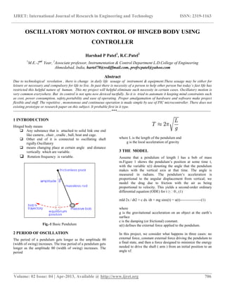
IJRET: International Journal of Research in Engineering and Technology ISSN: 2319-1163
__________________________________________________________________________________________
Volume: 02 Issue: 04 | Apr-2013, Available @ http://www.ijret.org 706
OSCILLATORY MOTION CONTROL OF HINGED BODY USING
CONTROLLER
Harshad P Patel1
, R.C.Patel2
1
M.E.-2nd
Year, 2
Associate professor, Instrumentation & Control Department L.D.College of Engineering
Ahmedabad, India, hartel70@rediffmail.com, profrcpatel@yahoo.com
Abstract
Due to technological revolution , there is change in daily life usuage of instrument & equipment.These usuage may be either for
leisure or necessary and compulsory for life to live. In past there is necessity of a person to help other person but today`s fast life has
restricted this helpful nature of human. This my project will helpful eliminate such necessity in certain cases. Oscillatory motion is
very common everywhere. But its control is not upto now deviced tactfully. So it is tried to automate it keeping mind constraints such
as cost, power consumption, safety,portability and ease of operating. Proper amalgamation of hardware and software make project
flexible and stuff. The repetitive , monotonous and continuous operation is made simple by use of PIC microcontroller. There does not
existing prototype or research paper on this subject. It probable first in it type.
--------------------------------------------------------------------------------***-----------------------------------------------------------------------------
1 INTRODUCTION
Hinged body means
 Any substance that is attached to solid link one end
like camera , chair , cradle , ball, boat and cage.
 Other end of it is connected to oscillating shaft
rigidly.Oscillatory
 means changing place at certain angle and distance
vertically which are variable.
 Rotation frequency is variable.
Fig.-1 Basic Pendulum
2 PERIOD OF OSCILLATION
The period of a pendulum gets longer as the amplitude θ0
(width of swing) increases. The true period of a pendulum gets
longer as the amplitude θ0 (width of swing) increases. The
period
where L is the length of the pendulum and
g is the local acceleration of gravity
3 THE MODEL
Assume that a pendulum of length l has a bob of mass
m.Figure 1 shows the pendulum’s position at some time t,
with the variable x(t) denoting the angle that the pendulum
makes with the vertical axis at that time. The angle is
measured in radians. The pendulum’s acceleration is
proportional to the angular displacement from vertical; we
model the drag due to friction with the air as being
proportional to velocity. This yields a second-order ordinary
differential equation (ODE) for t ≥0:, (1)
mld 2x / dt2 + c dx /dt + mg sinx(t) = u(t)-----------------(1)
where
g is the gravitational acceleration on an object at the earth’s
surface
c is the damping (or frictional) constant.
u(t) defines the external force applied to the pendulum.
In this project, we consider what happens in three cases: no
external force, constant external force driving the pendulum to
a final state, and then a force designed to minimize the energy
needed to drive the shaft ( arm ) from an initial position to an
angle xf.

__________________________________________________________________________________________
4. THE SHAFT (ARM) STABILITY AND
CONTROLLABILITY
The solution to Equation 1 depends on relations among m, c,
g, and u(t) and ranges from fixed amplitude oscillations for the
undamped case (c = 0) to decays (oscillatory or strict) for the
damped case (c > 0). Unfortunately, there is no simple
analytical solution to the pendulum equation in terms of
elementary functions unless we linearize the term sin(x(t)) in
Equation 1 as x(t), an approximation that is only valid for
small values of x(t). Despite the linear approximation’s
limitations, the linearization helps us find analytical solutions
and also apply the results of linear control theory to the
specific problem of robot arm control. To control the arm in a
reasonable way, the system must be stable. Problem 1
considers the stability of a simpler model, valid for small
oscillations. Equation 1’s stability is more difficult to analyze
than the stability of the linearized approximation to it.
Liapunov’s stability occurs when the total energy of an
unforced (or undriven),dissipative mechanical system
decreases as the system state evolves in time. Therefore, the
state vector yT = [x(t), dx(t)/dt] approaches a constant value
(or steady state) corresponding to zero energy as time
increases.According to Liapunov’s formulation, the
equilibrium point y = 0 of a system described by the equation
y′= f(t, y) is globally asymptotically stable if lim t -> ∞
&y(t) = 0 for any choice of y(0). Let y’=f(t, y) and let y
be a steady-state solution of this differential equation.
Terminology varies from text to text, but we will use these
definitions:
A positive definite Liapunov function v at –y(t) is a
continuously differentiable function into the set of
nonnegative numbers. It satisfies
v(–y) = 0, v(y(t)) > 0, and dv(y(t)) / d(t) < 0
for all t > 0 and all y in a neighborhood of –y.
An invariant set is a set for which the solution to the
differential equation remains in the set when the initial state is
in the set. This version of the Liapunov theorem3 for global
asymptotic stability guides our analysis:
Theorem 1. Suppose v is a positive definite Liapunov
function for a steady-state solution –y of y′=f(t, y). Then –y
is stable. If in addition
{y : dv(y(t))/dt = 0} contains no invariant sets other than – y,
then –y is asymptotically stable.
Finding a Liapunov function for a given problem can be
difficult, but success yields important information. For
unstable systems, small perturbations in the application of the
external force can cause large changes in the behavior of the
equation’s solution and, thus, to the pendulum’s behavior, so
the robot arm might behave erratically. Therefore, in practice,
we must ensure that the system is stable
5. NUMERICAL SOLUTION OF INITIAL VALUE
PROBLEM
Next, we develop some intuition for the behavior of the
original and the linearized models by comparing them under
various experimental conditions. For the numerical
investigations assume that m = 1kg, l = 1 m, and g = 9.81
m/sec2, with c = 0 for the undamped case and c = 0.5 kg-
m/sec for the damped case. First we investigate the effects of
damping and of applied forces.
Missing Data: Solution of the Boundary Value
Problem
we solved the initial value problem, in which values of x and
dx/dt were given at time t = 0. In many cases,we don’t have
the initial value for dx/dt, because this value might not be
observable. The missing initial condition prevents us from
applying standard methods to solve initial value problems.
Instead, we might have the value x(tB) = xB at some other
time tB. Next we investigate two solution methods for this
boundary value problem: the shooting method and the finite-
difference method. The idea behind the shooting method is to
guess at the missing initial value z = dx(0)/dt, integrate
Equation 1 using our favorite method, and then use the results
to improve the guess. To do this systematically, we use a
nonlinear equation solver to solve the equation p(z) =xz(tB) –
xB = 0, where xz(tB) is the value reported by an initial value
problem ODE solver for x(tB), given the initial condition z =
dx(0)/dt.
The finite-difference method is an alternate method to solve a
boundary value problem. Choose a small time increment b > 0
and replace the first derivative in the linearized model of
Equation 1 by
dx(t) /dt ={ x(t+b) –x(t-b) } / 2b
and second derivative by
d2x(t) / dt2 ={ x(t+b) – 2x(t) +x(t-b)} / b2
Let n = tB/b, and write the equation for each value xj = x(jb), j
= 1, …, n – 1. The boundary conditions can be stated as x0 =
x(0), xn = xB. This method transforms the linearized versionof
the second-order differential Equation 1 to a system f n – 1
linear equations with n – 1 unknowns. Assuming the solution
to this linear system exists, we then use our favorite linear
system solver to solve these equations.
6. CONTROLLING THE PENDULUM ARM
we investigate how to design a forcing function that drives the
robot arm from an initial position to some other desired
position with the least expenditure of energy. We measure
energy as the integral of the absolute force applied between

__________________________________________________________________________________________
time 0 and the convergence time tc when the arm reaches its
destination.
we studied one simple mathematical model of a robot arm.
The numerical solution couples techniques borrowed from
linear algebra, ordinary differential equations, optimization,
and control theory. Control of our system involves cost trade-
offs: energy versus time of convergence. It’s worth noting that
stability and control studies of most physical systems (such as
underground seepage, muscle movement, and combustion
reactions) require a combination of analytical and
computational tools, even for quite simple mathematical
models.
7. SYSTEM MODEL DEVELOPMENT
This system is described by a second-order ordinary
differential equation (ODE) for t ≥ 0:,
mld 2x / dt2 + c dx /dt + mg sinx(t) = u(t)
l = length of a pendulum = 21 cm = 0.21m for bearing
mounted shaft
= 18 cm = 0.18m for bush
mounted shaft
m = mass of a bob / hinged body = 75 gram = 0.075 kg.
g = gravitational acceleration = 9.81 m /sec
c = damping (or frictional) constant
u(t) = external force ( unit impulse)applied to the pendulum
Therefore
0.0157 (d 2x / dt2) + c (dx /dt) + 0.735 sin (x(t)) = u(t)
for ζ = 0.1 system to be underdamped ( for bush mounted
shaft)
ζ = 0.04 for bearing mounted shaft
ζ = c / 2(mk)1/2
will give
c = 0.0215 ( bush) and c = 0.0215 (bearing)
and small displacement sinx(t) = x(t)
So system equation / model is
0.0157 (d 2x / dt2) + 0.0215 (dx /dt) + 0.735 (x(t)) = u(t)
(bush mounted)
0.0157 (d 2x / dt2) + 0.0083 (dx /dt) + 0.735 (x(t)) = u(t)
(gear mounted)
Compare this equation with standard 2nd order equation
M(dx2/dt2) + F(dx/dt) + dx/dt = u(t)
we get M = 0.0157 F= 0.0215 and K= 0.735
From above equation value of natural frequency oscillation
and damped frequency of oscillation can be calculated
WN= (3K/2M )1/2 = (2.2/0.0314) ½=(70.06) ½ = 8.37
2πFN=1.087 therefore FN=1.33 Hz
7.1 MATLAB SIMULATION RESULT (BEARING
MOUNT)
Fig. 7.1 2nd Order System bearing mount Response
7.2 MATLAB SIMULATION RESULT (BUSH
MOUNT)
Fig. 7.2 2nd Order System bush mount Response

__________________________________________________________________________________________
8 BLOCK DIAGRAM OF SYSTEM
9 METHOD OF COUPLING
1. Rigid coupling
2. Flexible coupling
9.1 RIGID COUPLING
Fig -3 Types of rigid coupling
Rigid couplings which do not allow for any shaft
misalignment. Top: The coupling on the left uses square keys
to transmit torque,the one on the right depends on
compressing rubber sleeves and may therefore allow slip to
occur if the machine becomes overloaded. Lower: Couplings
in the lower group are in two halves and are able to be slipped
over the two shafts after machines have been placed in
position, whereas those in the top group have to be slide onto
their shafts before the machines are positioned.
9.2. FLEXIBLE COUPLING
9.2.1. Belt Drives
A belt drive is used to transmit power from one shaft to
another. The drive is transmitted by a continuous flexible belt
which runs on pulleys mounted on the two shafts. Belt drives
have a number of advantages in some circumstances,
including the ability to transmit power between shafts whose
centers are some distance apart. Speed changes are also
readily achieved, installation and maintenance costs are
relatively low, and no lubrication is needed.
Fig.4 Belt drives

__________________________________________________________________________________________
Characteristics of belt drives
 Belt drives are suitable for medium to long centre distances.
Compare with gears, which are suitable only for short centre
distances.
 Belt drives have some slip and creep (due to the belt
extending slightly under load) and therefore do not have an
exact drive ratio.
 Belts provide a smooth drive with considerable ability to
absorb shock loading.
 Belt drives are relatively cheap to install and to maintain. A
well-designed belt drive has a long service life.
 No lubrication is required. In fact, oil must be kept off the
belt.
 Belts can wear rapidly if operating in abrasive (dusty)
conditions.
9.2.2 Chain Drives
There are similarities between chain drives and belt drives,
and many of the operating principles apply to both. The
analysis of speed and torque relationships developed above for
belts apply equally to chain drives, always working with pitch
line velocities or their equivalent. A simple roller chain drive
used in an automotive application. The chain and sprockets
would be encased within a cover or housing as part of the
engine to maintain cleanliness and to provide lubrication. In
this layout, shaft centres are fixed. Note the use of a chain
tensioner to prevent excessive deflection or “whipping” of the
slack side of the chain.
Fig.-5 Chain drive
Characteristics of chain drives
 Chains provide a positive drive suitable for use where
timing/phasing is required. Before the development of timing
belts, chains were frequently used for driving the camshafts of
motor car engines.
 Chains transmit shock loading, whereas belts tend to absorb
any shock loading which may occur.
 The speedratio is determined by the number of teeth on the
two chain wheels or sprockets, although calculations based on
sprocket pitch diameters and pitch line velocities are equally
valid.
 A chain drive is more costly to set up than a belt drive, but
has a long life.
 Very high torques may be transmitted by chains, beyond the
capacity of belt drives. The drive does not depend on friction.
 Chains generally require lubrication and a heavy duty chain
drive may require a sealed housing incorporating either bath or
jet lubrication, thereby increasing cost.
 Abrasive material rapidly destroys a chain drive.
 It is best not to use chain drives on very long centre
distances because the long lengths of chain tend to “whip”.
9.2.3 Cam and Follower
Fig-6 Elements of Cam-follwer system
Cams are used for essentially the same purpose as linkages,
that is, generation of irregular motion. Cams have an
advantage over linkages because cams can be designed for
much tighter motion specifications. In fact, in principle, any
desired motion program can be exactly reproduced by a cam.
Cam design is also, at least in principle, simpler than linkage
design, although, in practice, it can be very laborious.
Automation of cam design using interactive computing has
not, at present, reached the same level of sophistication as that
of linkage design.A cam and follower system is
system/mechanism that uses a cam and follower to create a
specific motion. The cam is in most cases merely a flat piece
of metal that has had an unusual shape or profile machined
onto it. This cam is attached to a shaft which enable it to be
turned by applying a turning action to the shaft. As the cam
rotates it is the profile or shape of the cam that causes the
follower to move in a particular way. The movement of the
follower is then transmitted to another mechanism or another
part of the mechanism.
If we examine the image below we can see how the profile of
the cam imparts a particular motion on the follower.

__________________________________________________________________________________________
Fig.-7 Types of cam & follower
10. HORIZONTAL SHAFT MOUNTING
METHODS
There are two type of basic methods are used for shaft
mounting.
10.1. Bearing supported
10.2. Bush supported
10.1 Bearing supported
Fig.8 Bearing supported shaft
10.2 Bush supported
Fig.-9 Bush supported shaft
10.3. Different type and size of bush
Fig.10 Types of Bushes
10.4 MATLAB SIMULATION RESULT (BEARING
MOUNT)
Fig. 11 2nd Order System bearing mount Response
10.2 MATLAB SIMULATION RESULT (BUSH
MOUNT)
Fig. 12 2nd Order System bush mount Response

__________________________________________________________________________________________
10.3 VARIOUS METHOD OF SHAFT COUPLING
RESPONSE TO UNIT IMPULSE
10.3.1 Rigidly coupled shaft Response.
10.3.2 Chain / Belt coupled shaft Response
10.3.3 Gear coupled shaft Response.
10.3.4 Cam coupled shaft Response.
11. SYSTEM IMPLEMENTED

__________________________________________________________________________________________
CONCLUSIONS
It was found that the implementation of such a system is better
suited to for deep sleep of infants which causing higher
growth & make his/her mother free for other work, to
smoothen picture & serial director’s shooting work,to
discontinuous heating of substances in industry,to
handicapped ( specifically without two legs),old person and
sick person to swing on their own and at lastto people to get
rid of tyranny heat of summer season economically.
REFERENCES
[1].Institute of Electrical and Electronics Engineers Cannon,
B.L. “Magnetic Resonant Coupling As a Potential Means for
Wireless Power Transfer to Multiple Small Receivers.”Power
Electronics, IEEE Transactions on 24.7 (2009): 1819-1825. ©
2009
[2].Mechanism Design, Analysis and Synthesis by Erdman
and sander, fourth edition, Prentice- Hall, 2001,
[3].Machines and Mechanisms by Uicker, Pennock and
Shigley, third edition, Oxford, 2002.Machines and
Mechanisms by Myszka, Prentice-Hall, 1999
[4].www.SIP-Scootershop.com
[5].www.hondaforeman.com
[6].Kajima, H.; Masahiro Doi; Hasegawa, Y.; Fukuda, T.; ,
"Energy Based Swing Control of a Brachiating Robot,"
Robotics and Automation, 2005. ICRA 2005. Proceedings of
the 2005 IEEE International Conference on , vol., no., pp.
3670- 3675, 18-22 April 2005
[7].K.J. Astrom , K. Furuta,”Swinging up a pendulum by
energy control” Automatica 36 (2000) 287-295
[8].Lu, Cheng-Hsing; Luo, Ching-Hsing; Chen, Yung-Jung;
Yeh, Tsu-Fuh; , "An automatic swinging instrument for better
neonatal growing environment," Review of Scientific
Instruments , Vol. 68, no. 8, pp. 3192-3196, Aug 1997
[9].Piccoli, B. & Kulkarni, J . “Pumping a swing by standing
and squatting: do childrenPump time optimally?”Control
Systems, IEEE, 2005,25,48 – 56
[10].Sato, M.; Toda, M.; , "Motion control of an oscillatory-
base manipulator in the global coordinates," Control and
Automation, 2009. ICCA 2009. IEEE International
Conference on , vol., no., pp.349-354, 9-11 Dec. 2009.

Oscillatory motion control of hinged body using controller

Empfohlen

Empfohlen

Weitere ähnliche Inhalte

Was ist angesagt?

Was ist angesagt? (19)

Andere mochten auch

Andere mochten auch (19)

Ähnlich wie Oscillatory motion control of hinged body using controller

Ähnlich wie Oscillatory motion control of hinged body using controller (20)

Mehr von eSAT Journals

Mehr von eSAT Journals (20)

Kürzlich hochgeladen

Kürzlich hochgeladen (20)

Oscillatory motion control of hinged body using controller