The document discusses load flow studies in power systems. Load flow analysis is important for planning future expansion and determining optimal operation of existing power systems. It provides key information like voltage magnitude and phase angle at each bus and real and reactive power flows. Bus classification depends on which quantities are specified - P,Q buses specify real and reactive power, P,V buses specify real power and voltage magnitude, and the slack bus specifies voltage magnitude and phase angle. Nodal admittance matrix formulation and numerical load flow examples are also presented.
1. Akhilesh A Nimje, Associate Professor, Electrical Engineering, Institute of Technology, Nirma University, Ahmedabad 1
Load Flow Studies
Importance of Load Flow Studies:
The great importance of load flow studies is in the planning the future expansion of the
power system as well as in determining the best operation of the existing systems. The
principle information obtained from load flow studies are the magnitude and phase angle
of the voltage at each bus and the real and reactive power flowing in each line. This
information is essential for the continuous monitoring of the current state and to have a
close look for the scope of the future expansion to meet the increased load demand.
With the advent of the fast and large size digital computers, all kinds of the power
system studies, including load flow can be carried out conveniently. The load flow solution
is an essential tool for designing a new power system and modifying or improving the
performance of the existing ones.
Load flow solutions for a power network can be worked out under balanced and
unbalanced conditions. For such a system, a single-phase representation is adequate. It
requires following steps.
1) Formulation of the network equations
2) Mathematical technique for solution of the equations.
Bus Classification:
In a power system, each bus or node is associated with four quantities, real and reactive
powers, bus voltage magnitude and its phase angle. In a load flow solution, two of the four
quantities are specified and the remaining two are obtained through the solution of the
equations. Depending upon which quantities have been specified, the buses are classified
in the following three categories.
1) Load bus (P,Q bus)
2) Generator bus or Voltage controlled bus (P,V bus)
3) Slack or swing or reference bus (V, bus)
Load bus (P,Q bus)
Real and reactive powers are specified and it is desired to find out the voltage magnitude
and its phase angle. At the load bus, voltage can be allowed to vary within the permissible
tolerance of 5%.
Generator bus or voltage controlled bus (P,V bus)
Here the magnitude of the voltage corresponding to generation voltage and the real power
PG are specified. It is required to find out the reactive power generation QG and the phase
angle of the bus voltage.
Slack Bus or reference bus or swing bus
The magnitude of the voltage and its phase angle are specified. The real and reactive
powers are required to be found out i.e. PG & QG respectively. The phase angle of the
voltage at the slack bus is usually taken as reference. In the analysis, the real and reactive
component of the voltage at a bus are taken as independent variables for the load flow
equations i.e. Vi I = ei + j fi where ei & fi are the real and reactive components
of the voltage at the ith
bus.
2. Akhilesh A Nimje, Associate Professor, Electrical Engineering, Institute of Technology, Nirma University, Ahmedabad 2
Nodal Admittance Matrix (Network Model Formulation)
133112211111312111 )()(
1
yVVyVVyVIIII
nodeAt
)1(][ 13312213121111 yVyVyyyVI
1313121213121111
11
1331221111
;;
1tanarg
yYyYyyyY
busofceadmitingchshunty
YVYVYVI
Similarly, the nodal current equations at bus 2 and bus 3 can be written as follows:
)2(2332222112 YVYVYVI
&
)3(3333223113 YVYVYVI
In Matrix form
)(
3
2
1
333231
232221
131211
3
2
1
A
V
V
V
YYY
YYY
YYY
I
I
I
or in compact form, these equations can be written as
busesthreefortopVYI
q
qpqP
3
1
31,
n
q
qpqp npVYI
busesofnumbernforgeneralIn
1
................3,2,1,
I1 I2
I3
I13
I32
I23
I22
I31
I33
I21I12
I11
1
3
2
y12 = y21
y32 = y23y13 = y31
Three Bus System
3. Akhilesh A Nimje, Associate Professor, Electrical Engineering, Institute of Technology, Nirma University, Ahmedabad 3
nnnnn
n
n
n V
V
V
YYY
YYY
YYY
I
I
I
formmatrixinor
'
'
'''''
'''''
'
'
2
1
21
22221
11211
2
1
A nodal admittance matrix is a square matrix i.e. a few number of elements are non-zero
for an actual power system.
The nodal admittance matrix for the system is as follows:
555451
45444341
343332
232221
15141211
00
0
00
00
0
YYY
YYYY
YYY
YYY
YYYY
Ypq
Where
1514121111 yyyyY
21122112 yyYY
41144114 yyYY
51155115 yyYY
23212222 yyyY
32233223 yyYY
34323333 yyyY
~
~
4
5
2
3
1
y12 = y21
y15 = y51
y45 = y54
y34 = y43
y23 = y32
y14 = y41
4. Akhilesh A Nimje, Associate Professor, Electrical Engineering, Institute of Technology, Nirma University, Ahmedabad 4
43344334 yyYY
4541434444 yyyyY
54455445 yyYY
54515555 yyyY
NOTE: This Y bus matrix can be easily written just by inspection.
NUMERICAL PROBLEM 1
Find YBUS for the system shown below when dotted line is not connected and when it is
connected. Shunt admittances at all buses are neglected.
The following table gives the line impedance identified by the buses on which it terminates.
Solution:
62
15.005.0
111
121212
12 j
jjxrz
y
31
3.01.0
111
131313
13 j
jjxrz
y
2666.0
45.015.0
111
232323
23 j
jjxrz
y
31
3.01.0
111
242424
24 j
jjxrz
y
62
15.005.0
111
343434
34 j
jjxrz
y
Line
Bus to Bus
r, pu x, pu
1-2 0.05 0.15
1-3 0.1 0.3
2-3 0.15 0.45
2-4 0.1 0.3
3-4 0.05 0.15
1 2
3 4
5. Akhilesh A Nimje, Associate Professor, Electrical Engineering, Institute of Technology, Nirma University, Ahmedabad 5
The YBUS matrix for a four-bus system in general is
44434241
34333231
24232221
14131211
YYYY
YYYY
YYYY
YYYY
YBUS
42433424
343432312313
24232423
1313
0
0
00
yyyy
yyyyyy
yyyy
yy
YBUS
9362310
6211666.32666.031
312666.05666.10
031031
jjj
jjjj
jjj
jj
YBUS
If line 1-2 is connected, only Y11,Y22, Y12 & Y21 will change
Therefore
42433424
343432312313
242312242312
13121213
0
0
yyyy
yyyyyy
yyyyyy
yyyy
YBUS
Y11(new) = Y11(old) + y12 = 1 – j 3 + (2 – j 6) = 3 – j 9.
Y22(new) = Y22(old) + y12 = 1.666 – j 5 + (2 – j 6) = 3.666 – j 11
Y12(new) = Y12(old) - y12 = 0 - (2 – j 6) = -2 + j 6.
The modified YBUS with line 1-2 connected is as follows:
Line
Bus to Bus
g, pu b, pu
1-2 2 -6
1-3 1 -3
2-3 0.666 -2
2-4 1 -3
3-4 2 -6
6. Akhilesh A Nimje, Associate Professor, Electrical Engineering, Institute of Technology, Nirma University, Ahmedabad 6
9362310
6211666.32666.031
312666.011666.362
0316293
jjj
jjjj
jjjj
jjj
YBUS
Numerical Problem 2
1) Find the bus incidence matrix [A] for the system shown in fig. Take ground as
reference.
2) Find the primitive admittance matrix [Y]. It is given that all the lines are
characterised by a series impedance of 0.1 + j 0.7 ohms per kilometer and a shunt
admittance of j0.35x10-5
mho per kilometer. Lines are rated at 220 KV
3) Find the bus admittance matrix using singular transformation. Use base values
220 KV and 100 MVA. Express all impedance and admittance in per unit.
4) Also find YBUS by inspection method.
Solution:
Network Graph
1 2
3
4
Oriented Graph
1 2
3
4
120 km
100 km
150 km
100 km110 km
1 2
3 4
7. Akhilesh A Nimje, Associate Professor, Electrical Engineering, Institute of Technology, Nirma University, Ahmedabad 7
The primitive admittance matrix for the system is given by
Tree
1 2
3
41 2
3
4
5
6
7
8
9
node
elements
Element
Element
8. Akhilesh A Nimje, Associate Professor, Electrical Engineering, Institute of Technology, Nirma University, Ahmedabad 8
484
10100
)10220(
)(
/
6
3
2
x
x
VABase
VoltageBase
VoltageBaseVABase
VoltageBase
currentBase
VoltageBase
impedanceBase
mhox
pedanceBase
ceAdmitBase 3
10066115.2
484
1
Im
1
tan
Line impedance per kilometer = 0.1 + j 0.7 ohms
ValueBase
ValueActualj
unitperinkilometerperimpedanceLine
484
7.01.0
=2.066115 x 10⁻⁴
+ j 1.44628 x 10⁻³
pu
puj
xjxZkmforlineforimpedanceLine
144628.00206611.0
]1044628.110066115.2[10010021 34
12
pujZkmforlineforimpedanceLine 15909.002272.011031 13
pujZkmforlineforimpedanceLine 216942.003099165.015041 14
pujZkmforlineforimpedanceLine 144628.00206611.010042 24
pujZkmforlineforimpedanceLine 1735536.00247933.012043 34
puj
j
y 776.6968.0
87.81146096.0
1
144628.00206611.0
1
012
puj
j
y 16.688.0
87.8116070495.0
1
1590908.002272.0
1
013
puj
j
y 5174.464533.0
87.8121914.0
1
216942.003099165.0
1
014
puj
j
y 776.6968.0
87.81146096.0
1
144628.00206611.0
1
024
puj
j
y 6466.580665.0
87.811753156.0
1
1735536.00247933.0
1
034
Line charging admittance per km = j0.35 x 10-5
mho/km
Line charging Admittance per km in per unit = j0.35 x 10-5
/ 2.06615 x 10-3
= j1.6939 x 10-3
pu.
9. Akhilesh A Nimje, Associate Professor, Electrical Engineering, Institute of Technology, Nirma University, Ahmedabad 9
1
pqy pu 2/1
pqy pu
Line charging admittance for line 1-2 (100 km) j0.16939 j0.084695
Line charging admittance for line 1-3 (110 km) j0.186336 j0.093168
Line charging admittance for line 1-4 (150 km) j0.254 j0.127
Line charging admittance for line 2-4 (100 km) j0.16939 j0.084695
Line charging admittance for line 3-4 (120 km) j0.2032 j0.1016
Computing the parameters of Primitive admittance matrix
𝑦10 = 𝑗(0.08469 + 0.127 + 0.09316) = 𝑗0.3048
𝑦20 = 𝑗(0.08469 + 0.084695) = 𝑗0.16939
𝑦30 = 𝑗(0.09316 + 0.1016) = 𝑗0.1947
𝑦40 = 𝑗(0.1016 + 0.127 + 0.08469) = 𝑗0.31329
The primitive admittance matrix is as follows:
14
24
34
13
12
40
30
20
10
][
y
y
y
y
y
y
y
y
y
Y
1 2
3 4
y12 = 0.908-j6.776
y14 = 0.6453-j4.5174
y34 = 0.80665-j5.6466
y24 = 0.968-j6.776
y13 = 0.88-j6.16
J0.1016
J0.093168
J0.093168
J0.084695 J0.084695
J0.127
J0.127
J0.084695
J0.084695J0.1016
10. Akhilesh A Nimje, Associate Professor, Electrical Engineering, Institute of Technology, Nirma University, Ahmedabad 10
51.4
645.0
00000000
0
77.6
968.0
0000000
00
64.5
806.0
000000
00016.688.000000
000077.6968.00000
00000313.0000
000000194.000
0000000169.00
00000000304.0
j
j
j
j
j
j
j
j
j
Y
YBUS = AT
YA
517.4645.000517.4645.0
776.6968.00776.6968.00
646.5806.0646.5806.000
016.688.0016.688.0
0077.6968.077.6968.0
313.0000
0194.000
00169.00
000304.0
]][[
jj
jj
jj
jj
jj
j
j
j
j
AY
62.1642.2646.5806.0776.6968.051.4645.0
646.5806.061.1168.1016.688.0
776.6968.0038.1393.1774.6968.0
51.4645.016.688.0774.6968.014.1749.2
jjjj
jjj
jjj
jjjj
YBUS
Load Flow Problem
The complex power injected by the source into ith
bus of a power system is
Si = Pi + jQi = Vi Ji
*
i = 1, 2, ……….n (1)
Where Vi is the voltage at ith
bus with respect to ground and Ji is the source current
injected into the bus.
The load flow problem is handled more conveniently if we use Ji rather than Ji
*
.
Therefore taking the complex conjugate of equation (1), we have
Pi –jQi = Vi
*
Ji i = 1,2,………………n (2)
As I = YV
At any particular node
11. Akhilesh A Nimje, Associate Professor, Electrical Engineering, Institute of Technology, Nirma University, Ahmedabad 11
I1 = V1Y11 + V2Y12 + V3Y13
In general
n
k
kiki niVYJ
1
................,2,1
Substituting value of Ji in equation (2), we get
n
k
kikiii niVYVjQP
1
*
.................,2,1
Equating real & imaginary parts
)3..(........................................Re)(Re
1
*
n
k
kikii VYVPoweralP
)4..(........................................Im)(Re
1
*
n
k
kikii VYVpoweractiveQ
iki j
ikik
j
i eYYeVVformpolarIn
||&||
The real & reactive powers can be expressed as
n
k
ikikikkii niCosYVVpowerrealP
1
)5(................2,1)(||||||)(
n
k
ikikikkii niSinYVVpowerreactiveQ
1
)6(................2,1)(||||||)(
APPROXIMATE LOAD FLOW SOLUTION
Assumptions:
1) The line resistance is negligible. Since line resistance is small as compared to its
reactance, therefore it can be neglected. Thus the active power loss is zero.
2) This gives ik 90o
& ii -90o
and i - k is small below 30o
so that sin(i - k)
(i - k)
Therefore equation (5) and (6) reduces to
𝑃𝑖 = |𝑉𝑖| ∑{|𝑉𝑘||𝑌𝑖𝑘| 𝑐𝑜𝑠[90 − (𝛿𝑖 − 𝛿 𝑘)] + |𝑉𝑖||𝑌𝑖𝑖| 𝑐𝑜𝑠[−90 − (𝛿𝑖 − 𝛿𝑖)]}
𝑛
𝑘=1
𝑃𝑖 = |𝑉𝑖| ∑{|𝑉𝑘||𝑌𝑖𝑘| sin(𝛿𝑖 − 𝛿 𝑘) − |𝑉𝑖||𝑌𝑖𝑖| 𝑠𝑖𝑛(𝛿𝑖 − 𝛿𝑖)}
𝑛
𝑘=1
𝑠𝑖𝑛𝑐𝑒 𝑠𝑖𝑛 (𝛿𝑖 − 𝛿 𝑘) ≅ (𝛿𝑖 − 𝛿 𝑘)
)7(..........................,3,2;)(||||||
1
niYVVP k
n
ik
k
iikkii
12. Akhilesh A Nimje, Associate Professor, Electrical Engineering, Institute of Technology, Nirma University, Ahmedabad 12
𝑄𝑖 = −|𝑉𝑖| ∑{|𝑉𝑘||𝑌𝑖𝑘| 𝑠𝑖𝑛[90 − (𝛿𝑖 − 𝛿 𝑘)] + |𝑉𝑖||𝑌𝑖𝑖| 𝑠𝑖𝑛[−90 − (𝛿𝑖 − 𝛿𝑖)]}
𝑛
𝑘=1
𝑄𝑖 = −|𝑉𝑖| ∑{|𝑉𝑘||𝑌𝑖𝑘| cos(𝛿𝑖 − 𝛿 𝑘) − |𝑉𝑖||𝑌𝑖𝑖| cos(𝛿𝑖 − 𝛿𝑖)}
𝑛
𝑘=1
)8(...............,3,2;||||)(|||||| 2
1
niYVCosYVVQ iiik
n
ik
k
iikkii
3) All buses other than the slack are PV buses i.e. voltage magnitude of all the buses
including the slack bus are specified.
NUMERICAL PROBLEM 3
Consider a four-bus sample power system wherein line reactances are indicated in per unit.
Line resistances are considered negligible. The magnitude of all the four bus voltages is
specified to be 1.0 pu. The bus powers are specified in the table below.
Bus Real Demand Reactive
Demand
Real Generation Reactive Generation
1 PD1 = 1.0 QD1 = 0.5 PG1 = ? QG1(unspecified)
2 PD2 = 1.0 QD2 = 0.4 PG2 = 4.0 QG2(unspecified)
3 PD3 = 2.0 QD3 = 1.0 PG3 = 0 QG3(unspecified)
4 PD4 = 2.0 QD4 = 1.0 PG4 = 0 QG4(unspecified)
Solution:
Generation = Demand + Losses
But since resistance is negligible, it is a loss less line.
Therefore
PG1 + PG2 + PG3 + PG4 = PD1 + PD2 + PD3 + PD4
PG1 + 4.0 + 0 + 0 = 1.0 + 1.0 + 2.0 + 2.0
G1 G3
G2G4
S1=1.0+jQ1 S3 = -2+jQ3
S4 = -2+jQ4
S2 = 3+jQ2
1 3
4 2
|V1| = 1.0 |V3| = 1.0
|V4| = 1.0 |V2| = 1.0
J0.15
J0.2
J0.15
J0.1 J0.1
14. Akhilesh A Nimje, Associate Professor, Electrical Engineering, Institute of Technology, Nirma University, Ahmedabad 14
for i = 4
)3......(..............................267.1667.610
)(67.6)(100.12
)(||||)(||||)(||||||
421
2414
34433244221441144
YVYVYVVP
If bus ‘1’ is considered as reference, 1 = 0.
Solving equation 1, 2 & 3 we get,
2 = 0.077 rad = 4.41o
; 3 = -0.074 rad = -4.23o
; 4 = -0.089 rad = -5.11o
.
The bus voltages are now updated as follows:
𝑉1 = 1.0 0 𝑜
𝑝𝑢; 𝑉2 = 1.0 4.41 𝑜
𝑝𝑢;
𝑉3 = 1.0 −4.23 𝑜
𝑝𝑢; 𝑉4 = 1.0 − 5.11 𝑜
𝑝𝑢;
Again
.......,..........,3,2,1;||||)(|||||| 2
1
niYVCosYVVQ iiiki
n
ik
k
ikkii
The above equation is required to find the reactive power generation at each bus using
QGi = Qi + QDi
Thus
For i = 1
.0727.067.21)11.5(10)23.4(67.6)41.4(50.1
||||)(||||)(||||)(||||||
1
11
2
141144311332112211
puCosCosCosQ
YVCosYVCosYVCosYVVQ
for i = 2
.2202.067.21)11.541.4(67.6)23.441.4(10)41.4(50.1
||||)(||||)(||||)(||||||
2
22
2
242244322331221122
puCosCosCosQ
YVCosYVCosYVCosYVVQ
for i = 3
.132.067.16)41.423.4(10)23.4(67.60.1
||||)(||||)(||||)(||||||
3
33
2
343344233221331133
puCosCosQ
YVCosYVCosYVCosYVVQ
for i = 4
.132.067.16)41.411.5(67.6)11.5(100.1
||||)(||||)(||||)(||||||
4
44
2
434433244221441144
puCosCosQ
YVCosYVCosYVCosYVVQ
Reactive Power Generation
QG1 = Q1 + QD1 = 0.0727 + 0.5 = 0.5727 pu
QG2 = Q2 + QD2 = 0.2202 + 0.4 = 0.6202 pu
QG3 = Q3 + QD3 = 0.1320 + 1.0 = 1.1320 pu
QG4 = Q4 + QD4 = 0.1320 + 1.0 = 1.1320 pu
15. Akhilesh A Nimje, Associate Professor, Electrical Engineering, Institute of Technology, Nirma University, Ahmedabad 15
Reactive Line Losses = [QG1+QG2+QG3+QG4] - [QD1+QD2+QD3+QD4] = 0.5569 pu.
Since |Z| X therefore = 90o
, the line flows can be written as
)(
||||
ki
ik
ki
kiik Sin
X
VV
PP
where Pik is the real power flow from bus ‘i’ to bus ‘k’
Using Approximate load flow solution
.492.0))23.4(0(
15.0
1
)(
||||
31
13
31
3113 puSinSin
X
VV
PP
.3844.0))41.40(
2.0
1
)(
||||
21
12
21
2112 puSinSin
X
VV
PP
.8906.0))11.5(0(
1.0
1
)(
||||
41
14
41
4114 puSinSin
X
VV
PP
.502.1)41.423.4(
1.0
1
)(
||||
23
32
23
2332 puSinSin
X
VV
PP
.103.1))11.5(41.4(
15.0
1
)(
||||
42
24
42
4224 puSinSin
X
VV
PP
From sending end reactive power as derived earlier in power circle diagram
𝑄𝑠 =
|𝑉𝑠|2
|𝑍|
sin −
|𝑉𝑠||𝑉𝑟|
|𝑍|
𝑠𝑖𝑛(𝜃 + 𝛿)
The reactive power flow for |Z| = X & = 90o
Using Approximate load flow solution
)(
|||||| 2
ki
ik
ki
ik
i
kiik Cos
X
VV
X
V
QQ
where, Qik is the reactive power flow from bus ‘i’ to bus ‘k’.
.018.0
15.0
)23.4(
15.0
1
)(
||||||
31
13
31
13
2
1
3113 pu
Cos
Cos
X
VV
X
V
QQ
.015.0
2.0
)41.4(
2.0
1
)(
||||||
21
12
21
12
2
1
2112 pu
Cos
Cos
X
VV
X
V
QQ
.04.0
1.0
)11.5(
1.0
1
)(
||||||
41
14
41
14
2
1
4114 pu
Cos
Cos
X
VV
X
V
QQ
.1135.0
1.0
)41.423.4(
1.0
1
)(
||||||
23
32
23
32
2
3
2332 pu
Cos
Cos
X
VV
X
V
QQ
.0918.0
15.0
)11.541.4(
15.0
1
)(
||||||
42
24
42
24
2
2
4224 pu
Cos
Cos
X
VV
X
V
QQ
16. Akhilesh A Nimje, Associate Professor, Electrical Engineering, Institute of Technology, Nirma University, Ahmedabad 16
S13 = P13 + j Q13 = 0.492 + j 0.018 (Power flows from bus 1 to bus 3)
S12 = P12 + j Q12 = -0.3844 + j 0.015 (Power flows from bus 2 to bus 1)
S14 = P14 + j Q14 = 0.8906 + j 0.04 (Power flows from bus 1 to bus 4)
S32 = P32 + j Q32 = -1.502 + j 0.1135 (Power flows from bus 2 to bus 3)
S24 = P24 + j Q24 = 1.103 + j 0.0918 (Power flows from bus 2 to bus 4)
Line Flows can be indicated on the system as follows:
Gauss Seidel Method
It is an iterative algorithm for solving a set of non-linear algebraic equations. The iterative
process is then repeated till the solution vector converges. It is assumed that all the buses
other than slack bus are PQ buses. This method is also applicable to PV buses as well.
In a GS method, the slack bus voltages are specified, suppose there are ‘n’ number of buses
in a power system, there will be (n-1) bus voltages, starting values of whose magnitude and
angles are assumed. These values are then updated through the iterative process.
The complex power injected by a source into ith
bus of a power system is
Si = Pi + jQi = Vi Ji
*
i = 1, 2, ……….n (1)
Vi = voltage at ith
bus
Ji = source current injected.
Load flow study is convenient by the use of Ji rather than Ji
*
Taking Complex Conjugate of equation (1)
Pi – jQi = Vi
*
Ji i = 1, 2, ………n (2)
Where
n
k
kiki VYJ
1
1
2
3
4
0.3844+j0.015
0.492+j0.018
0.8906+j0.04
8
1.502+j0.1135
1.103+j0.0918
1+j0.5
2+j1
2+j1
1+j0.4
j1.1322+j0.57
4+j0.62j1.132
17. Akhilesh A Nimje, Associate Professor, Electrical Engineering, Institute of Technology, Nirma University, Ahmedabad 17
Expanding & Rewriting, we get
n
ik
k
kiki
ii
i VYJ
Y
V
1
][
1
But from equation (2), *
i
ii
i
V
jQP
J
)3(......................,3,2
1
1
*
niVY
V
jQP
Y
V
n
ik
k
kik
i
ii
ii
i
Where, the voltages substituted on right hand side of equation (3) are the most recently
calculated (updated) values for the corresponding buses. But slack bus voltage is fixed and
hence it is not updated. The iterations are repeated till no bus voltage magnitude changes.
Such a computation process is called as convergence of the solution.
If PV Buses are also present
At PV bus, P & V are specified whereas Q & are unspecified. Here Q and are updated
using GS method. It includes the following steps
aswrittenbecanequationaboveiteration
rforSideHandRightonvoltagesofvaluerecentmostputtingbyupdatedisQ
VYVQ
Step
th
i
n
k
kikii
,
)1(
Im
1
1
*
1
1
*)1(*
Im
i
k
n
ik
r
kik
r
i
r
kik
r
ii VYVVYVQ
ii
r
iir
i
i
k
n
ik
r
kik
r
kik
r
i
r
i
r
i
r
i
Y
jQP
A
where
VBVB
V
A
ofAngle
VThusstepfromobtainedisofvaluerevisedThe
Step
)1(
)1(
1
1 1
)()1(
*)(
)1(
)1()1(
.1
2
This gives a range of reactive generation, i.e. Qmin to Qmax , If Qi is not within this limit,
that particular ith
bus is then treated as ‘PQ’ bus.
NUMERICAL PROBLEM 4
For the network shown in figure, obtain the complex bus bar voltage at bus 2 at the end of
first iteration. Use GS method. Line impedances shown in figure are in per unit. Bus 1 is a
18. Akhilesh A Nimje, Associate Professor, Electrical Engineering, Institute of Technology, Nirma University, Ahmedabad 18
slack bus with V1 = 1.00o
; P2 + j Q2 = -5.96 + j 1.46 ; |V3| = 1.02 pu. Assume V3
o
=
1.02 0o
; and V2
o
= 1.00o
Solution
53.1169.7
06.004.0
1
12 j
j
y
; 07.2338.15
03.002.0
1
23 j
j
y
Y11 = y12 = 7.69 – j 11.53; Y12 = -y12 = -7.69 + j 11.53 ; Y13 = 0;
Y22 = y21 + y23 = 23.07 – j 34.61; Y23 = -y23 = -15.38 + j 23.07;
Y33 = y32 = 15.38 – j 23.07.
07.2338.1507.2338.150
07.2338.1561.3407.2353.1169.7
053.1169.753.1169.7
jj
jjj
jj
YBUS
0
323
0
121*0
2
22
22
1
2
1
VYVY
V
jQP
Y
V
02.1)07.2338.15()53.1169.7(
)01(
46.196.5
61.3407.23
11
2 jj
j
j
j
V
V2
1
= 0.973 -8.1934o
pu OR 0.963 –j 0.1386 pu.
NUMERICAL PROBLEM 5
For the sample system, the generators are connected to all four buses while loads are at
buses 2 & 3. All buses other than slack bus are PQ type. Assume flat voltage start, find the
voltage and bus angles at other three buses at the end of third GS iteration.
Bus Pi pu Qi pu Vi pu. Remarks
1 - - 1.04 0o Slack bus
2 0.5 -0.2 - PQ bus
3 -1.0 0.5 - PQ bus
4 0.3 -0.1 - PQ bus
Line
Bus to Bus
r, pu x, pu
1-2 0.05 0.15
1-3 0.1 0.3
2-3 0.15 0.45
2-4 0.1 0.3
3-4 0.05 0.15
0.04+j0.06 0.02+j0.03
1 2 3
1 2
3 4
19. Akhilesh A Nimje, Associate Professor, Electrical Engineering, Institute of Technology, Nirma University, Ahmedabad 19
Solution:
62
15.005.0
111
121212
12 j
jjxrz
y
31
3.01.0
111
131313
13 j
jjxrz
y
2666.0
45.015.0
111
232323
23 j
jjxrz
y
31
3.01.0
111
242424
24 j
jjxrz
y
62
15.005.0
111
343434
34 j
jjxrz
y
42433424
343432312313
242312242312
13121213
0
0
yyyy
yyyyyy
yyyyyy
yyyy
YBUS
9362310
6211666.32666.031
312666.011666.362
0316293
jjj
jjjj
jjjj
jjj
YBUS
Using Formula
n
ik
k
kiki
ii
i VYJ
Y
V
1
][
1
where *
i
ii
i
V
jQP
J
bus 1 is a slack bus V1 = 1.04 0 o
= 1.04 + j0.
Initially we shall assume V2
0
= V3
0
= V4
0
= 1 + j 0 and later on after each iteration, they
will be updated.
FIRST ITERATION
0
424
0
323
0
121*0
2
22
22
'
2
1
VYVYVY
V
jQP
Y
V
Line
Bus to Bus
g, pu b, pu
1-2 2 -6
1-3 1 -3
2-3 0.666 -2
2-4 1 -3
3-4 2 -6
20. Akhilesh A Nimje, Associate Professor, Electrical Engineering, Institute of Technology, Nirma University, Ahmedabad 20
pujpu
jjj
j
j
j
V
o
046.00186.1.59.2019.1
)31()266.0(04.1)62(
01
2.05.0
1166.3
1'
2
Note: initially we assumed V2
o
= 1 + j 0 but with the value V2
1
obtained we shall put it in
our upcoming equations.
0
434
'
232
0
131*0
3
33
33
'
3
1
VYVYVY
V
jQP
Y
V
pujpu
jjjj
j
j
j
V
o
087.00273.1.851.4031.1
)62()046.00186.1)(266.0(04.1)31(
01
5.01
1166.3
1'
3
Note: initially we assumed V3
o
= 1 + j 0 but with the value V3
1
obtained we shall put it in
upcoming equations.
'
343
'
242
0
141*0
4
44
44
'
4
1
VYVYVY
V
jQP
Y
V
puj
jjjj
j
j
j
V
00948.002443.1
)087.00273.1)(62()046.00186.1)(31(
01
1.03.0
93
1'
4
SECOND ITERATION
'
424
'
323
0
121*'
2
22
22
''
2
1
VYVYVY
V
jQP
Y
V
pujpu
j
jjjj
j
j
j
V
o
026.002815.1.49.10285.1
)00948.00244.1(
)31()087.00273.1)(266.0(04.1)62(
046.00186.1
2.05.0
1166.3
1''
2
'
434
''
232
0
131*'
3
33
33
''
3
1
VYVYVY
V
jQP
Y
V
pujpu
j
jjjj
j
j
j
V
o
1022.0030.1.662.5036.1
)00948.00244.1(
)62()026.002815.1)(266.0(04.1)31(
087.0027.1
5.01
1166.3
1''
3
''
343
''
242
0
141*'
4
44
44
''
4
1
VYVYVY
V
jQP
Y
V
21. Akhilesh A Nimje, Associate Professor, Electrical Engineering, Institute of Technology, Nirma University, Ahmedabad 21
.488.1031.1026.00311.1
)1022.003.1)(62()026.002815.1)(31(
00948.0024.1
1.03.0
93
1''
4
pupuj
jjjj
j
j
j
V
THIRD ITERATION
''
424
''
323
0
121*''
2
22
22
'''
2
1
VYVYVY
V
jQP
Y
V
pujpu
j
jjjj
j
j
j
V
o
0195.0031.1.083.10319.1
)026.00311.1(
)31()1022.003.1)(266.0(04.1)62(
026.00322.1
2.05.0
1166.3
1'''
2
''
434
'''
232
0
131*''
3
33
33
'''
3
1
VYVYVY
V
jQP
Y
V
pujpu
j
jjjj
j
j
j
V
o
104.00368.1.724.5042.1
)026.00311.1(
)62()0195.0031.1)(266.0(04.1)31(
1022.003.1
5.01
1166.3
1'''
3
'''
343
'''
242
0
141*''
4
44
44
'''
4
1
VYVYVY
V
jQP
Y
V
.7.1031.103.00358.1
)104.00368.1)(62()0195.0031.1)(31(
026.00311.1
1.03.0
93
1'''
4
pupuj
jjjj
j
j
j
V
Acceleration of Convergence
Convergence in GS solution can sometimes be speeded up by the use of the acceleration
factor. For the ith
bus, the accelerated value of voltage at the (r + 1)th
iteration is given by
)()( )()1()()1( r
i
r
i
r
i
r
i VVVdaccelerateV
where is a real number called the acceleration factor. A suitable value of for any system
can be obtained by trial load flow studies. A generally recommended value is = 1.6. A
wrong choice of may indeed slow down convergence or even cause the method to
diverge.
This concludes the load flow analysis for the case of PQ buses only.
NOTE: Powers at load bus are taken as negative and at generator bus they are taken as
positive.
22. Akhilesh A Nimje, Associate Professor, Electrical Engineering, Institute of Technology, Nirma University, Ahmedabad 22
NUMERICAL PROBLEM 6
The load flow data for a four-bus system is given in the table 1 & 2.
Table 1
Table 2
Bus code P Q V Remarks
1 - - 1.06 Slack
2 -0.5 -0.2 1+j0 PQ
3 -0.4 -0.3 1+j0 PQ
4 -0.3 -0.1 1+j0 PQ
i) Determine the voltages at the end of first iteration using GS method. Take = 1.6.
ii) If Bus ‘2’ is taken as a generator bus with |V2| = 1.04 and reactive power constraint is
0.1 Q2 1.0 Determine the voltages starting with a flat profile and assuming
accelerating factor as 1.0. (Take P2 = +0.5 pu when bus 2 is a generator bus)
iii) If the reactive power constraint on generator 2 is 0.2 Q2 1.0. Determine the voltages
starting with a flat profile and assuming accelerating factor as 1.0. (Take P2 = +0.5 pu
when bus 2 is a generator bus)
Solution:
;82;41
;664.2666.0;0;41;82;123
664.14666.3;664.14666.3;123
3424
2314131244
3322131211
pujYpujY
pujYYpujYpujYpujY
pujYpujYpujyyY
12382410
82664.14666.3664.2666.041
41664.2666.0664.14666.382
04182123
:tan
jjj
jjjj
jjjj
jjj
Y
followsasissystemtheforMatrixceAdmitBusThe
BUS
Bus
code
Admittance
1-2 2-j8
1-3 1-j4
2-3 0.666-j2.664
2-4 1-j4
3-4 2-j8
1 2
4
y23 = 0.666-j2.664
y12 = 2-j8
y34 = 2-j8
y24 = 1-j4y13 = 1-j4
3
23. Akhilesh A Nimje, Associate Professor, Electrical Engineering, Institute of Technology, Nirma University, Ahmedabad 23
Computing voltages at different buses other than slack bus
0
424
0
323
0
121*0
2
22
22
'
2
1
VYVYVY
V
jQP
Y
V
puj
jjj
j
j
j
V
02888.001187.1
)41()664.2666.0(06.1)82(
01
2.05.0
664.1466.3
1'
2
V2
1
acc = (1.0 + j 0.0) + 1.6 {(1.01187 – j 0.02888) - (1.0 + j0)}
= 1.01899 – j 0.046208 pu.
0
434
1
232
0
131*0
3
33
33
'
3
1
VYVYVY
V
jQP
Y
V acc
puj
jj
jjj
j
j
j
V
029248.0994119.0
)01)(82(
)046208.001899.1)(664.2666.0(06.1)41(
01
3.04.0
664.1466.3
1'
3
V3
1
acc = (1 + j 0) + 1.6 {(0.994119 – j 0.029248) – (1 + j 0)}
= 0.99059 - j 0.0467968 pu.
accacc
VYVYVY
V
jQP
Y
V 1
343
1
242
0
141*0
4
44
44
'
4
1
puj
jjjj
j
j
j
V
064684.09716032.0
)0467968.099059.0)(82()046208.001899.1)(41(
01
1.03.0
123
1'
4
V4
1
acc = (1 + j 0) + 1.6{(0.9716032 – j 0.064684) – (1 + j 0)}
= 0.954565 – j 0.1034944 pu.
If bus ‘2’ is a PV bus
)1(Im
1
1
*)1(*
i
k
n
ik
r
kik
r
i
r
kik
r
ii VYVVYVQ
Thus for i = 2 ; r = 0;
)2()()()()(Im 0
424
0
323
0
222
*0
2
1
121
*0
22 VYVYVYVVYVQ
It should be noted that V1
1
is equal to V1
0
since it is a slack bus, its voltage is fixed at
1.06 pu. Therefore the above expansion can be simplified as
)3()(Im 0
424
0
323
0
222
0
121
*0
22 VYVYVYVYVQ
Voltage at bus ‘2’ is specified as |V2| = 1.04 pu.
Initial value of 2 = 0o
(Assumed) it will be updated after iterations.
Therefore V2 in its polar form can be written as V2 2 = 1.04 0o
24. Akhilesh A Nimje, Associate Professor, Electrical Engineering, Institute of Technology, Nirma University, Ahmedabad 24
In Rectangular form V2 = 1.04 + j 0 pu. V2
*
= 1.04 – j 0 pu.
Flat Voltage profile is given therefore all the bus voltages are 1 + j 0 i.e.
V3 = V4 = 1 + j 0.
Putting values in equation (3)
0.1)41(
0.1)664.2666.0()004.1)(664.14666.3()06.1)(82(
)004.1(Im2
j
jjjj
jQ
Q2 = 0.1108 pu.
The reactive power limit is specified as 0.1 Q2 1.0
The calculated value of Q2 using equation (3) lies within the specified limit.
Therefore bus ‘2’ is a PV bus i.e. bus ‘2’ is a voltage controlled or generator bus.
Since bus ‘2’ is concluded to be a generator bus, the powers will now be taken as positive
at this bus. i.e. P2 = 0.5 pu (given) ; Q2 = 0.1108 pu (calculated) .
ii
r
iir
i
i
k
n
ik
r
kik
r
kik
r
i
r
i
r
i
r
i
Y
jQP
A
where
VBVB
V
A
ofAngle
VThusobtainedisofvaluerevisedThe
)1(
)1(
1
1 1
)()1(
*)(
)1(
)1()1(
.
424323121*0
2
22
22
2
)(
1
VYVYVY
V
jQP
Y
new
0.1)41(0.1)664.2666.0(06.1)82(
004.1
1108.05.0
664.14666.3
1
2 jjj
j
j
j
new
= 1.0472846 + j0.0291476 pu = 1.04769 1.59o
pu
Thus 2 new = 1.59 o
Therefore voltage at bus ‘2’ in its polar form V2 = 1.04 1.59o
pu
In rectangular form V2 = 1.0395985 + j 0.02891158 pu.
However V3 & V4 can be calculated using conventional method but with new updated
value of V2.
0
434232
0
131*0
3
33
33
1
3
)(
1
VYVYVY
V
jQP
Y
V
)01)(82(
)02891158.00395985.1)(664.2666.0(06.1)41(
01
3.04.0
664.14666.3
11
3
jj
jjj
j
j
j
V
pujV 015607057.09978866.01
3
25. Akhilesh A Nimje, Associate Professor, Electrical Engineering, Institute of Technology, Nirma University, Ahmedabad 25
1
343242
0
141*0
4
44
44
1
4
)(
1
VYVYVY
V
jQP
Y
V
)015607057.09978866.0)(82(
)02891158.00395985.1)(41(
)01(
1.03.0
123
11
4
jj
jj
j
j
j
V
.022336.0998065.01
4 pujV
If reactive power limit on generator 2 is 0.2 Q2 1.0.
In the second part of the problem, Q2 has been calculated as 0.1108 pu which does not lie
within limits specified above. For this, voltage at bus ‘2’ is assumed to be 1 + j0 (Using
flat voltage profile) and will be updated through iterations assuming V3
0
= V4
0
= 1 + j 0
pu. It should also be noted that for a generators bus, powers are taken positive whereas
for a load or PQ bus, powers are taken as negative. Therefore P2 = 0.5 pu and setting Q2
to its minimum limit i.e. Q2 min = 0.2 pu.
0
424
0
323
0
121*0
2
min22
22
1
2
)(
1
VYVYVY
V
jQP
Y
V
)41()664.2666.0(06.1)82(
)01(
2.05.0
664.14666.3
11
2 jjj
j
j
j
V
𝑉2
′
= 1.09822 + 𝑗0.03010 𝑝𝑢
0
434
1
232
0
131*0
3
33
33
1
3
)(
1
VYVYVY
V
jQP
Y
V
)82(
)03010.0098221.1)(664.2666.0(06.1)41(
)01(
3.04.0
664.14666.3
11
3
j
jjj
j
j
j
V
𝑉3
′
= 1.00853 − 𝑗0.01545 𝑝𝑢 = 1.00865 − 0.878 𝑜
𝑝𝑢
1
343
1
242
0
141*0
4
44
44
1
4
)(
1
VYVYVY
V
jQP
Y
V
)015456.000853.1(
)82()030105662.0098221.1)(41(
01
1.03.0
123
11
4
j
jjj
j
j
j
V
𝑉4
′
= 1.0276 − 𝑗0.020082 𝑝𝑢 = 1.0278 − 1.1196 𝑜
𝑝𝑢
NUMERICAL PROBLEM 7
1) For the sample system, the generators are connected to all four buses while loads are at
buses 2 & 3. All buses other than slack bus are PQ type. Assume flat voltage start, find the
26. Akhilesh A Nimje, Associate Professor, Electrical Engineering, Institute of Technology, Nirma University, Ahmedabad 26
voltage and bus angles at other three buses at the end of first GS iteration. Assume Base
MVA 1000
Bus Real Power
Generation
PGi (MW)
Real Power
Demand
PDi (MW)
Reactive Power
Generation QGi
(MVAR)
Reactive Power
Demand
QDi (MVAR)
Vi Remarks
1 - - - - 1.040o Slack
2 700 200 200 400 - PQ
3 200 300 600 100 - PQ
4 400 100 200 300 - PQ
2) Let bus 2 be a PV bus with |V2| = 1.04 pu. Assuming a flat voltage start, find Q2,
2, V3, V4 at the end of first GS iteration. Given : 0.2 Q2 1.
3) Repeat part 2 for reactive power limits as : 0.25 Q2 1.
Solution:
62
15.005.0
111
121212
12 j
jjxrz
y
31
3.01.0
111
131313
13 j
jjxrz
y
2666.0
45.015.0
111
232323
23 j
jjxrz
y
31
3.01.0
111
242424
24 j
jjxrz
y
62
15.005.0
111
343434
34 j
jjxrz
y
Line
Bus to Bus
r, pu x, pu
1-2 0.05 0.15
1-3 0.1 0.3
2-3 0.15 0.45
2-4 0.1 0.3
3-4 0.05 0.15
Line
Bus to Bus
g, pu b, pu
1-2 2 -6
1-3 1 -3
2-3 0.666 -2
2-4 1 -3
3-4 2 -6
1 2
3 4
27. Akhilesh A Nimje, Associate Professor, Electrical Engineering, Institute of Technology, Nirma University, Ahmedabad 27
42433424
343432312313
242312242312
13121213
0
0
yyyy
yyyyyy
yyyyyy
yyyy
YBUS
9362310
6211666.32666.031
312666.011666.362
0316293
jjj
jjjj
jjjj
jjj
YBUS
Using Formula
n
k
k
kiki
ii
i VYJ
Y
V
1
1
][
1
where *
i
ii
i
V
jQP
J
bus 1 is a slack bus V1 = 1.04 0 o
= 1.04 + j0.
Initially we shall assume V2
0
= V3
0
= V4
0
= 1 + j 0 and later on after each iteration, they
will be updated.
FIRST ITERATION
0
424
0
323
0
121*0
2
22
22
'
2
1
VYVYVY
V
jQP
Y
V
pujpu
jjj
j
j
j
V
o
046.00186.1.59.2019.1
)31()266.0(04.1)62(
01
2.05.0
1166.3
1'
2
0
434
'
232
0
131*0
3
33
33
'
3
1
VYVYVY
V
jQP
Y
V
pujpu
jjjj
j
j
j
V
o
087.00273.1.851.4031.1
)62()046.00186.1)(266.0(04.1)31(
01
5.01
1166.3
1'
3
'
343
'
242
0
141*0
4
44
44
'
4
1
VYVYVY
V
jQP
Y
V
puj
jjjj
j
j
j
V
00948.002443.1
)087.00273.1)(62()046.00186.1)(31(
01
1.03.0
93
1'
4
28. Akhilesh A Nimje, Associate Professor, Electrical Engineering, Institute of Technology, Nirma University, Ahmedabad 28
If Bus ‘2’ is a PV bus
Initially we assume 2
o
= 0o
; |V2| = 1.04 pu. ; therefore V2 = 1.04 + j 0 pu.
For flat voltage start V3
o
= V4
o
= 1 + j 0 p u ;
0
424
0
323
0
222
0
121
*0
2
1
2 )(Im VYVYVYVYVQ
)31()2666.0(04.1)11666.3()04.1)(62()004.1(Im1
2 jjjjjQ
.2079.01
2 puQ
Q2
1
lies within specified limits hence it is a PV bus
0
424
0
323
0
121*0
2
1
22
22
1
2
)(
1
VYVYVY
V
jQP
Y
)31()2666.0()004.1)(62(
004.1
2079.05.0
11666.3
11
2 jjjj
j
j
j
.032.084658.10339.00512.1 01
2 radj
Therefore voltage at bus ‘2’ becomes V2 = 1.04 1.84658o
pu = 1.03946 + j 0.03351 pu
0
434232
0
131*0
3
33
33
1
3
)(
1
VYVYVY
V
jQP
Y
V
)62()03351.003946.1)(2666.0(04.1)31(
01
5.01
11666.3
11
3 jjjj
j
j
j
V
.08937.00317.11
3 pujV
1
343242
0
141*0
4
44
44
1
4
)(
1
VYVYVY
V
jQP
Y
V
)08937.00317.1)(62()03351.003946.1)(31(
01
1.03.0
93
11
4 jjjj
j
j
j
V
pujV 0031.09985.01
4
If reactive power limit on generator 2 is 0.25 Q2 1.0.
Q2 is not within limit, therefore bus 2 is now a PQ bus. Starting with flat voltage profile,
V2
o
= V3
o
= V4
o
= 1 + j 0 pu. Setting Q2 to its minimum limit i.e. Q2 min = 0.25 pu.
0
424
0
323
0
121*0
2
min22
22
'
2
1
VYVYVY
V
jQP
Y
V
)31()2666.0(04.1)62(
01
25.05.0
11666.3
11
2 jjj
j
j
j
V
pujV 0341.00559.11
2
29. Akhilesh A Nimje, Associate Professor, Electrical Engineering, Institute of Technology, Nirma University, Ahmedabad 29
0
434
1
232
0
131*0
3
33
33
1
3
1
VYVYVY
V
jQP
Y
V
)62()0341.00559.1)(2666.0(04.1)31(
01
5.01.0
11666.3
11
3 jjjj
j
j
j
V
pujV 0893.00347.11
3
1
343
1
242
0
141*0
4
44
44
1
4
1
VYVYVY
V
jQP
Y
V
)0893.00347.1)(62()0341.00559.1)(31(
01
1.03.0
93
11
4 jjjj
j
j
j
V
pujV 0923.00775.11
4
NUMERICAL PROBLEM 8
For the system shown in fig. Compute the bus voltages using GS method. Assuming bus
1 as slack bus, the data for load flow studies are given in table 1 & 2
Table 1
Bus Code Assumed Voltage Generation Load
MW MVAR MW MVAR
1 1.06 + j 0 - - - -
2 1 + j 0 - - 500 200
3 1 + j 0 300 200 700 500
4 1 + j 0 - - 300 100
Table 2
Bus code Admittance ypq (pu) Line charging y1
pq (pu)
1-2 -j8 j0.06
1-3 -j4 j0.05
2-3 -j2.664 j0.04
2-4 -j4 j0.04
3-4 -j8 j0.06
Solution:
Assuming Base MVA = 1000
Y11 = -j8 –j4 + j 0.06/2 + j0.05/2 = -j11.945
Y22 = -j8 –j2.664 –j4 +j0.06/2 +j0.04/2 +j0.04/2 = -j 14.594
1 2
3 4
31. Akhilesh A Nimje, Associate Professor, Electrical Engineering, Institute of Technology, Nirma University, Ahmedabad 31
.05906.0009.135.3010736.105764.127064.0
95.11
1 01
4 pujpuj
j
V
NUMERICAL PROBLEM 9
The load flow data for a three-bus system is given in table I and table II. The voltage
magnitude at bus ‘2’ is to be maintained at 1.04 pu. The maximum and minimum reactive
power limits for bus ‘2’ are 30 and 0 MVAR respectively. Taking bus ‘1’ as slack bus,
determine the voltages at various buses at the end of the first iteration starting with a flat
voltage profile for all buses except slack bus using GS method.
Table I
Bus code Impedance Line charging
admittance y1
pq/2
1-2 0.06 + j0.18 j0.05
1-3 0.02 + j0.06 j0.06
2-3 0.04 + j0.12 j0.05
Table II
Bus Code Assumed Voltage Generation Load
MW MVAR MW MVAR
1 1.06 + j 0 0.0 0.0 0.0 0.0
2 1 + j 0 0.2 0.0 0.0 0.0
3 1 + j 0 0.0 0.0 0.6 0.25
Solution:
;155
06.002.0
1
;5.75.2
12.004.0
1
;567.1
18.006.0
1
312312 j
j
yj
j
yj
j
y
The bus admittance matrix for the system shown above can be obtained by inspection
39.225.75.75.2155
5.75.24.1217.4567.1
155567.189.1967.6
jjj
jjj
jjj
YBUS
P2 = 0.2 – 0.0 = 0.2 pu & Q2 = 0.0 – 0.0 = 0.0 pu.
P3 = 0.0 – 0.6 = -0.6 pu & Q3 = 0.0 – 0.25 = -0.25 pu.
1.67 - j5
1 2
3
j0.05 j0.05
j0.06
j0.06
j0.05
j0.05
2.5 – j7.55 – j15
32. Akhilesh A Nimje, Associate Professor, Electrical Engineering, Institute of Technology, Nirma University, Ahmedabad 32
0
323
0
121*0
2
22
22
1
2
)(
1
VYVY
V
jQP
Y
V
)5.75.2(06.1)567.1(
01
02.0
4.1217.4
11
2 jj
j
j
j
V
.6627.003637.10119867.00363.11
2 pupujV o
1
232
0
131*0
3
33
33
1
3
)(
1
VYVY
V
jQP
Y
V
.008.10388.101827.00388.1
)0119867.00363.1)(5.75.2(06.1)155(
01
25.06.0
39.225.7
11
3
pupuj
jjj
j
j
j
V
o
If bus ‘2’ is a PV bus
V2 = 1.04 pu ; initial value of angle assumed 2 = 0o
; V3 = 1 + j 0 pu.
)()()()(Im 0
323
0
222
*0
2
1
121
*0
2
1
2 VYVYVVYVQ
0
323
0
222
0
121
*0
2
1
2 )(Im VYVYVYVQ
)5.75.2(04.1)4.1217.4(06.1)567.1()004.1(Im1
2 jjjjQ
Q2
1
= 0.096 pu.
The reactive power limit is 0.0 pu to 0.3 pu. Q2 lies within this limit hence bus ‘2’ is a PV
bus.
0
323
0
121*0
2
1
22
22
1
2
)(
1
VYVY
V
jQP
Y
)5.75.2(06.1)567.1(
004.1
096.02.0
4.1217.4
11
2 jj
j
j
j
2
1
= 0.50470
therefore
V2
1
= 1.04 0.50470
pu = 1.04 + j 0.00916 pu.
)00916.004.1)(5.75.2(06.1)155(
01
25.06.0
39.225.7
11
3 jjj
j
j
j
V
pujpuV o
02594.006.1402.106027.11
3
33. Akhilesh A Nimje, Associate Professor, Electrical Engineering, Institute of Technology, Nirma University, Ahmedabad 33
NEWTON RAPHSON METHOD FOR LOAD FLOW STUDY
At any bus ‘p’
n
q
qpqppppp VYVIVjQP
1
**
Let Vp = ep + j fp
And Ypq = Gpq - jBpq
n
q
qqpqpqpppp jfejBGjfejQP
1
*
))(()(
n
q
qqpqpqpp jfejBGjfe
1
))(()(
Separating real and imaginary parts we have
And
BeGffBfGeeP
n
q
pqqpqqppqqpqqpp )1()(
1
)3(||
)2()(
222
1
ppp
n
q
pqqpqqppqqpqqpp
feV
Also
BeGfeBfGefQ
Equation 1, 2, & 3 are non linear equations. For n number of buses, there are 2(n-1)
unknowns. NR method is an iterative method to solve load flow problem of a power
system.
Let unknown variables are (x1, x2, ……….., xn) & the specified quantities are y1, y2,
………..,yn. They are related by the set of non-linear equations.
).....,..........,,(
..
..
..
)....,..........,,(
)......,..........,,(
21
2122
2111
nnn
n
n
xxxfy
xxxfy
xxxfy
(4)
The equations are linearized about the initial guess. Assume x1
o
, x2
o
, ……., xn
o
are the
corrections required for the next better solution. The equation y1 will be
000
1
2
1
2
1
1
1211
221111
.......................,,.........,
.........,,.........,
xn
o
n
x
o
x
oo
n
oo
o
n
o
n
oooo
x
f
x
x
f
x
x
f
xxxxf
xxxxxxfy
where 1 is function of higher order of xs
and higher derivatives which are neglected
according to Newton Raphson method. It can be written in matrix form as:
34. Akhilesh A Nimje, Associate Professor, Electrical Engineering, Institute of Technology, Nirma University, Ahmedabad 34
CJB
x
x
x
x
f
x
f
x
f
x
f
x
f
x
f
x
f
x
f
x
f
xxxfy
xxxfy
xxxfy
o
n
o
o
n
nnn
n
n
o
n
oo
nn
o
n
oo
o
n
oo
.
'
'
'
.........
''''''
''''''
''''''
.......
.........
,......,
'
'
'
,......,
,......,
2
1
21
2
2
2
1
2
1
2
1
1
1
21
2122
2111
where J is the first derivative known as Jacobian matrix. The solution of matrix gives (x1
o
,
x2
o
,……., xn
o
) and the next better solution is obtained as follows:
o
n
o
nn
oo
oo
xxx
xxx
xxx
1
22
1
2
11
1
1
'
'
The better solution is (x1
1
,x2
1
,………xn
1
)
When referred to a power system problem (assuming one bus as slack bus and the other
buses as load bus), above set of linearized equations become
n
n
n
nnn
n
nnn
nn
nn
n
nnn
n
nnn
nn
nn
n
n
f
f
f
e
e
e
f
Q
f
Q
f
Q
e
Q
e
Q
e
Q
f
Q
f
Q
f
Q
e
Q
e
Q
e
Q
f
Q
f
Q
f
Q
e
Q
e
Q
e
Q
f
P
f
P
f
P
e
P
e
P
e
P
f
P
f
P
f
P
e
P
e
P
e
P
f
P
f
P
f
P
e
P
e
P
e
P
Q
Q
Q
P
P
P
'
'
'
'
'
'
'
'
'
'
'
'
'
'
'
'
'
'
'
'
'
....
........
.......
'
'
...
'
'
'
'
'
'
...
'
'
'
'
.......
.........
'
'
3
2
3
2
3232
3
3
3
2
33
3
3
2
3
2
3
2
2
22
3
2
2
2
3232
3
3
3
2
33
3
3
2
3
2
3
2
2
22
3
2
2
2
3
2
3
2
35. Akhilesh A Nimje, Associate Professor, Electrical Engineering, Institute of Technology, Nirma University, Ahmedabad 35
In short form it can be written as
f
e
JJ
JJ
Q
P
43
21
If all types of buses are present, the above set of equation becomes
f
e
JJ
JJ
JJ
V
Q
P
p 65
43
21
2
The elements of Jacobian matrix can be derived from equation 1, 2, 3.
n
pq
q
pqqpqqppp
p
p
pqppqp
q
p
BfGeGe
e
P
areJofelementsdiagonaltheAnd
pqBfGe
e
P
areJofelementsdiagonaloffThe
1
1
1
2
,
n
pq
q
pqqpqqppp
p
p
pqppqp
q
p
BeGfGf
f
P
areJofelementsdiagonaltheAnd
pqBfGe
f
P
areJofelementsdiagonaloffThe
1
2
2
2
,
n
pq
q
pqqpqqppp
p
p
pqppqp
q
p
BeGfBe
e
Q
areJofelementsdiagonaltheAnd
pqGfBe
e
Q
areJofelementsdiagonaloffThe
1
3
3
2
,
n
pq
q
pqqpqqppp
p
p
pqppqp
q
p
BfGeBf
f
Q
areJofelementsdiagonaltheAnd
pqBfGe
f
Q
areJofelementsdiagonaloffThe
1
4
4
2
,
36. Akhilesh A Nimje, Associate Professor, Electrical Engineering, Institute of Technology, Nirma University, Ahmedabad 36
p
p
p
q
p
e
e
V
areJofelementsdiagonaltheAnd
pq
e
V
areJofelementsdiagonaloffThe
2
||
,0
||
2
5
2
5
p
p
p
q
p
f
f
V
areJofelementsdiagonaltheAnd
pq
f
V
areJofelementsdiagonaloffThe
2
||
,0
||
2
6
2
6
Next we calculate the vectors consisting of P, Q, and |V|2
.
Let Psp, Qsp, and |Vsp| be the specified quantities at bus ‘p’
Assuming a suitable value of the solution (i.e. flat voltage profile) the value of P, Q, and
|V| at various buses are calculated. Then
222
|||||| o
pspp
o
pspp
o
pspp
VVV
QQQ
PPP
where the superscripts zero means the value calculated corresponding to initial guess i.e.
zeroth iteration. Having calculated the jacobian matrix and the residual column vector
corresponding to the initial guess (initial solution) the desired increment voltage vector
f
e
can be calculated by using any standard technique. The next better solution will be
o
p
o
pp
o
p
o
pp
fff
eee
1
1
These values of voltages will be used in the next iteration. The process will be repeated
and in general the new better estimates for bus voltages will be
k
p
k
p
k
p
k
p
k
p
k
p
fff
eee
1
1
The process is repeated till the magnitude of the largest element in the residual column
vector is less than the prescribed value.
37. Akhilesh A Nimje, Associate Professor, Electrical Engineering, Institute of Technology, Nirma University, Ahmedabad 37
NUMERICAL PROBLEM 10
The load flow data for the sample power system are given below. Determine the set of load
flow equations at the end of first iteration by using NR method. Impedance for the sample
system:
Bus Code Impedance Line charging admittance
1-2 0.08+j0.24 0.0
1-3 0.02+j0.06 0.0
2-3 0.06+j0.18 0.0
Schedule of generation and loads:
Bus Code Assumed Voltage Generation Load
MW MVAR MW MVAR
1 1.06 + j 0 0.0 0.0 0.0 0.0
2 1 + j 0 0.2 0.0 0.0 0.0
3 1 + j 0 0.0 0.0 0.6 0.25
Solution
;0.567.1
18.006.0
1
;155
06.002.0
1
;75.325.1
24.008.0
1
231312 j
j
yj
j
yj
j
y
20666.65666.1155
5666.175.8916.275.325.1
15575.325.175.1825.6
jjj
jjj
jjj
YBUS
Assuming a flat voltage profile for bus 2 and 3 and for bus ‘1’
V1 = 1.06 + j 0.0 pu.
From the YBUS matrix and the assumed voltage solution.
G11 = 6.25 B11 = 18.75 e1 = 1.06 f1 = 0.0
G12 = -1.25 B12 = -3.75 e2 = 1.0 f2 = 0.0
G13 = -5.0 B13 = -15.0 e3 = 1.0 f3 = 0.0
G22 = 2.916 B22 = 8.75
G23 = -1.666 B23 = -5.0
G33 = 6.666 B33 = 20.0
n
q
pqppqqppqqpqqpp BeGffBfGeeP
1
)(
)()(
)()()()(
23323322332332
22222222222222211211221121122
BeGffBfGee
BeGffBfGeeBeGffBfGeeP
P2 = [(1.06 x –1.25) + 0] + 0.0 + [2.916 + 0.0] + 0.0 + [-1.666 + 0.0] + 0.0 = -0.075 pu.
)()(
)()()()(
33333333333333
32232233223223311311331131133
BeGffBfGee
BeGffBfGeeBeGffBfGeeP
P3 = [(1.06 x –5) + 0] + 0.0 + [-1.666 + 0.0] + 0.0 + [6.666 + 0.0] + 0.0 = -0.3 pu.
38. Akhilesh A Nimje, Associate Professor, Electrical Engineering, Institute of Technology, Nirma University, Ahmedabad 38
Using
n
q
pqqpqqppqqpqqpp BeGfeBfGefQ
1
)(
)()(
)()()()(
23323322332332
22222222222222211211221121122
BeGfeBfGef
BeGfeBfGefBeGfeBfGefQ
Q2 = 0 – (-1.06 x –3.75) + 0.0 – (-8.75) + 0.0 – (5) = - 0.225 pu.
)()(
)()()()(
33333333333333
32232233223223311311331131133
BeGfeBfGef
BeGfeBfGefBeGfeBfGefQ
Q3 = 0.0 – (-1.06 x –15) + 0.0 – (5) –(-20) = -0.9 pu.
P2specified = 0.2 – 0.0 = 0.2 pu ; Q2specified = 0.0 – 0.0 = 0.0 pu
P3specified = 0.0 – 0.6 = -0.6 pu ; Q3specified = 0.0 – 0.25 = -0.25 pu
P2 = P2specified - P2calculated = 0.2 – (-0.075) = 0.275 pu
P3 = P3specified - P3calculated = -0.6 – (-0.3) = - 0.3 pu
Q2 = Q2specified - Q2calculated = 0.0 – (-0.225) = 0.225 pu
Q3 = Q3specified - Q3calculated = -0.25 – (-0.9) = 0.65 pu
Diagonal Elements are
n
pq
q
pqqpqqppp
p
p
BfGeGe
e
P
1
)(2
233233211211222
2
2
2 BfGeBfGeGe
e
P
= 2 x 2.916 + 1.06(-1.25) + 0 + (-1.666) = 2.84
322322311311333
3
3
2 BfGeBfGeGe
e
P
= 2 x 6.666 + 1.06 x –5 + 0 + (-1.666) + 0 = 6.366
n
pq
q
pqqpqqppp
p
p
BeGfGf
f
P
1
)(2
233233211211222
2
2
2 BeGfBeGfGf
f
P
= 0 + 0 – 1.06 (-3.75) + 0 – (-5) = 8.975
322322311311333
3
3
2 BeGfBeGfGf
f
P
39. Akhilesh A Nimje, Associate Professor, Electrical Engineering, Institute of Technology, Nirma University, Ahmedabad 39
= 0 + 0 – 1.06 (-15) + 0 - (-5) = 20.90
The off diagonal elements are
pqppqp
q
p
BfGe
e
P
232232
3
2
BfGe
e
P
666.1
3
2
e
P
666.1323323
2
3
BfGe
e
P
pqppqp
q
p
GfBe
f
P
0.5232232
3
2
GfBe
f
P
0.5323323
2
3
GfBe
f
P
Similarly finding the partial derivatives of the reactive power.
Diagonal elements
n
pq
q
pqqpqqppp
p
p
BeGfBe
e
Q
1
2
)()(2 233233211211222
2
2
BeGfBeGfBe
e
Q
525.8)5()75.306.1(75.82 xx
)()(2 322322311311333
3
3
BeGfBeGfBe
e
Q
1.19)50.1()1506.1(202 xxx
n
pq
q
pqqpqqppp
p
p
BfGeBf
f
Q
1
2
991.2)666.1(25.106.1)()(2 233233211211222
2
2
xBfGeBfGeBf
f
Q
966.6)666.1(506.1)()(2 322322311311333
3
3
xBfGeBfGeBf
f
Q
pqGfBe
e
Q
pqppqp
q
p
,
40. Akhilesh A Nimje, Associate Professor, Electrical Engineering, Institute of Technology, Nirma University, Ahmedabad 40
;5232232
3
2
GfBe
e
Q
;5323323
2
3
GfBe
e
Q
pqBfGe
f
Q
pqppqp
q
p
,
666.1)666.1(232232
3
2
BfGe
f
Q
666.1)666.1(323323
2
3
BfGe
f
Q
3
2
3
2
3
3
2
3
3
3
2
3
3
2
2
2
3
2
2
2
3
3
2
3
3
3
2
3
3
2
2
2
3
2
2
2
3
2
3
2
f
f
e
e
f
Q
f
Q
e
Q
e
Q
f
Q
f
Q
e
Q
e
Q
f
P
f
P
e
P
e
P
f
P
f
P
e
P
e
P
Q
Q
P
P
3
2
3
2
966.6666.11.195
666.1991.25525.8
9.205366.6666.1
0.5975.8666.184.2
65.0
225.0
3.0
275.0
f
f
e
e
65.0
225.0
3.0
275.0
966.6666.11.195
666.1991.25525.8
9.205366.6666.1
0.5975.8666.184.2
1
3
2
3
2
f
f
e
e
0201.0
0088.0
0410.0
0575.0
65.0
225.0
3.0
275.0
0166.00092.00497.00277.0
0092.00385.00277.01157.0
0557.00326.00186.00109.0
0326.01247.00109.00416.0
3
2
3
2
f
f
e
e
V2
1
= (e2 + e2) + j (f2 + f2) = 1.0575 + j 0.0088 pu = 1.05753 0.4767 o
pu
V3
1
= (e3 + e3) + j (f3 + f3) = 1.0410 - j 0.0201 pu = 1.04119 -1.106 o
pu
41. Akhilesh A Nimje, Associate Professor, Electrical Engineering, Institute of Technology, Nirma University, Ahmedabad 41
NUMERICAL PROBLEM 11
In case the reactive power constraint at bus ‘2’ in the previous problem is -0.3Q20.3.
Determine the equations at the end of first iteration.
Solution:
Since the value of Q2calculated lies within the limits specified above, bus ‘2’ will
now behave as generator bus or PV bus. And its voltage is to be maintained at 1.04 pu.
|V2|2
= |V2specified|2
- |V2calculated|2
= 1.042
– 1.02
= 0.0816 pu.
The jacobian elements of the above matrix changes as the voltage at bus ‘2’ is now
changed from 1.0 pu to 1.04 pu. But putting this value of V2 = e2 + j f2 = 1.04 + j 0.0 will
not affect much the jacobian elements. Hence they are kept same as in the previous case.
i.e. the jacobian elements corresponding to rows of P2 , P3 and Q3 remain same and
those of Q2 will be now replaced by |V2|2
and its corresponding elements. i.e.
pu
f
V
puf
f
V
pu
e
V
puxe
e
V
0.0
||
;0.02
||
0.0
||
;08.204.122
||
3
2
2
2
2
2
2
3
2
2
2
2
2
2
The set of equations will be
3
2
3
2
966.6666.11.195
00008.2
9.205366.6666.1
5975.8666.184.2
65.0
0816.0
3..0
275.0
f
f
e
e
65.0
0816.0
3..0
275.0
966.6666.11.195
00008.2
9.205366.6666.1
5975.8666.184.2
1
3
2
3
2
f
f
e
e
0188.0
0145.0
0362.0
0392.0
65.0
0816.0
3..0
275.0
0141.00356.00505.00308.0
0009.01486.00310.01286.0
0471.01258.00157.00
04808.000
3
2
3
2
f
f
e
e
V2
1
= (e2 + e2) + j (f2 + f2) = 1.0392 + j 0.0145 pu = 1.0393 0.8 o
pu
V3
1
= (e3 + e3) + j (f3 + f3) = 1.0362 - j 0.0188 pu = 1.0363 -1.039 o
pu
42. Akhilesh A Nimje, Associate Professor, Electrical Engineering, Institute of Technology, Nirma University, Ahmedabad 42
NUMERICAL PROBLEM 12
Consider a three bus system of fig shown below. Each of the three lines has a series
impedance of 0.02 + j 0.08 pu and a total shunt admittance of j0.02 pu. The specified
quantities at the buses are tabulated below:
Bus PD QD PG QG Voltage
1 2.0 1.0 unspecified unspecified 1.04 + j 0.0
Slack
2 0.0 0.0 0.5 1.0 Unspecified
PQ
3 1.5 0.6 0.0 QG3 = ? |V3| = 1.04
(PV)
Controllable reactive power source is available at bus 3 with the constraints
0 QG3 1.5 pu. Find the load flow solution using NR method. Use nominal method.
Solution
Admittance of each line
puj
j
yyy 764.11941.2
08.002.0
1
312312
jQG3
SG1
SG2 = 0.5 + j1 0 + j0
210o
1.040o
2 + j1
1
3 1.040o
1.5 + j0.6
1
3
22.941 – j11.764
2.941 – j11.764
2.941 – j11.764
j0.01j0.01
j0.01
j0.01 j0.01
j0.01
44. Akhilesh A Nimje, Associate Professor, Electrical Engineering, Institute of Technology, Nirma University, Ahmedabad 44
P2 = P2specified - P2calculated = 0.5 – (-0.235) = 0.735 pu
P3 = P3specified - P3calculated = -1.5 – (0.122) = - 1.622 pu
Q2 = Q2specified - Q2calculated = 1.0 – (-0.923) = 1.923 pu
|V3|2
= |V3specified|2
- |V3calculated|2
= (1.04)2
– (1.0)2
= 0.0816 pu
Diagonal Elements are
n
pq
q
pqqpqqppp
p
p
BfGeGe
e
P
1
)(2
233233211211222
2
2
2 BfGeBfGeGe
e
P
= 2 x 5.882 + 1.04(-2.941) + 0 + 1.04(-2.941) + 0 = 5.64
322322311311333
3
3
2 BfGeBfGeGe
e
P
= 2 x 1.04 x 5.882 + 1.04 x –2.941 + 0 + (-2.941) + 0 = 6.235
n
pq
q
pqqpqqppp
p
p
BeGfGf
f
P
1
)(2
233233211211222
2
2
2 BeGfBeGfGf
f
P
= 0 + 0 – 1.04 (-11.746) + 0 – 1.04(-11.746) = 24.43
322322311311333
3
3
2 BeGfBeGfGf
f
P
= 0 + 0 – 1.04 (-11.746) + 0 - (-11.746) = 23.96
The off diagonal elements are
pqppqp
q
p
BfGe
e
P
232232
3
2
BfGe
e
P
746.11
3
2
e
P
216.12746.1104.1323323
2
3
xBfGe
e
P
pqppqp
q
p
GfBe
f
P
45. Akhilesh A Nimje, Associate Professor, Electrical Engineering, Institute of Technology, Nirma University, Ahmedabad 45
746.11232232
3
2
GfBe
f
P
216.12746.1104.1323323
2
3
xGfBe
f
P
Similarly finding the partial derivatives of the reactive power.
Diagonal elements
n
pq
q
pqqpqqppp
p
p
BeGfBe
e
Q
1
2
)()(2 233233211211222
2
2
BeGfBeGfBe
e
Q
58.22)746.1104.1()746.1104.1(508.232 xxx
n
pq
q
pqqpqqppp
p
p
BfGeBf
f
Q
1
2
)()(2 233233211211222
2
2
BfGeBfGeBf
f
Q
= 0 + (1.04 x –2.941) + (1.04 x –2.941) = - 6.11
pqGfBe
e
Q
pqppqp
q
p
,
;746.11232232
3
2
GfBe
e
Q
pqBfGe
f
Q
pqppqp
q
p
,
941.2)941.2(232232
3
2
BfGe
f
Q
pu
f
V
puf
f
V
pu
e
V
puxe
e
V
0.0
||
;0.02
||
0.0
||
;08.204.122
||
2
2
3
3
3
2
3
2
2
3
3
3
2
3
46. Akhilesh A Nimje, Associate Professor, Electrical Engineering, Institute of Technology, Nirma University, Ahmedabad 46
3
2
3
2
3
2
3
2
2
3
3
2
3
2
2
3
3
2
2
2
3
2
2
2
3
3
2
3
3
3
2
3
3
2
2
2
3
2
2
2
2
3
2
3
2
||||||||
|| f
f
e
e
f
V
f
V
e
V
e
V
f
Q
f
Q
e
Q
e
Q
f
P
f
P
e
P
e
P
f
P
f
P
e
P
e
P
V
Q
P
P
0816.0
923.1
622.1
735.0
0.00.008.20.0
941.211.6746.1158.22
96.23216.12235.6216.12
746.1143.24746.1164.5
0.00.008.20.0
941.211.6746.1158.22
96.23216.12235.6216.12
746.1143.24746.1164.5
0816.0
923.1
622.1
735.0
1
3
2
3
2
3
2
3
2
f
f
e
e
f
f
e
e
The result of the above equation gives the value e2 , e3, f2, f3 which when added to
their initial assumed values give new updated values. The process is repeated till the
solution converges.
0120.0
0173.0
0392.0
1118.0
0816.0
923.1
622.1
735.0
1432.00217.00553.00331.0
2321.00008.00266.00544.0
4808.0000
2942.00417.000104.0
3
2
3
2
f
f
e
e
V2
1
= (e2 + e2) + j (f2 + f2) = 1.1118 + j 0.0173 pu = 1.11193 0.89 o
pu
V3
1
= (e3 + e3) + j (f3 + f3) = 1.0392 - j 0.0120 pu = 1.03927 -0.66 o
pu
NUMERICAL PROBLEM 13
A sample power system is shown below. Reactances of the lines in per unit are marked in
the figure. Neglect the resistances of the element and shunt admittances. Scheduled
generation & load and assumed bus voltages in per unit are as given below.
Bus Code Assumed Voltage Generation Load
MW MVAR MW MVAR
1 1.05 + j 0 00 00 00 00
2 1 + j 0 20 10 50 00
3 1 + j 0 00 00 60 25
47. Akhilesh A Nimje, Associate Professor, Electrical Engineering, Institute of Technology, Nirma University, Ahmedabad 47
Bus ‘1’ is a slack bus. Perform load flow analysis by NR method. Find the Jacobian
elements after first iteration when (a) buses 2 and 3 are PQ buses. And (b) bus 2 is a PV
bus with E2specified = 1.02 pu.
Solution:
The per unit ofadmittance of each element
10
1.0
1
;40
025.0
1
;20
05.0
1
231312 j
j
yj
j
yj
j
y
501040
103020
402060
jjj
jjj
jjj
YBUS
B11 = 60 B22 = 30 B33 = 50 B12 = -20 B13 = -40 B23 = -10
V1 = 1.05 pu ……..given V2 = V3 = 1 + j 0 pu
n
q
pqppqqppqqpqqpp BeGffBfGeeP
1
)(
)()(
)()()()(
23323322332332
22222222222222211211221121122
BeGffBfGee
BeGffBfGeeBeGffBfGeeP
P2 = 0 pu
)()(
)()()()(
33333333333333
32232233223223311311331131133
BeGffBfGee
BeGffBfGeeBeGffBfGeeP
P3 = 0 pu
Using
n
q
pqqpqqppqqpqqpp BeGfeBfGefQ
1
)(
1 2
3
j0.05
j0.025 j0.1
48. Akhilesh A Nimje, Associate Professor, Electrical Engineering, Institute of Technology, Nirma University, Ahmedabad 48
)()(
)()()()(
23323322332332
22222222222222211211221121122
BeGfeBfGef
BeGfeBfGefBeGfeBfGefQ
Q2 = 0 – 1(-1.05 x –20) + 0 – 1( -1 x 30) + 0 – 1 (-1 x –10) = -1 pu
)()(
)()()()(
33333333333333
32232233223223311311331131133
BeGfeBfGef
BeGfeBfGefBeGfeBfGefQ
Q3 = 0 – 1(-1.05 x –40) + 0 – 1(-1 x –10) + 0 – 1(-1 x 50) = -2 pu
Assuming Base MVA = 100.
WHEN BUS 2 AND 3 ARE PQ BUSES
P2specified = 0.2 – 0.5 = -0.3 pu ; Q2specified = 0.1 – 0.2 = -0.1 pu
P3specified = 0.0 – 0.6 = -0.6 pu ; Q3specified = 0.0 – 0.25 = -0.25 pu
P2 = P2specified - P2calculated = -0.3 – 0 = -0.3 pu
P3 = P3specified - P3calculated = -0.6 – 0 = - 0.6 pu
Q2 = Q2specified - Q2calculated = -0.1 – (-1) = 0.9 pu
Q3 = Q3specified - Q3calculated = -0.25 – (-2) = 1.75 pu
Diagonal Elements are
n
pq
q
pqqpqqppp
p
p
BfGeGe
e
P
1
)(2
233233211211222
2
2
2 BfGeBfGeGe
e
P
= 0 + 0 +0 +0 + 0 = 0
322322311311333
3
3
2 BfGeBfGeGe
e
P
= 0
n
pq
q
pqqpqqppp
p
p
BeGfGf
f
P
1
)(2
233233211211222
2
2
2 BeGfBeGfGf
f
P
= 0 + 0 – 1.05 (-20) + 0 – (-10) = 31
322322311311333
3
3
2 BeGfBeGfGf
f
P
= 0 + 0 – 1.05 (-40) + 0 - (-10) = 52
The off diagonal elements are
49. Akhilesh A Nimje, Associate Professor, Electrical Engineering, Institute of Technology, Nirma University, Ahmedabad 49
pqppqp
q
p
BfGe
e
P
232232
3
2
BfGe
e
P
0
3
2
e
P
0323323
2
3
BfGe
e
P
pqppqp
q
p
GfBe
f
P
10232232
3
2
GfBe
f
P
10323323
2
3
GfBe
f
P
Similarly finding the partial derivatives of the reactive power.
Diagonal elements
n
pq
q
pqqpqqppp
p
p
BeGfBe
e
Q
1
2
)()(2 233233211211222
2
2
BeGfBeGfBe
e
Q
29)10()2005.1(302 xx
)()(2 322322311311333
3
3
BeGfBeGfBe
e
Q
48)100.1()4005.1(502 xxx
n
pq
q
pqqpqqppp
p
p
BfGeBf
f
Q
1
2
0000)()(2 322322311311333
3
3
BfGeBfGeBf
f
Q
0000)()(2 233233211211222
2
2
BfGeBfGeBf
f
Q
pqGfBe
e
Q
pqppqp
q
p
,
;10232232
3
2
GfBe
e
Q
50. Akhilesh A Nimje, Associate Professor, Electrical Engineering, Institute of Technology, Nirma University, Ahmedabad 50
;10323323
2
3
GfBe
e
Q
pqBfGe
f
Q
pqppqp
q
p
,
0232232
3
2
BfGe
f
Q
0323323
2
3
BfGe
f
Q
3
2
3
2
3
3
2
3
3
3
2
3
3
2
2
2
3
2
2
2
3
3
2
3
3
3
2
3
3
2
2
2
3
2
2
2
3
2
3
2
f
f
e
e
f
Q
f
Q
e
Q
e
Q
f
Q
f
Q
e
Q
e
Q
f
P
f
P
e
P
e
P
f
P
f
P
e
P
e
P
Q
Q
P
P
3
2
3
2
004810
001029
521000
103100
75.1
9.0
6.0
3.0
f
f
e
e
After solving e2 = 0.04624 pu e3 = 0.04698 pu and
f2 = -0.014285 pu f3 = -0.014285 pu
Thus the bus voltages at the end of the first iteration are
Assumed voltages + changes
V2 = (e2 + e2) + j (f2 + f2) = 1.04624 – j0.014285 pu = 1.0463 -0.7822 o
pu
V3 = (e3 + e3) + j (f3 + f3) = 1.04698 – j0.014285 pu = 1.0470 -0.7817 o
pu
WHEN BUS 2 IS PV BUSES
Reactive power limit is not at all specified, Hence assuming calculated value of Q2 lying
within the limits. Let us assume Qmin = -1 pu & Qmax = +1 pu
|V2|2
= |V2specified|2
- |V2calculated|2
= 1.022
– 1.02
= 0.0404 pu.
pu
f
V
puf
f
V
pu
e
V
puxe
e
V
0.0
||
;0.02
||
0.0
||
;04.202.122
||
3
2
2
2
2
2
2
3
2
2
2
2
2
2
51. Akhilesh A Nimje, Associate Professor, Electrical Engineering, Institute of Technology, Nirma University, Ahmedabad 51
3
2
3
2
3
3
2
3
3
3
2
3
2
2
2
2
2
2
3
2
2
2
2
2
3
3
2
3
3
3
2
3
3
2
2
2
3
2
2
2
3
2
2
3
2
||||||||||
f
f
e
e
f
Q
f
Q
e
Q
e
Q
f
V
f
V
e
V
e
V
f
P
f
P
e
P
e
P
f
P
f
P
e
P
e
P
Q
V
P
P
3
2
3
2
004810
00004.2
521000
103100
75.1
0404.0
6.0
3.0
f
f
e
e
After solving e2 = 0.0198 pu e3 = 0.04058 pu and
f2 = -0.014285 pu f3 = -0.014285 pu
Thus the bus voltages at the end of the first iteration are
Assumed voltages + changes
V2 = (e2 + e2) + j (f2 + f2) = 1.0198 – j0.014285 pu = 1.02 -0.8 o
pu
V3 = (e3 + e3) + j (f3 + f3) = 1.04058 – j0.014285 pu = 1.0406 -0.7865 o
pu
NUMERICAL PROBLEM 14
Load flow data for a three bus system is as shown in table 1 and 2. Taking bus ‘1’ as
slack bus and other as PQ buses, determine the bus voltages after first iterations by NR
method. (Modified decoupled method may be used) * Refer next section for this method
Table 1
Bus Bus code Impedance Line charging y1
pq
1 1-2 0.06 + j 0.18 j0.05
2 2-3 0.04 + j 0.12 j0.05
3 1-3 0.02 + j 0.06 j0.06
G G
53. Akhilesh A Nimje, Associate Professor, Electrical Engineering, Institute of Technology, Nirma University, Ahmedabad 53
n
q
pqqpqqppqqpqqpp BeGfeBfGefQ
1
)(
)()(
)()()()(
23323322332332
22222222222222211211221121122
BeGfeBfGef
BeGfeBfGefBeGfeBfGefQ
Q2 = 0 – (-1.05 x –5) + 0 –(-1 x 12.45) + 0 – ( -1 x –7.5) = -0.3 pu
)()(
)()()()(
33333333333333
32232233223223311311331131133
BeGfeBfGef
BeGfeBfGefBeGfeBfGefQ
Q3 = 0 – (-1.05 x –15) + 0 – ( -1 x –7.5) + 0 – (-1 x 22.445) = -0.805 pu
Assuming Base MVA = 100.
WHEN BUS 2 AND 3 ARE PQ BUSES
P2specified = 0.3 – 0.0 = 0.3 pu ; Q2specified = 0.1 – 0.0 = 0.1 pu
P3specified = 0.0 – 0.6 = -0.6 pu ; Q3specified = 0.0 – 0.3 = -0.3 pu
P2 = P2specified - P2calculated = 0.3 – (-0.0833) = 0.3833 pu
P3 = P3specified - P3calculated = -0.6 – (-0.25) = - 0.35 pu
Q2 = Q2specified - Q2calculated = 0.1 – (-0.3) = 0.4 pu
Q3 = Q3specified - Q3calculated = -0.3 – (-0.805) = 0.505 pu
3
2
3
2
3
3
2
3
3
3
2
3
3
2
2
2
3
2
2
2
3
3
2
3
3
3
2
3
3
2
2
2
3
2
2
2
3
2
3
2
f
f
e
e
f
Q
f
Q
e
Q
e
Q
f
Q
f
Q
e
Q
e
Q
f
P
f
P
e
P
e
P
f
P
f
P
e
P
e
P
Q
Q
P
P
for decouled method the above equation reduces to
3
2
3
2
3
3
2
3
3
2
2
2
3
3
2
3
3
2
2
2
3
2
3
2
00
00
00
00
f
f
e
e
f
Q
f
Q
f
Q
f
Q
e
P
e
P
e
P
e
P
Q
Q
P
P
Diagonal Elements are
54. Akhilesh A Nimje, Associate Professor, Electrical Engineering, Institute of Technology, Nirma University, Ahmedabad 54
n
pq
q
pqqpqqppp
p
p
BfGeGe
e
P
1
)(2
233233211211222
2
2
2 BfGeBfGeGe
e
P
= 2 x 1 x 4.166 + (1.05 x –1.666) + 0 + (-2.5) = 4.0827
322322311311333
3
3
2 BfGeBfGeGe
e
P
= 2 x 1 x 7.5 + 1.05 x –5 + 0 + (-2.5) = 7.25
n
pq
q
pqqpqqppp
p
p
BeGfGf
f
P
1
)(2
methoddecoupled
f
P
...........................0
2
2
methoddecoupled
f
P
..........................0
3
3
The off diagonal elements are
pqppqp
q
p
BfGe
e
P
232232
3
2
BfGe
e
P
5.25.21
3
2
x
e
P
5.25.21323323
2
3
xBfGe
e
P
pqppqp
q
p
GfBe
f
P
decouplingGfBe
f
P
............0232232
3
2
decouplingGfBe
f
P
.........0323323
2
3
Similarly finding the partial derivatives of the reactive power.
Diagonal elements
55. Akhilesh A Nimje, Associate Professor, Electrical Engineering, Institute of Technology, Nirma University, Ahmedabad 55
n
pq
q
pqqpqqppp
p
p
BeGfBe
e
Q
1
2
decoupling
e
Q
.........................0
2
2
decoupling
e
Q
.........................0
3
3
n
pq
q
pqqpqqppp
p
p
BfGeBf
f
Q
1
2
75.7)5.21()505.1(0)()(2 322322311311333
3
3
xxBfGeBfGeBf
f
Q
2493.4)5.21()666.105.1(0)()(2 233233211211222
2
2
xxBfGeBfGeBf
f
Q
pqGfBe
e
Q
pqppqp
q
p
,
decouplingGfBe
e
Q
..........;0232232
3
2
decouplingGfBe
e
Q
..........;0323323
2
3
pqBfGe
f
Q
pqppqp
q
p
,
5.2232232
3
2
BfGe
f
Q
5.2323323
2
3
BfGe
f
Q
3
2
3
2
75.75.200
5.22493.400
0025.75.2
005.20827.4
505.0
4.0
35.0
3833.0
f
f
e
e
After solving e2 = 0.08154 pu e3 = -0.0201586 pu and
f2 = -0.1635 pu f3 = -0.1179 pu
Thus the bus voltages at the end of the first iteration are
Assumed voltages + changes
V2 = (e2 + e2) + j (f2 + f2) = 1.08154 – j0.1635 pu = 1.09382 -8.59 o
pu
V3 = (e3 + e3) + j (f3 + f3) = 0.97984 – j0.1179 pu = 0.9869 -6.86 o
pu
56. Akhilesh A Nimje, Associate Professor, Electrical Engineering, Institute of Technology, Nirma University, Ahmedabad 56
DECOUPLED LOAD FLOW METHOD
In Newton raphson method for load flow, half of the Jacobian elements represent the weak
coupling and can therefore be ignored which further simplifies the computation.
Considering the following set of equations in polar coordinates.
We have
n
q
qpqppp
n
q
qpqppppp
VYVjQP
VYIandIVjQP
1
*
1
*
The voltage and admittance in polar coordinates are expressed as
)(exp||)(exp|| pqpqpqppp jYYandjVV
Substituting these values in equation, we obtain
n
pq
q
qppqpqqppppqqpp
n
pq
q
qppqpqqppppqqpp
n
q
qppqpqqpp
n
q
qppqpqqpp
n
q
qppqpqqp
n
q
qqpqpqpppp
YVVYVVQ
YVVYVVP
aswrittenbecanitOr
np
YVVQ
AndYVVP
jYVV
jVjYjVjQP
1
1
1
1
1
1
)(sin||sin||
)(cos||cos||
.................,2,1
)(sin||
)(cos||
)(exp||||||
)exp(||)exp(||)exp(||
These equations after linearisation can be rewritten in matrix form as
||/|| EELM
NH
Q
P
where H, N, M, and L are the elements of Jacobian matrix.
The first assumption under decoupled load flow method is that real power changes (P)
are less sensitive to changes in voltage magnitude and are mainly sensitive to angle.
Similarly, the reactive power changes are less sensitive to change in angle but mainly
sensitive to change in voltage magnitude. With these assumptions, equation reduces to
||/||0
0
EEL
H
Q
P
the above equation is decoupled equation which can be further expanded as
57. Akhilesh A Nimje, Associate Professor, Electrical Engineering, Institute of Technology, Nirma University, Ahmedabad 57
||/|| EELQ
HP
using equation Pp and Qp the elements of jacobian matrix H and L are obtained as follows:
off diagonal element are
][||
][||
qppqpqqp
q
p
pq
qppqpqqp
q
p
pq
SinYVV
P
L
SinYVV
P
H
Thus Hpq = Lpq
The diagonal elements are
pppp
p
pp
pppppp
p
p
pp BVQ
V
VQ
LBVQ
P
H
22 ||
;
FAST DECOUPLED LOAD FLOW
In fast decoupled load flow method further approximation is done i.e.
Cos (p - q) 1
Gpq sin (p - q) Bpq
Qp << BppVp
2
Therefore Jacobian elements now become
Lpq = Hpq = -|VpVq|Bpq for q p
Lpp = Hpp = -Bpp|Vp|2
With these jacobian elements, the equation simplifies to
q
q
pqqpp
qpqqpp
E
E
BVVQ
andBVVP
||11
1
where B1
pq and B11
pq are the elements of [-Bpq] matrix. Further decoupling is obtained by
Omiting from B1
the representation of those network elements that predominantly affect
reactive power flow, i.e. shunt reactances and transformer off-nominal in phase taps.
Neglecting from B11
the angle shifting effects of phase shifters.
Dividing each equation [P] and [Q] by |Vi| and setting |Vj| = 1 pu.
Ignoring series resistance in calculating the elements of B1
which then becomes the dc
approximation power flow matrix.
EFFECT OF VOLTAGE REGULATING TRANSFORMER
Let the tap changing transformer of tap ratio a:1 is connected between the buses P & Q
shown in the fig.1
p
a:1
q
Fig 1
58. Akhilesh A Nimje, Associate Professor, Electrical Engineering, Institute of Technology, Nirma University, Ahmedabad 58
Where ‘a’ is known as off-nominal tap ratio. In an equivalent circuit the above tap changing
transformer can be represented by an ideal equivalent auto transformer in series with
admittance Ypq where Ypq is series admittance of tap changing transformer.
Let the equivalent representation of this tap changing transformer is as shown in
following fig.3
From fig.1
tqt
tqt
p
p
t
t
p
iI
a
i
a
I
I
I
Ia
E
E
)1(
1
)2(]/[)(
]/[)/(
,1
)(
2
ayaEEI
ayEaEI
Eofvaluethisputting
a
E
Eequationfrom
y
a
EE
I
pqqpp
pqqpp
t
p
t
pq
qt
p
from fig 1 Iq = (Eq – Et) ypq
putting this value of Et
)5()(
)4()(
2
)3(/)(
])/[(
CEAEEI
BEAEEI
figfrom
ayEaEI
yaEEI
qpqq
pqpp
pqpqq
pqpqq
p
t q
Ip Ep
It
Et
Itq
ypq
Fig 2
p q
Ip
Ep
Eq
Iq
Fig 3
59. Akhilesh A Nimje, Associate Professor, Electrical Engineering, Institute of Technology, Nirma University, Ahmedabad 59
If fig 2 is equivalent representation of fig 3 then Ip and Iq from fig 1 and 2 must have the
same values for all values of Ep and Eq.
Let in equation 2 and 4, Ep = 0 & Eq = 1
From equation 2
a
y
I
pq
p
From equation 4
a
y
AAI
pq
p
Let in equation 2 and 5 Ep = 0 and Eq = 1
From 3 Iq = ypq
From 5 Iq = A + C
A + C = ypq
C = ypq – A
= ypq – ypq/a
C = (a – 1) ypq / a
Let in equation 2 and 4 Ep = 0 and Eq = 1
Then from eq. 2, Ip = ypq /a2
And from 4 Ip = A + B
Therefore A + B = ypq / a2
B = (ypq /a2
) – (ypq / a) = [ypq/a]((1/a) – 1)
B = (1 – a)ypq / a2
OR
B = ([1/a] – 1)ypq / a
Thus to take into account the effect of tapp changing transformer between buses ‘p’ & ‘q’,
the element ypp, yqq and ypq = yqp from original [Ybus] should be modified as follows:
)()()(
)()(
)()(
2)()()(
)1(
1
1
mqp
pq
opqmqq
pqoqqmqq
pqpq
oqqmqq
pq
opp
pqpq
oppmpp
y
a
y
yy
yyy
a
y
a
a
y
yy
a
y
y
a
y
aa
y
yy
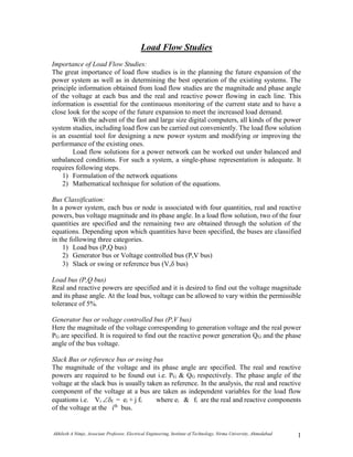
![Akhilesh A Nimje, Associate Professor, Electrical Engineering, Institute of Technology, Nirma University, Ahmedabad 2
Nodal Admittance Matrix (Network Model Formulation)
133112211111312111 )()(
1
yVVyVVyVIIII
nodeAt
)1(][ 13312213121111 yVyVyyyVI
1313121213121111
11
1331221111
;;
1tanarg
yYyYyyyY
busofceadmitingchshunty
YVYVYVI
Similarly, the nodal current equations at bus 2 and bus 3 can be written as follows:
)2(2332222112 YVYVYVI
&
)3(3333223113 YVYVYVI
In Matrix form
)(
3
2
1
333231
232221
131211
3
2
1
A
V
V
V
YYY
YYY
YYY
I
I
I
or in compact form, these equations can be written as
busesthreefortopVYI
q
qpqP
3
1
31,
n
q
qpqp npVYI
busesofnumbernforgeneralIn
1
................3,2,1,
I1 I2
I3
I13
I32
I23
I22
I31
I33
I21I12
I11
1
3
2
y12 = y21
y32 = y23y13 = y31
Three Bus System](data:image/gif;base64,R0lGODlhAQABAIAAAAAAAP///yH5BAEAAAAALAAAAAABAAEAAAIBRAA7)