SlideShare ist ein Scribd-Unternehmen logo
1 von 193
Downloaden Sie, um offline zu lesen
Optoelectronic Devices & Communication Networks
Amplifier
Add/Drop
WDM
Amplifier
WDM
WDM
Switch
Switch
1
2
3
1
n
2
3
n
Montreal
Toronto
Ottawa
Optoelectronic Devices for Communication Networks
» Optical Sources
» LED
» Laser
» Optical Diodes
» WDM
» Fiber Optics
» Optical Amplifiers
» Optical Attenuators
» Optical Isolators
» Optical Switches
» Add/Drop Devices
Optoelectronic Devices for Communication Networks
• Requirements to understand the concepts of
Optoelectronic Devices:
1. We need to study concepts of light properties
2. Some concepts of solid state materials in particular semiconductors.
3. Light + Solid State Materials
Light Properties
• Wave/Particle Duality Nature of Light
• Reflection
• Snell’s Law and Total Internal Reflection (TIR)
• Reflection & Transmission Coefficients
• Fresnel’s Equations
• Intensity, Reflectance and Transmittance
• Refraction
• - Refractive Index
• Interference
• - Multiple Interference and Optical Resonators
• Diffraction
• Fraunhofer Diffraction
• Diffraction Grating
Light Properties
• Dispersion
• Polarization of Light
• Elliptical and Circular Polarization
• Birefringent Optical Devices
• Electro-Optic Effects
• Magneto-Optic Effects
Some Concepts of Solid State Materials
Contents
The Semiconductors in Equilibrium
Nonequilibrium Condition
Generation-Recombination
Generation-Recombination rates
Photoluminescence & Electroluminescence
Photon Absorption
Photon Emission in Semiconductors
Basic Transitions
Radiative
Nonradiative
Spontaneous Emission
Stimulated Emission
Luminescence Efficiency
Internal Quantum Efficiency
External Quantum Efficiency
Photon Absorption
Fresnel Loss
Critical Angle Loss
Energy Band Structures of Semiconductors
PN junctions
Homojunctions, Heterojunctions
Materials
III-V semiconductors
Ternary Semiconductors
Quaternary Semiconductors
II-VI Semiconductors
IV-VI Semiconductors
Light
• The nature of light
Wave/Particle Duality Nature of Light
--Particle nature of light (photon) is used to explain the concepts
of solid state optical sources (LASER, LED), optical detectors,
amplifiers,…
--The wave nature of light is used to explain refraction, diffraction,
polarization,… used to explain the concepts of light transmission in
fiber optics, WDM, add/drop/ modulators,…



h
p
mc
E
c
h
h
E 


 2
The wave nature of Light
• Polarization
• Reflection
• Refraction
• Diffraction
• Interference
To explain these concepts light can be treated as
rays (geometrical optics) or as an electromagnetic
wave (wave optics, studies related to Maxwell
Equations).
An electromagnetic wave consist of two fields:
• Electric Field
• Magnetic Field
Ex
z
Direction of Propagation
By
z
x
y
k
An electromagnetic wave is a travelling wave which has time
varying electric and magnetic fields which are perpendicular to each
other and the direction of propagation,z.
© 1999 S.O. Kasap,Optoelectronics (Prentice Hall)
An electromagnetic wave consist of two components; electrical
field and magnetic field components.
k is the wave vector, and its magnitude is 2π/λ
Light can treated as an EM wave, Ex and By are propagating
through space in such a way that they are always perpendicular to
each other and to the direction of propagation z.
The wave nature of Light
We can treat light as an EM wave with time varying
electric and magnetic fields.
Ex and BY which are propagating through space in such
a way that they are always perpendicular to each
other and to the direction of propagation z.
Traveling wave (sinusoidal):
 
0
0 .
cos
)
,
( 
 

 r
k
t
E
t
r
E
z
Ex
= Eo
sin(t–kz)
Ex
z
Propagation
E
B
k
E and B have constant phase
in this xy plane; a wavefront
E
A plane EM wave travelling along z, has the same Ex (or By) at any point in a
given xy plane. All electric field vectors in a given xy plane are therefore in phase.
The xy planes are of infinite extent in the x and y directions.
© 1999 S.O. Kasap, Optoelectronics (Prentice Hall)
The wave nature of Light y
z
k
Direction of propagation
r
O

E(r,t)
r
A travelling plane EM wave along a direction k
© 1999 S.O. Kasap, Optoelectronics (Prentice Hall)
   
0
0 cos
, 
 

 kr
t
E
t
r
E
t
cons
kz
t tan
0 


 










k
dt
dz
t
z
V 
 2

Phase velocity:
]
Re[
)
,
( )
(
0
0 kz
t
j
j
x e
e
E
t
z
E 
 

During a time interval Δt, a constant phase moves a distance Δz,



z
z
k





2
Phase difference:
k
Wave fronts
r
E
k
Wave fronts
(constant phase surfaces)
z



Wave fronts
P
O
P
A perfect spherical wave
A perfect plane wave A divergent beam
(a) (b) (c)
Examples of possible EM waves
© 1999 S.O. Kasap, Optoelectronics (Prentice Hall)
 
kr
t
r
A
E 
 
cos Spherical wave
   
0
0 cos
, 
 

 kr
t
E
t
r
E Plane wave
t
E
E 2
2
2



  Maxwell’s Wave Equations
Electric field component of
EM wave:
These are the solutions of Maxwell’s equation
Optical Divergence
y
x
Wave fronts
z Beam axis
r
Intensity
(a)
(b)
(c)
2wo

O
Gaussian
2w
(a) Wavefronts of a Gaussian light beam. (b) Light intensity across beam cross
section. (c) Light irradiance (intensity) vs. radial distancer from beam axis (z).
© 1999 S.O. Kasap, Optoelectronics (Prentice Hall)
Wo is called waist radius and 2Wo is called spot size
)
2
(
4
2
0
w


  Is called beam divergence
Gaussian Beams
Refractive Index
c
V 

0
0
1


0
1


V 0


 r

r
v
c
n 


Phase velocity
Speed of light
k(medium) = nk
λ(medium)= λ/n
Isotropic and anisotropic materials?; Optically isotropic/anisotropic?
n and εr are both depend on
The frequency of light (EM wave)
If the light is traveling in dielectric medium, assuming nonmagnetic
and isotropic we can use Maxwell’s equations to solve for electric
field propagation, however we need to define a new phase velocity.
What is εr ??


 + 
 – 
k
Emax
Emax
Wave packet
Two slightly different wavelength waves travelling in the same
direction result in a wave packet that has an amplitude variation
which travels at the group velocity.
© 1999 S.O. Kasap, Optoelectronics (Prentice Hall)
dz/dt = δω/δk or Vg = dω/dk group velocity
Refractive index n and the group index Ng of pure
SiO2 (silica) glass as a function of wavelength.
Ng
n
500 700 900 1100 1300 1500 1700 1900
1.44
1.45
1.46
1.47
1.48
1.49
Wavelength (nm)
© 1999 S.O. Kasap, Optoelectronics (Prentice Hall)
g
g
N
c
d
dn
n
c
dk
d
medium
v 






)
(
What is dispersion?; dispersive
medium?


















2
)
(
n
c
vk
In vacuum group velocity
Is the same as phase velocity.
z
Propagation direction
E
B
k
Area A
vt
A plane EM wave travelling along k crosses an areaA at right angles to the
direction of propagation. In timet, the energy in the cylindrical volume Avt
(shown dashed) flows throughA .
© 1999 S.O. Kasap, Optoelectronics (Prentice Hall)
In EM wave a magnetic field is always accompanying electric field,
Faraday’s Law. In an isotropic dielectric medium Ex = vBy = c/n (By),
where v is the phase velocity and n is index of refraction of the
medium.
n
y
n2 n1
Cladding
Core z
y
r

Fiber axis
The step index optical fiber. The central region, the core, has greater refractive
index than the outer region, the cladding. The fiber has cylindrical symmetry. We
use the coordinates r, , z to represent any point in the fiber. Cladding is
normally much thicker than shown.
© 1999 S.O. Kasap, Optoelectronics (Prentice Hall)
Structure of Fiber Optics
n2
n2
z
2a
y
A
1
2 1
B



A
B
C
 
k1
E
x
n1
Two arbitrary waves 1 and 2 that are initially in phase must remain in phase
after reflections. Otherwise the two will interfere destructively and cancel each
other.
© 1999 S.O. Kasap, Optoelectronics (Prentice Hall)
n2
z
a
y
A
1
2


A
C
k
E
x
y
ay
Guide center

Interference of waves such as 1 and 2 leads to a standing wave pattern along the
y-
direction which propagates alongz.
© 1999 S.O. Kasap,Optoelectronics (Prentice Hall)
n2
Light
n2
n1
y
E(y)
E(y,z,t) = E(y)cos(t – 0z)
m = 0
Field of evanescent wave
(exponential decay)
Field of guided wave
The electric field pattern of the lowest mode traveling wave along the
guide. This mode has m = 0 and the lowest. It is often referred to as the
glazing incidence ray. It has the highest phase velocity along the guide.
© 1999 S.O. Kasap, Optoelectronics (Prentice Hall)
   
z
t
y
E
t
z
y
E m
m 
 
 cos
)
(
2
,
,
1
  















 m
m
m
m
m y
k
z
t
y
k
E
t
z
y
E 



2
1
cos
2
1
cos
2
,
, 0
1
y
E(y)
m = 0 m = 1 m = 2
Cladding
Cladding
Core 2a
n1
n2
n2
The electric field patterns of the first three modes (m = 0, 1, 2)
traveling wave along the guide. Notice different extents of field
penetration into the cladding.
© 1999 S.O. Kasap, Optoelectronics (Prentice Hall)
Low order mode
High order mode
Cladding
Core
Light pulse
t
0 t
Spread, 
Broadened
light pulse
Intensity
Intensity
Axial
Schematic illustration of light propagation in a slab dielectric waveguide. Light pulse
entering the waveguide breaks up into various modes which then propagate at different
group velocities down the guide. At the end of the guide, the modes combine to
constitute the output light pulse which is broader than the input light pulse.
© 1999 S.O. Kasap ,Optoelectronics (Prentice Hall)
n2
z
y
O
i
n1
Ai
 
r
i
Incident Light Bi
Ar
Br
t t
t
RefractedLight
Reflected Light
kt
At
Bt
B
A
B
A
A
r
ki
kr
A light wave travelling in a mediumwith a greater refractive index ( n1 > n2) suffers
reflection and refraction at the boundary.
© 1999 S.O. Kasap,Optoelectronics (Prentice Hall)
Snell’s Law and Total Internal Reflection (TIR)
1
2
sin
sin
n
n
V
V
t
i
t
i




1
1
sin
sin
n
n
V
V
r
i
r
i




Vi = Vr , therefore θi = θr
When θt reaches 90 degree, θi = θc called critical angle
1
2
sin
n
n
c 
 , We have total internal reflection (TIR)
n2
i
n1
> n2
i
Incident
light
t
Transmitted
(refracted) light
Reflected
light
kt
i>c
c
TIR
c
Evanescent wave
ki kr
(a) (b) (c)
Light wave travelling in a more dense mediumstrikes a less dense medium. Depending on
the incidence angle with respect to c, which is determined by the ratio of the refractive
indices, the wave may be transmitted (refracted) or reflected. (a) i < c (b) i = c (c) i
> c and total internal reflection (TIR).
© 1999 S.O. Kasap,Optoelectronics (Prentice Hall)
0
0
1


r
v 
r
v
c
n 


Isotropic and
anisotropic materials
   
z
k
t
j
E
e
z
y
x
E iz
i
y
t 
 
 

exp
,
, 0
,
2
2
1
2
2
2
1
2
2 1
sin
2

















 i
n
n
n




α2 is the attenuation coefficient and 1/ α2 is called penetration depth
x
y
z
Ey
Ex
yEy
^
xEx
^
(a) (b) (c)
E
Plane of polarization
x
^
y
^
E
(a) A linearly polarized wave has its electric field oscillations defined along a line
perpendicular to the direction of propagation,
z. The field vectorE and z define a plane of
polarization
. (b) The E-field oscillations are contained in the plane of polarization. (c) A
linearly polarized light at any instant can be represented by the superposition of two fields
Ex
and Ey with the right magnitude and phase.
E
© 1999 S.O. Kasap,Optoelectronics (Prentice Hall)
ki
n2
n1 > n2
t=90°
Evanescent wave
Reflected
wave
Incident
wave
i r
Er,//
Er,
Ei,
Ei,//
Et,
(b) i > c then the incident wave
suffers total internal reflection.
However, there is an evanescent
wave at the surface of the medium.
z
y
x into paper
i r
Incident
wave
t
Transmitted wave
Ei,//
Ei,
Er,//
Et,
Et,
Er,
Reflected
wave
kt
kr
Light wave travelling in a more dense medium strikes a less dense medium. The plane of
incidence is the plane of the paper and is perpendicular to the flat interface between the
two media. The electric field is normal to the direction of propagation . It can be resolved
into perpendicular (
) and parallel (//) components
(a) i < c then some of the wave
is transmitted into the less dense
medium. Some of the wave is
reflected.
Ei,
© 1999 S.O. Kasap,Optoelectronics(Prentice Hall)
Transverse electric field (TE)
Transverse magnetic Field (TM)
)
.
(
0



 r
k
t
j
i
i
i
e
E
E 
)
.
(
0



 r
k
t
j
r
r
r
e
E
E 
)
.
(
0



 r
k
t
j
t
t
t
e
E
E 
   
z
k
t
j
E
e
z
y
x
E iz
i
y
t 
 
 

exp
,
, 0
,
2
Fresnel’s Equations:
using Snell’s law, and applying boundary conditions:
 
 2
1
2
2
2
1
2
2
,
0
,
0
sin
cos
sin
cos
i
i
i
i
i
r
n
n
E
E
r













 2
1
2
2
,
0
,
0
sin
cos
cos
2
i
i
i
i
t
n
E
E
t










 
  i
i
i
i
i
r
n
n
n
n
E
E
r




cos
sin
cos
sin
2
2
1
2
2
2
2
1
2
2
//
,
0
//
,
0
//






 2
1
2
2
2
//
,
0
//
,
0
//
sin
cos
cos
2
i
i
i
i
t
n
n
n
E
E
t







n = n2/n1
Internal reflection: (a) Magnitude of the reflection coefficients
r// and r
vs. angle of incidence i for n1 = 1.44 and n2 = 1.00. The critical angle is
44°. (b) The corresponding phase changes // and  vs. incidence angle.
//

(b)
60
120
180
Incidence angle, i
0
0.1
0.2
0.3
0.4
0.5
0.6
0.7
0.8
0.9
1
0 10 20 30 40 50 60 70 80 90
| r// |
| r |
c
p
Incidence angle, i
(a)
Magnitude of reflection coefficients Phase changes in degrees
0 10 20 30 40 50 60 70 80 90
c
p
TIR
0
60
20
80
© 1999 S.O. Kasap,Optoelectronics (Prentice Hall)
Polarization angle
 
i
i n



cos
sin
2
1
tan
2
1
2
2









 
i
i
n
n




cos
sin
2
1
2
1
tan 2
2
1
2
2
//









and
r‖ = r┴ = (n1 – n2)/(n1+ n2)
For incident angle close to zero:
The reflection coefficients r// and r vs. angle
of incidence i for n1 = 1.00 and n2 = 1.44.
-1
-0.8
-0.6
-0.4
-0.2
0
0.2
0.4
0.6
0.8
1
0 10 20 30 40 50 60 70 80 90
p r//
r
Incidence angle, i
External reflection
© 1999 S.O. Kasap, Optoelectronics (Prentice Hall)
2
0
2
1
o
r E
V
I 


2
2
,
0
2
,
0



 
 r
E
E
R
i
r
2
//
2
//
,
0
2
//
,
0
// r
E
E
R
i
r


2
2
1
2
1
// 











 
n
n
n
n
R
R
R
2
1
2
2
,
0
2
,
0
2



 








 t
n
n
E
E
n
T
i
t
2
//
1
2
2
//
,
0
2
//
,
0
2
// t
n
n
E
E
n
T
i
t










 2
2
1
2
1
//
4
n
n
n
n
T
T
T



 
Light intensity
Reflectance
for normal incident
Transmittance
d
Semiconductor of
photovoltaic device
Antireflection
coating
Surface
Illustration of how an antireflection coating reduces the
reflected light intensity
n1 n2 n3
A
B
© 1999 S.O. Kasap, Optoelectronics (Prentice Hall)
n1 n2
A
B
n1 n2
C
Schematic illustration of the principle of the dielectric mirror with many low and high
refractive indexlayers and its reflectance.
Reflectance
 (nm)


330 550 770
1 2 2
1
o
1/4 2/4
© 1999 S.O. Kasap, Optoelectronics (Prentice Hall)
Light
n2
A planar dielectric waveguide has a central rectangular region of
higher refractive index n1 than the surrounding region which has
a refractive index n2. It is assumed that the waveguide is
infinitely wide and the central region is of thickness 2 a. It is
illuminated at one end by a monochromatic light source.
n2
n1 > n2
Light
Light Light
© 1999 S.O. Kasap, Optoelectronics (Prentice Hall)
n2
n2
d = 2a


k1
Light
A
B
C



E

n1
A light ray travelling in the guide must interfere constructively with itself to
propagate successfully. Otherwise destructive interference will destroy the
wave.
© 1999 S.O. Kasap, Optoelectronics (Prentice Hall)
z
y
x
 





m
a
n
m
m 







cos
2
2 1
m
m
m
n
k 



 sin
2
sin 1
1 







m
m
m
n
k
k 


 cos
2
cos 1
1 







ΔΦ (AC) = k1(AB + BC) - 2Φ = m(2π), k1 = kn1 = 2πn1/λ
m=0, 1, 2, …
Waveguide condition
n2
Light
n2
n1
y
E(y)
E(y,z,t) = E(y)cos(t – 0z)
m = 0
Field of evanescent wave
(exponential decay)
Field of guided wave
The electric field pattern of the lowest mode traveling wave along the
guide. This mode has m = 0 and the lowest. It is often referred to as the
glazing incidence ray. It has the highest phase velocity along the guide.
© 1999 S.O. Kasap, Optoelectronics (Prentice Hall)
   
z
t
y
E
t
z
y
E m
m 
 
 cos
)
(
2
,
,
1
  















 m
m
m
m
m y
k
z
t
y
k
E
t
z
y
E 



2
1
cos
2
1
cos
2
,
, 0
1
y
E(y)
m = 0 m = 1 m = 2
Cladding
Cladding
Core 2a
n1
n2
n2
The electric field patterns of the first three modes (m = 0, 1, 2)
traveling wave along the guide. Notice different extents of field
penetration into the cladding.
© 1999 S.O. Kasap, Optoelectronics (Prentice Hall)
Low order mode
High order mode
Cladding
Core
Light pulse
t
0 t
Spread, 
Broadened
light pulse
Intensity
Intensity
Axial
Schematic illustration of light propagation in a slab dielectric waveguide. Light pulse
entering the waveguide breaks up into various modes which then propagate at different
group velocities down the guide. At the end of the guide, the modes combine to
constitute the output light pulse which is broader than the input light pulse.
© 1999 S.O. Kasap ,Optoelectronics (Prentice Hall)
Ey (m) is the field distribution along y axis and constitute a mode of propagation.
m is called mode number. Defines the number of modes traveling along the waveguide. For every value
of m we have an angle θm satisfying the waveguide condition provided to satisfy the TIR as well.
Considering these condition one can show that the number of modes should satisfy:
m = ≤ (2V – Φ)/π
V is called V-number  2
1
2
2
2
1
2
n
n
a
V 



For V ≤ π/2, m= 0, it is the lowest mode of propagation referred to single mode waveguides.
The cut-off wavelength (frequency) is a free space wavelength for v = π/2


E
By
Bz
z
y
O


B
E// Ey
Ez
(b) TM mode
(a) TE mode
B//
x (into paper)
Possible modes can be classified in terms of (a) transelectric field (TE)
and (b) transmagnetic field (TM). Plane of incidence is the paper.
© 1999 S.O. Kasap, Optoelectronics (Prentice Hall)
y
E(y)
Cladding
Cladding
Core
2 > 1
1 > c
2 < 1
1 < cut-off
vg1
y
vg2 > vg1
The electric field of TE0 mode extends more into the
cladding as the wavelength increases. As more of the field
is carried by the cladding, the group velocity increases.
© 1999 S.O. Kasap, Optoelectronics (Prentice Hall)
i
n2
n1
> n2
Incident
light
Reflected
light
r
z
Virtual reflecting plane
Penetration depth, 
z
y
The reflected light beam in total internal reflection appears to have been laterally shifted by
an amount z at the interface.
A
B
© 1999 S.O. Kasap, Optoelectronics (Prentice Hall)
Goos-Hanchen shift
i
n2
n1
> n2
Incident
light
Reflected
light
r
When medium B is thin (thickness d is small), the field penetrates to
the BC interface and gives rise to an attenuated wave in medium C.
The effect is the tunnelling of the incident beam in A through B to C.
z
y
d
n1
A
B
C
© 1999 S.O. Kasap, Optoelectronics (Prentice Hall)
Optical Tunneling
Incident
light
Reflected
light
i > c
TIR
(a)
Glass prism
i > c
FTIR
(b)
n1
n1
n2 n1
B = Low refractive index
transparent film ( n2
)
A
C
A
Reflected
Transmitted
(a) A light incident at the long face of a glass prismsuffers TIR; the prismdeflects the
light.
(b) Two prisms separated by a thin low refractive indexfilmforming a beam-splitter cube.
The incident beamis split into two beams by FTIR.
Incident
light
© 1999 S.O. Kasap, Optoelectronics (Prentice Hall)
n
y
n2 n1
Cladding
Core z
y
r

Fiber axis
The step index optical fiber. The central region, the core, has greater refractive
index than the outer region, the cladding. The fiber has cylindrical symmetry. We
use the coordinates r, , z to represent any point in the fiber. Cladding is
normally much thicker than shown.
© 1999 S.O. Kasap, Optoelectronics (Prentice Hall)
For the step index optical fiber Δ = (n1 – n2)/n1
is called normalized index difference
Fiber axis
1
2
3
4
5
Skew ray
1
3
2
4
5
Fiber axis
1
2
3
Meridional ray
1, 3
2
(a) A meridional
ray always
crosses the fiber
axis.
(b) A skew ray
does not have
to cross the
fiber axis. It
zigzags around
the fiber axis.
Illustration of the difference between a meridional ray and a skew ray.
Numbers represent reflections of the ray.
Along the fiber
Ray path projected
on to a plane normal
to fiber axis
Ray path along the fiber
© 1999 S.O. Kasap, Optoelectronics (Prentice Hall)
E
r
E01
Core
Cladding
The electric field distribution of the fundamental mode
in the transverse plane to the fiber axis z. The light
intensity is greatest at the center of the fiber. Intensity
patterns in LP01, LP11 and LP21 modes.
(a) The electric field
of the fundamental
mode
(b) The intensity in
the fundamental
mode LP01
(c) The intensity
in LP11
(d) The intensity
in LP21
© 1999 S.O. Kasap, Optoelectronics (Prentice Hall)
   
z
t
j
r
E
E lm
lm
LP 

 
 exp
.
LPs (linearly polarized waves)
propagating along the fiber
have either TE or TM type
represented by the propagation
of an electric field distribution
Elm(r,Φ) along z.
ELP is the field of the LP mode and βlm is its propagation
constant along z.
V-number
2
2
V
M 
   2
1
1
2
1
2
2
2
1 2
2
2



 n
n
a
n
n
a
V




  405
.
2
2 2
1
2
2
2
1 


 n
n
a
V
c
off
cut


    2
1
2
2
2
1
1
2
1 2
/
/ n
n
n
n
n
n 




Normalized index difference
For V = 2.405, the fiber is called single mode (only the
fundamental mode propagate along the fiber). For V >
2.405 the number of mode increases according to
approximately
Most SM fibers designed
with 1.5<V<2.4
For weakly guided
fiber Δ=0.01, 0.005,..
0 2 4 6
1 3 5
V
b
1
0
0.8
0.6
0.4
0.2
LP01
LP11
LP21
LP02
2.405
Normalized propagation constant b vs. V-number
for a step index fiber for various LP modes.
© 1999 S.O. Kasap, Optoelectronics (Prentice Hall)
 
2
2
2
1
2
2
2
/
n
n
n
k
b




kn2 <β<kn1 Propagation condition
b changes between 0 and 1
C
l
a
d
d
i
n
g
C
o
r
e
  max
A
B
 < c
A
B
 > c
  max
n0 n1
n2
Lost
Propagates
Maximum acceptance angle
max is that which just gives
total internal reflection at the
core-cladding interface, i.e.
when  = max then  = c.
Rays with  > max (e.g. ray
B) become refracted and
penetrate the cladding and are
eventually lost.
Fiber axis
© 1999 S.O. Kasap, Optoelectronics (Prentice Hall)
 
0
2
1
2
2
2
1
max
sin
n
n
n 


2
/
1
2
2
2
1 )
( n
n
NA 

0
max
sin
n
NA


NA
a
V


2

Example values for n1=1.48, n2=1.47;
very close numbers
Typical values of NA = 0.07…,0.25
Numerical Aperture---Maximum Acceptance Angle
Optical waveguides display 3 types of
dispersion:
These are the main sources of dispersion in
the fibers.
• Material dispersion, different
wavelength of light travel at
different velocities within a given
medium.
Due to the variation of n1 of the core wrt
wavelength of the light.
•Waveguide dispersion, β depends
on the wavelength, so even within
a single mode different
wavelengths will propagate at
slightly different speeds.
Due to the variation of group velocity wrt V-
number

t
Spread, ² 
t
0

Spectrum, ² 
1
2
o
Intensity Intensity Intensity
Cladding
Core
Emitter
Very short
light pulse
vg(2)
vg
(1
)
Input
Output
All excitation sources are inherently non-monochromatic and emit within a
spectrum, ², of wavelengths. Waves in the guide with different free space
wavelengths travel at different group velocities due to the wavelength dependence
of n1. The waves arrive at the end of the fiber at different times and hence result in
a broadened output pulse.
© 1999 S.O. Kasap, Optoelectronics (Prentice Hall)





D
L
• Modal dispersion, in
waveguides with more
than one propagating
mode. Modes travel
with different group
velocities.
Due to the number of modes traveling
along the fiber with different group
velocity and different path.
Low order mode
High order mode
Cladding
Core
Light pulse
t
0 t
Spread, 
Broadened
light pulse
Intensity
Intensity
Axial
Schematic illustration of light propagation in a slab dielectric waveguide. Light pulse
entering the waveguide breaks up into various modes which then propagate at different
group velocities down the guide. At the end of the guide, the modes combine to
constitute the output light pulse which is broader than the input light pulse.
© 1999 S.O. Kasap ,Optoelectronics (Prentice Hall)
0
1.2 1.3 1.4 1.5 1.6
1.1
-30
20
30
10
-20
-10
(m)
Dm
Dm + Dw
Dw
0
Dispersion coefficient (ps km-1 nm-1)
Material dispersion coefficient (Dm) for the core material (taken as
SiO2), waveguide dispersion coefficient (Dw) (a = 4.2 m) and the
total or chromatic dispersion coefficient Dch (= Dm + Dw) as a
function of free space wavelength, 
© 1999 S.O. Kasap, Optoelectronics (Prentice Hall)





m
D
L









 2
2


d
n
d
c
Dm


 


D
L
  2
2
2
2
2
2
984
.
1
cn
a
N
D
g

 





P
D
L


 




p
m D
D
D
L
Material
Dispersion
Coefficient
Waveguide
Dispersion
Coefficient
Dp is called profile
dispersion; group velocity
depends on Δ
Core
z
n1x
// x
n1y
// y
Ey
Ex
Ex
Ey
E
 = Pulse spread
Input light p ulse
Output light pulse
t
t

Intensity
Suppose that the core refractive index has different values along two orthogonal
directions corresponding to electric field oscillation direction (polarizations). We can
take x and y axes along these directions. An input light will travel along the fiber with
Ex
and Ey polarizations having different group velocities and hence arrive at the output at
different times
© 1999 S.O. Kasap,Optoelectronics (Prentice Hall)
Polarization Dispersion
Material and waveguide dispersion coefficients in an
optical fiber with a core SiO2-13.5%GeO2 for a = 2.5
to 4 m.
0
–10
10
20
1.2 1.3 1.4 1.5 1.6
–20
 (m)
Dm
Dw
SiO2-13.5%GeO2
2.5
3.0
3.5
4.0
a (m)
Dispersion coefficient (ps km-1 nm-1)
© 1999 S.O. Kasap, Optoelectronics (Prentice Hall)
e.g.
For λ =1.5, and 2a = 8μm
Dm=10 ps/km.nm and
Dw=-6 ps/km.nm
20
-10
-20
-30
10
1.1 1.2 1.3 1.4 1.5 1.6 1.7
0
30
(m)
Dm
Dw
Dch = Dm + Dw
1
Dispersion coefficient (ps km-1 nm-1)
2
n
r
Thin layer of cladding
with a depressed index
Dispersion flattened fiber example. The material dispersion coefficient ( Dm) for the
core material and waveguide dispersion coefficient (Dw) for the doubly clad fiber
result in a flattened small chromatic dispersion between 1 and 2.
© 1999 S.O. Kasap, Optoelectronics (Prentice Hall)
t
0
Emitter
Very short
light pulses
Input Output
Fiber
Photodetector
Digital signal
Information Information
t
0
~2² 
T
t
Output Intensity
Input Intensity
² 
An optical fiber link for transmitting digital information and the effect of
dispersion in the fiber on the output pulses.
© 1999 S.O. Kasap, Optoelectronics (Prentice Hall)
n1
n2
2
1
3
n
O
n1
2
1
3
n
n2
O
O' O''
n2
(a) Multimode step
index fiber. Ray paths
are different so that
rays arrive at different
times.
(b) Graded index fiber.
Ray paths are different
but so are the velocities
along the paths so that
all the rays arrive at the
same time.
2
3
© 1999 S.O. Kasap, Optoelectronics (Prentice Hall)
0.5P
O'
O
(a)
0.25P
O
(b)
0.23P
O
(c)
Graded index (GRIN) rod lenses of different pitches. (a) PointO is on the rod face
center and the lens focuses the rays onto
O' on to the center of the opposite face. (b)
The rays fromO on the rod face center are collimated out. (c)
O is slightly away from
the rod face and the rays are collimated out.
© 1999 S.O. Kasap, Optoelectronics (Prentice Hall)
z
A solid withions
Light direction
k
Ex
Lattice absorption through a crystal. The field in the wave
oscillates the ions which consequently generate "mechanical"
waves in the crystal; energy is thereby transferred from the wave
to lattice vibrations.
© 1999 S.O. Kasap, Optoelectronics (Prentice Hall)
Sources of Loss and Attenuation in Fibers
Absorption depends on
materials, amount of
materials, wavelength, and
the impurities in the
substances.
It is cumulative and depends
on the amount of materials,
e.g. length of the fiber optics.
d
)
1
( 

α is the absorption per unit length and d
is the distance that light travels
Scattered waves
Incident wave Through wave
A dielectric particle smaller than wavelength
Rayleigh scattering involves the polarization of a small dielectric
particle or a region that is much smaller than the light wavelength.
The field forces dipole oscillations in the particle (by polarizing it)
which leads to the emission of EM waves in "many" directions so
that a portion of the light energy is directed away from the incident
beam.
© 1999 S.O. Kasap, Optoelectronics (Prentice Hall)
Escaping wave
 


c 
Microbending
R
Cladding
Core
Field distribution
Sharp bends change the local waveguide geometry that can lead to waves
escaping. The zigzagging ray suddenly finds itself with an incidence
angle  that gives rise to either a transmitted wave, or to a greater
cladding penetration; the field reaches the outside medium and some light
energy is lost.
© 1999 S.O. Kasap, Optoelectronics (Prentice Hall)
Attenuation in Optical Fiber
)
10
(
)
log(
10
1
10
/
L
in
out
out
in
dB
P
P
P
P
L





G. Keiser (Ref. 1)

 34
.
4

dB
Some Concepts of Solid State Materials
Contents
The Semiconductors in Equilibrium
Nonequilibrium Condition
Generation-Recombination
Generation-Recombination rates
Photoluminescence & Electroluminescence
Photon Absorption
Photon Emission in Semiconductors
Basic Transitions
Radiative
Nonradiative
Spontaneous Emission
Stimulated Emission
Luminescence Efficiency
Internal Quantum Efficiency
External Quantum Efficiency
Photon Absorption
Fresnel Loss
Critical Angle Loss
Energy Band Structures of Semiconductors
PN junctions
Homojunctions, Heterojunctions
Materials
III-V semiconductors
Ternary Semiconductors
Quaternary Semiconductors
II-VI Semiconductors
IV-VI Semiconductors
Classification of Devices
• Combination of Electrics
and Mechanics form
Micro/Nano-Electro-
Mechanical Systems
(MEMS/NEMS)
• Combination of Optics,
Electrics and Mechanics
form Micro/Nano-Opto-
Electro-Mechanical
Systems
(MOEMS/NOEMS)
Optical Electronics
Mechanical
MEMS
MOEMS
Schematic illustration of the the structure of a double heterojunction stripe
contact laser diode
Oxide insulator
Stripe electrode
Substrate
Electrode
Active region where J > Jth.
(Emission region)
p-GaAs (Contacting layer)
n-GaAs (Substrate)
p-GaAs (Active layer)
Current
paths
L
W
Cleaved reflecting surface
Elliptical
laser
beam
p-Alx
Ga1-x
As (Confining layer)
n-Alx
Ga1-x
As (Confining layer) 1
2 3
Cleaved reflecting surface
Substrate
© 1999 S.O. Kasap, Optoelectronics (Prentice Hall)
Solid State Optoelectronic Devices
Optical Sources; Laser,
LED
Switches
Photodiodes
Photodetectors
Solar Cells
Type of Semiconductors
• Simple Semiconductors
• Compound Semiconductors
• Direct Band gap Semiconductors
• Indirect Band gap Semiconductors
Some Properties of Some Important Semiconductors
Compound Eg Gap(eV) Transition λ(nm) Bandgap
Diamond 5.4 230 indirect
ZnS 3.75 331 direct
ZnO 3.3 376 indirect
TiO2 3 413 indirect
CdS 2.5 496 direct
CdSe 1.8 689 direct
CdTe 1.55 800 direct
GaAs 1.5 827 direct
InP 1.4 886 direct
Si 1.2 1033 indirect
AgCl 0.32 3875 indirect
PbS 0.3 4133 direct
AgI 0.28 4429 direct
PbTe 0.25 4960 indirect
Common Planes
• {100} Plane
• {110} Plane
• {111} Plane
a
a
a – Lattice Constant
For Silicon
a = 5.34 A
o
Two Interpenetrating Face-Centered Cubic Lattices
Diamond or Zinc Blend Structure
Energy Band Structure of Semiconductors
Concept of positive charges in solids (holes)
Doped Semiconductors
+5
As
+4
Si
+4
Si
+4
Si
+4
Si
+4
Si
+4
Si
+4
Si
+4
Si
Eg
Ec
Ev
Ef
Ed
Conduction
electron
N - Type
Doped Semiconductors
+3
Al
+4
Si
+4
Si
+4
Si
+4
Si
+4
Si
+4
Si
+4
Si
+4
Si
Eg
Ec
Ev
Ef
Valence
hole
Ea
P-type
The Semiconductors in Equilibrium
• The thermal equilibrium concentration of carriers is
independent of time.
• The random generation-recombination of electrons-holes
occur continuously due to the thermal excitation.
• In direct band-to-band generation-recombination, the
electrons and holes are created-annihilated in pairs:
• Gn0 = Gp0 , Rn0 = Rp0
• -The carriers concentrations are independent of time
therefore:
• Gn0 = Gp0 = Rn0 = Rp0
Nonequilibrium Conditions in Semiconductors
• When current exist in a semiconductor device, the semiconductor is
operating under nonequilibrium conditions. In these conditions excess
electrons in conduction band and excess holes in the valance
band exist, due to the external excitation (thermal, electrical, optical…)
in addition to thermal equilibrium concentrations.
n(t) = no + n(t), p(t) = po + p(t)
• The behavior of the excess carriers in semiconductors (diffusion, drift,
recombination, …) which is the fundamental to the operation of
semiconductors (electronic, optoelectronic, ..) is described by the
ambipolar transport or Continuity equations.
Continuity Equations
t
n
n
g
x
E
n
x
n
E
x
n
D
t
p
p
g
x
E
p
x
p
E
x
p
D
n
n
n
n
p
p
p
p






























)
(
)
(
2
2
2
2
Nonequilibrium Conditions in Semiconductors
Generation-Recombination Rates
• The recombination rate is proportional to electron
and hole concentrations.
is the thermal equilibrium generation rate.
dt
t
n
d
dt
t
n
n
d
t
p
t
n
n
dt
t
dn
i
)
(
))
(
(
)]
(
)
(
[
)
( 0
2 

 




)
(
)
( 0 t
n
n
t
n 

 )
(
)
( 0 t
p
p
t
p 


2
i
n

Generation-Recombination Rates
• Electron and holes are created
and recombined in pairs,
therefore,
• n(t) = p(t) and no and po are
independent of time.
)]
(
)
)[(
(
)]
(
))(
(
(
[
))
(
(
0
0
0
0
2
t
n
p
n
t
n
t
p
p
t
n
n
n
dt
t
n
d
i 













Considering a p-type material under low-injection condition,
)
(
))
(
(
0 t
n
p
dt
t
n
d




 0
0
)
0
(
)
0
(
)
( n
t
t
p
e
n
e
n
t
n 








no = (po)-1 is the minority carrier electrons lifetime, constant for low-injections.
Generation-Recombination Rates
• The recombination rate ( a positive quantity) of excess minority carriers
(electrons-holes) for p-type materials is:
0
'
' )
(
n
p
n
t
n
R
R




Similarly, the recombination rate of excess minority carriers for n-type material is:
0
'
' )
(
p
p
n
t
p
R
R




• where po is the minority carrier holes lifetime.
Generation-Recombination Rates
so,
no = (p)-1 and po = (n)-1
[For high injections which is in the case of LASER and LED
operations, n >> no and p >> po ]
• During recombination process if photons are emitted (usually
in direct bandgap semiconductors), the process is called
radiative (important for the operation of optical devices),
otherwise is called nonradiative recombination (takes place
via surface or bulk defects and traps).
Generation-Recombination Rates
• In any carrier-decay process the total lifetime  can be expressed as
nr
r 


1
1
1


where r and nr are the radiative and nonradiative lifetimes
respectively.
The total recombination rate is given by
Where Rr and Rnr are radiative and nonradiative recombination rates
per unit volume respectively and Rsp is called the spontaneous
recombination rate.
sp
nr
r
total R
R
R
R 


pn Junction
The entire semiconductor is a single-
crystal material:
-- p region doped with acceptor
impurity atoms
--n region doped with donor
atoms
--the n and p region are separated
by the metallurgical junction.
-eNa
eNd
x
B-
h+
p n
M
As+
e-
W
Neutral n-region
Neutral p-region
Space charge region
Metallurgical Junction
(a)
(b)
-xp
xn
(c)
E
E (x)
eVbi
ex)
x
x
0
Eo
M
x
n
x
n
- xp
-xp
(e)
(f)
(d)
 (x)
Hole PE(x)
Electron PE(x)
- the potential barrier :
- keeps the large concentration
of electrons from flowing from
the n region into the p region;
- keeps the large concentration
of holes from flowing from the
p region into the n region;
=> The potential barrier maintains
thermal equilibrium.
- the potential of the n region is positive with
respect to the p region => the Fermi energy in
the n region – lower than the Fermi energy in
the p region;
- the total potential barrier – larger than in the
zero-bias case;
- still essentially no charge flow and hence
essentially no current;
-a positive voltage is applied to the p region
with respect to the n region;
- the Fermi energy level – lower in the p
region than in the n region;
- the total potential barrier – reduced => the
electric field in the depletion region – reduced;
 diffusion of holes from the p region across
the depletion region into the n region;
 diffusion of electrons from the n region
across the depletion region into the p region;
- diffusion of carriers => diffusion currents;








 2
ln
i
d
a
t
bi
n
N
N
V
V
-in thermal equilibrium :
- the n region contains many
more electrons in the
conduction band than the p
region;
- the built-in potential barrier
prevents the large density of
electrons from flowing into the
p region;
- the built-in potential barrier
maintains equilibrium between
the carrier distribution on either
side of the junction;





 

kT
qV
n
n bi
n
p exp
0
0
- the electric field Eapp induced by Va – in
opposite direction to the electric field in
depletion region for the thermal equilibrium;
- the net electric field in the depletion region is
reduced below the equilibrium value;
- majority carrier electrons from the n side ->
injected across the depletion region into the p
region;
- majority carrier holes from the p region ->
injected across the depletion region into the n
region;
- Va applied => injection of carriers across the
depletion regions-> a current is created in the
pn junction;
2
/
1
max
2
/
1
max
2
/
1
2
)
(
2
)
(
2
)
(
2


























































 




d
a
d
a
s
R
bi
R
R
bi
d
a
d
a
s
R
bi
d
a
d
a
R
bi
s
p
n
N
N
N
N
eV
E
V
V
W
V
V
N
N
N
N
V
V
e
E
N
N
N
N
e
V
V
x
x
W



2
1
2

















 



d
a
d
a
bi
s
n
p
N
N
N
N
e
V
x
x
W
 For zero bias
For reverse biased
W
V
E bi
2
max


For reverse
biased
For zero bias
When there is no voltage applied across the pn junction  the
junction is in thermal equilibrium => the Fermi energy level –
constant throughout the entire system.
Fp
Fn
bi
V 






























p
n
n
p
i
d
a
bi
n
n
e
kT
p
p
e
kT
n
N
N
e
kT
V ln
ln 2


























i
d
i
a
Fi
Fn
Fp
Fi
n
p
bi
n
N
e
kT
n
N
e
kT
e
E
E
e
E
E
V ln
ln
/
)
(
/
)
(
dx
x
dE
x
dx
x
d
Equation
s
Poisson
s
)
(
)
(
)
(
'
2
2







p
x

+
_
ρ(C/cm³)
d
eN

a
eN

n
x

E
x =0


x
x
s p
dx
x
x
E )
(
1
)
( 

n
n
s
d
p
p
s
a
x
x
x
x
eN
E
x
x
x
x
eN
E











0
),
(
0
),
(


cm
F
Si
For r
s /
)
10
85
.
8
)(
7
.
11
( 14
0




 


n
d
p
a x
N
x
N 
Charge neutrality:
The peak electric field Is at x = 0
s
p
a
s
n
d
x
eN
x
eN
E






max
n
x

p
x

Emax










n
p
n
p
n
p
s
L
n
qD
L
p
qD
J
0
0













 1
exp
kT
qV
J
J a
s - ideal-diode equation;
The bipolar transistor:
- tree separately doped regions
- two pn junctions;
The width of the base region – small compared to the minority carrier diffusion length;
The emitter – largest doping concentration;
The collector – smallest doping concentration;
- the bipolar semiconductor – not a
symmetrical device;
-the transistor – may contain two n
regions or two p regions -> the
impurity doping concentrations in the
emitter and collector = different;
-- the geometry of the two regions –
can be vastly different;
Electromagnetic Spectrum
• Three basic bands; infrared (wavelengths above 0.7m), visible
(wavelengths between 0.4-0.7m), and ultraviolet light (wavelengths
below 0.4m).
• E = h = hc/  ; c =  (μm) =1.24 /E(eV)
• An emitted light from a semiconductor optical device has a wavelength
proportional to the semiconductor band-gap.
• Longer wavelengths for communication systems; Eg  1m. (lower Fiber
loss).
• Shorter wavelengths for printers, image processing,… Eg > 1m.
• Semiconductor materials used to fabricate optical devices depend on the
wavelengths required for the operating systems.
Photoluminescence & Electroluminescence
• The recombination of excess carries in direct bandgap
semiconductors may result in the emission of photon. This
property is generally referred to as luminescence.
• If the excess electrons and holes are created by photon
absorption, then the photon emission from the recombination
process is called photoluminescence.
• If the excess carries are generated by an electric current, then
the photon emission from the recombination process is called
electroluminescence.
Photoluminescence
Optical Absorption
Consider a two-level energy states of E1 and E2.
Also consider that E1 is populated with N1
electron density, and E2 with N2 electron
density.
E1; N1
E2; N2
Absorption
• dN1 states are raised from E1 to E2 i.e dN1 photons are absorbed.
Electrons are created in conduction band and holes in valence band.
• When photons with an intensity of I (x) are traveling through a
semiconductor, going from x position to x + dx position (in 1-D system),
the energy absorbed by semiconductor per unit of time is given by
I (x)dx, where  is the absorption coefficient; the relative number of
photons absorbed per unit distance (cm-1).
dx
x
I
dx
dx
x
dI
x
I
dx
x
I )
(
.
)
(
)
(
)
( 


 





)
(
)
(
x
I
dx
x
dI





x
e
I
x
I 



 0
)
(
where I(0) = I0
Absorption
• Intensity of the photon flux decreases exponentially with distance.
• The absorption coefficient in semiconductor is strong function of photon
energy and band gap energy.
• The absorption coefficient for h < Eg is very small, so the semiconductor
appears transparent to photons in this energy range.
Photoluminescence
Optical Absorption
• When semiconductors are illuminated with light, the photons
may be absorbed (for Eph = hEg= E2 – E1)or they may
propagate through the semiconductors (for EphEg).
• There is a finite probability that electrons in the lower level
absorb energy from incoming electromagnetic field (light)
with frequency of   (E2 – E1)/h and jump to the upper level.
• B12 is proportionality constant,  = 2 - 1 and  = I is the
photon density in the frequency range of .
1
12
1
)
( N
B
dt
dN
ab




Photon Emission in Semiconductors
• When electrons in semiconductors fall from the conduction band to the
valence band, called recombination process, release their energy in form
of light (photon), and/or heat (lattice vibration, phonon).
• N1 and N2 are the concentrations of occupied states in level 1 (E1) and
level 2 (E2) respectively.
Basic Transitions
Radiative
Intrinsic emission
Energetic carriers
Nonradiative
Impurities and defect center involvement
Auger process
Photon Emission in Semiconductors
Spontaneous Emission
Photon Emission in Semiconductors
Einstein Relationship
These are the two fundamental conditions for lasing.
Wave attenuation
Internal Quantum Efficiency
Materials
• Almost all optoelectronic light source depend upon epitaxial
crystal growth techniques where a thin film (a few microns)
of semiconductor alloys are grown on single-crystal
substrate; the film should have roughly the same crystalline
quality. It is necessary to make strain-free heterojunction
with good-quality substrate. The requirement of minimizing
strain effects arises from a desire to avoid interface states
and to encourage long-term device reliability, and this
imposes a lattice-matching condition on the materials used.
Schematic illustration of the the structure of a double heterojunction stripe
contact laser diode
Oxide insulator
Stripe electrode
Substrate
Electrode
Active region where J > Jth.
(Emission region)
p-GaAs (Contacting layer)
n-GaAs (Substrate)
p-GaAs (Active layer)
Current
paths
L
W
Cleaved reflecting surface
Elliptical
laser
beam
p-Alx
Ga1-x
As (Confining layer)
n-Alx
Ga1-x
As (Confining layer) 1
2 3
Cleaved reflecting surface
Substrate
© 1999 S.O. Kasap, Optoelectronics (Prentice Hall)
Solid State Optoelectronic Devices
Optical Sources; Laser,
LED
Switches
Photodiodes
Photodetectors
Solar Cells
Materials
• The constraints of bandgap and lattice match force that more complex
compound must be chosen. These compounds include ternary
(compounds that containing three elements) and quaternary (consisting
of four elements) semiconductors of the form AxB1-xCyD1-y; variation of x
and y are required by the need to adjust the band-gap energy (or desired
wavelength) and for better lattice matching. Quaternary crystals have
more flexibility in that the band gap can be widely varied while
simultaneously keeping the lattice completely matched to a binary
crystal substrate. The important substrates that are available for the
laser diode technology are GaAs, InP and GaP. A few semiconductors and
their alloys can match with these substrates. GaAs was the first material
to emit laser radiation, and its related to III-V compound alloys, are the
most extensively studied developed.
Materials
III-V semiconductors
• Ternary Semiconductors; Mixture of binary-binary
semiconductors; AxB1-xC; mole fraction, x, changes from 0 to 1
(x will be adjusted for specific required wavelength).
GaxAl1-xAs ; In0.53Ga0.47As; In0.52Al0.48As
- Vegard’s Law: The lattice constant of AxB1-xC varies linearly
from the lattice constant of the semiconductor AC to that of
the semiconductor BC.
- The bandgap energy changes as a quadratic function of x.
- The index of refraction changes as x changes.
• The above parameters cannot vary independently
• Quaternary Semiconductors; AxB1-xCyD1-y
(x and y will be adjusted for specific wavelength and matching
lattices).
GaxIn1-xPyAs1-y ; (AlxGa1-x)yIn1-yP; AlxGa1-xAsySb1-y
2
cx
bx
a
Eg 


Materials
• II-VI Semiconductors
• CdZnSe/ZnSe; visible blue lasers.
Hard to dope p-type impurities at
concentration larger than 21018
cm-3
(due to
self-compensation effect). Densities on this
order are required for laser operation.
Materials
• IV-VI semiconductors
• PbSe; PbS; PbTe
• By changing the proportion of Pb atoms in
these materials semiconductor changes from
n- to p-type.
• Operate around 50 Ko
• PbTe/Pb1-xEuxSeyTe1-y operates at 174 Ko
Materials
Materials
• In the near infrared region, the most important and
certainly the most extensively characterized
semiconductors are GaAs, AlAs and their ternary
derivatives AlxGa1-xAs.
• At longer wavelengths, the materials of importance
are InP and ternary and quaternary semiconductors
lattice matched to InP. The smaller band-gap
materials are useful for application in the long
wavelength range.
Energy Band Structure of Semiconductors
0.2
0.4
0.6
0.8
1
1.2
1.4
1.6
1.8
2
2.2
2.4
2.6
0.54 0.55 0.56 0.57 0.58 0.59 0.6 0.61 0.62
Lattice constant, a (nm)
GaP
GaAs
InAs
InP
Direct bandgap
Indirect bandgap
In0.535Ga0.465As
X
Quaternary alloys
with direct bandgap
In1-xGaxAs
Quaternary alloys
with indirect bandgap
Eg (eV)
Bandgap energy Eg and lattice constant a for various III-V alloys of
GaP, GaAs, InP and InAs. A line represents a ternary alloy formed with
compounds from the end points of the line. Solid lines are for direct
bandgap alloys whereas dashed lines for indirect bandgap alloys.
Regions between lines represent quaternary alloys. The line from X to
InP represents quaternary alloys In1-xGaxAs1-yPy made from
In0.535Ga0.465As and InP which are lattice matched to InP.
© 1999 S.O. Kasap, Optoelectronics (Prentice Hall)
3.6 III-V compound semiconductors in optoelectronics Figure
3Q6 represents the bandgap Eg and the lattice parameter a in the
quarternary III-V alloy system. A line joining two points represents
the changes in Eg and a with composition in a ternary alloy composed
of the compounds at the ends of that line. For example, starting at
GaAs point, Eg = 1.42 eV and a = 0.565 nm, and Eg decreases and a
increases as GaAs is alloyed with InAs and we move along the line
joining GaAs to InAs. Eventually at InAs, Eg = 0.35 eV and a =
0.606 nm. Point X in Figure 3Q6 is composed of InAs and GaAs and
it is the ternary alloy InxGa1-xAs. It has Eg = 0.7 eV and a = 0.587
nm which is the same a as that for InP. InxGa1-xAs at X is therefore
lattice matched to InP and can hence be grown on an InP substrate
without creating defects at the interface.
Further, InxGa1-xAs at X can be alloyed with InP to obtain a quarternary alloy
InxGa1-xAsyP1-y whose properties lie on the line joining X and InP and
therefore all have the same lattice parameter as InP but different bandgap. Layers
of InxGa1-xAsyP1-y with composition between X and InP can be grown
epitaxially on an InP substrate by various techniques such as liquid phase epitaxy
(LPE) or molecular beam expitaxy (MBE) .
The shaded area between the solid lines represents the possible values
of Eg and a for the quarternary III-V alloy system in which the bandgap is direct
and hence suitable for direct recombination.
The compositions of the quarternary alloy lattice matched to InP follow
the line from X to InP.
a Given that the InxGa1-xAs at X is In0.535Ga0.465As show that quarternary
alloys In1-xGaxAsyP1-y are lattice matched to InP when y = 2.15x.
b The bandgap energy Eg, in eV for InxGa1-xAsyP1-y lattice matched to
InP is given by the empirical relation,
Eg (eV) = 1.35 - 0.72y + 0.12 y2
Find the composition of the quarternary alloy suitable for an emitter
operating at 1.55 mm.
Materials
Materials
y = 2.2 x
Basic Semiconductor Luminescent Diode Structures
LEDs (Light Emitting Diode)
• Under forward biased when excess minority carriers diffuse
into the neutral semiconductor regions where they recombine
with majority carriers. If this recombination process is direct
band-to-band process, photons are emitted. The output
photon intensity will be proportional to the ideal diode
diffusion current.
• In GaAs, electroluminescence originated primarily on the p-
side of the junction because the efficiency for electron
injection is higher than that for hole injection.
• The recombination is spontaneous and the spectral outputs
have a relatively wide wavelength bandwidth of between 30 –
40 nm.
•  = hc/Eg = 1.24/ Eg
Photon Emission in Semiconductors
Light output
Insulator (oxide)
p
n+ Epit axial layer
A schematic illustration of typical planar surface emitting LED devices. (a)p-layer
grown epitaxially on an n+ substrate. (b) Firstn+ is epitaxially grown and then p region
is formed by dopant diffusion into the epitaxial layer.
Light output
p
Epit axial layers
(a) (b)
n+
Substrate Substrate
n+
n+
Met al electrode
© 1999 S.O. Kasap,Optoelectronics (Prentice Hall)
Basic Semiconductor Luminescent Diode Structures
2eV
2eV
eVo
Holes in VB
Electrons in CB
1.4eV
No bias
With
forward
bias
Ec
Ev
Ec
Ev
EF
EF
(a)
(b)
(c)
(d)
p
n+ p
Ec
GaAs AlGaAs
AlGaAs
p
p
n+
~ 0.2 m
AlGaAs
AlGaAs
(a) A double
heterostructure diode has
two junctions which are
between two different
bandgap semiconductors
(GaAs and AlGaAs)
(b) A simplified energy
band diagram with
exaggerated features. EF
must be uniform.
(c) Forward biased
simplified energy band
diagram.
(d) Forward biased LED.
Schematic illustration of
photons escaping
reabsorption in the
AlGaAs layer and being
emitted from the device.
© 1999 S.O. Kasap, Optoelectronics (Prentice Hall)
GaAs
Ec
Ev
E1
E1
h = E1 – E1
E
In single quantum well (SQW) lasers electrons are
injected by the forward current into the thin GaAs
layer which serves as the active layer. Population
inversion between E1 and E1 is reached even with a
small forward current which results in stimulated
emissions.
© 1999 S.O. Kasap, Optoelectronics (Prentice Hall)
0.4 0.5 0.6 0.7 0.8 0.9 1.0 1.1 1.2 1.3 1.4 1.5 1.6
Blue
Green
Orange
Yellow
Red

1.7
Infrared
Violet
GaAs
GaAs
0.55
P
0.45
GaAs1-yPy
InP
In
0.14
Ga
0.86
As
In1-xGaxAs1-yPy
AlxGa1-xAs
x = 0.43
GaP(N)
GaSb
Indirect
bandgap
InGaN
SiC(Al)
In
0.7
Ga
0.3
As
0.66
P
0.34
In
0.57
Ga
0.43
As
0.95
P
0.05
Free space wavelength coverage by different LED materials fromthe visible spectrumto the
infrared including wavelengths used in optical communications. Hatched region and dashed
lines are indirect Eg materials.
In0.49AlxGa0.51-xP
© 1999 S.O. Kasap, Optoelectronics (Prentice Hall)
E
Ec
Ev
Carrier concentration
per unit energy
Electrons in CB
Holes in VB
h
1
0
Eg
h
h
h
CB
VB

Relative intensity
1
0




h
Relative intensity
(a) (b) (c) (d)
Eg + kBT
(2.5-3)kBT
1/2kBT
Eg
1 2 3
2kBT
(a) Energy band diagramwith possible recombination paths. (b) Energy distribution of
electrons in the CB and holes in the VB. The highest electron concentration is (1/2)
kBT above
Ec . (c) The relative light intensity as a function of photon energy based on (b). (d) Relative
intensity as a function of wavelength in the output spectrumbased on (b) and (c).
© 1999 S.O. Kasap, Optoelectronics (Prentice Hall)
LED Characteristics
V
2
1
(c)
0 20 40
I (mA)
0
(a)
600 650 700
0
0.5
1.0

Relative
intensity
24 nm

655nm
(b)
0 20 40
I (mA)
0
Relative light intensity
(a) A typical output spectrum (relative intensity vs wavelength) from a red GaAsP LED.
(b) Typical output light power vs. forward current. (c) Typical I-V characteristics of a
red LED. The turn-on voltage is around 1.5V.
© 1999 S.O. Kasap, Optoelectronics (Prentice Hall)
800 900
–40°C
25°C
85°C
0
1
740
Relative spectral output power
840 880
Wavelength (nm)
The output spectrum from AlGaAs LED. Values
normalized to peak emission at 25°C.
© 1999 S.O. Kasap, Optoelectronics (Prentice Hall)
Light output
p
Electrodes
Light
Plastic dome
Electrodes
Domed
semiconductor
pn Junction
(a) (b) (c)
n+
n+
(a) Some light suffers total internal reflection and cannot escape. (b) Internal reflections
can be reduced and hence more light can be collected by shaping the semiconductor into a
dome so that the angles of incidence at the semiconductor-air surface are smaller than the
critical angle. (b) An economic method of allowing more light to escape fromthe LED is
to encapsulate it in a transparent plastic dome.
Substrate
© 1999 S.O. Kasap, Optoelectronics (Prentice Hall)
Electrode
SiO2
(insulator)
Electrode
Fiber (multimode)
Epoxy resin
Etched well
Double heterostructure
Light is coupled from a surface emitting LED
into a multimode fiber using an index matching
epoxy. The fiber is bonded to the LED
structure.
(a)
Fiber
A microlens focuses diverging light from a surface
emitting LED into a multimode optical fiber.
Microlens (Ti2O3:SiO2 glass)
(b)
© 1999 S.O. Kasap, Optoelectronics (Prentice Hall)
Schematic illustration of the the structure of a double heterojunction stripe
contact edge emitting LED
Insulation
Stripe electrode
Substrate
Electrode
Active region (emission region)
p+-InP (Eg = 1.35 eV, Cladding layer)
n+-InP (Eg = 1.35 eV, Cladding/Substrate)
n-InGaAs (Eg = 0.83 eV, Active layer)
Current
paths
L
60-70 m
Light beam
p+-InGaAsP (Eg  1 eV, Confining layer)
n+-InGaAsP (Eg  1 eV, Confining layer) 1
2 3
200-300 m
© 1999 S.O. Kasap, Optoelectronics (Prentice Hall)
Active layer Barrier layer
Ec
Ev
E
A multiple quantum well (MQW) structure.
Electrons are injected by the forward current
into active layers which are quantum wells.
© 1999 S.O. Kasap, Optoelectronics (Prentice Hall)
Multimode fiber
Lens
(a)
ELED
Active layer
Light from an edge emitting LED is coupled into a fiber typically by using a lens or a
GRIN rod lens.
GRIN-rod lens
(b)
Single mode fiber
ELED
© 1999 S.O. Kasap, Optoelectronics (Prentice Hall)
LASERS
• The sensitivity of most photosensitive material is greatly
increased at wave-length < 0.7 m; thus, a laser with a short
wave-length is desired for such applications as printers and
image processing. The sensitivity of the human eye range
between the wavelengths of 0.4 and 0.8m and the highest
sensitivity occur at 0.555m or green so it is important to
develop laser in this spectral regime for visual applications.
• Lasers with wavelength between 0.8 – 1.6 m are used in
optical communication systems.
LASERS
• The semiconductor laser diode is a forward bias p-n junction. The structure
appears to be similar to the LED as far as the electron and holes are concerned,
but it is quite different from the point of view of the photons. Electrons and
holes are injected into an active region by forward biasing the laser diode. At low
injection, these electrons and holes recombine (radiative) via the spontaneous
process to emit photons. However, the laser structure is so designed that at
higher injections the emission process occurs by stimulated emission. As we will
discuss, the stimulated emission process provides spectral purity to the photon
output, provides coherent photons, and offers high-speed performance.
• The exact output spectrum from the laser diode depends both on the nature of
the optical cavity and the optical gain versus wavelength characteristics.
• Lasing radiation is only obtained when optical gain in the medium can overcome
the photon loss from the cavity, which requires the diode current I to exceed a
threshold value Ith and gop>gth
• Laser-quality crystals are obtained only with lattice mismatches <0.01% relative
to the substrate.
A
B
L
M1 M2 m = 1
m = 2
m = 8
Relative intensity

m
m m + 1
m - 1
(a) (b) (c)
R ~ 0.4
R ~ 0.8
1 f
Schematic illustration of the Fabry-Perot optical cavity and its properties. (a) Reflected
waves interfere. (b) Only standing EM waves, modes, of certain wavelengths are allowed
in the cavity. (c) Intensity vs. frequency for various modes. R is mirror reflectance and
lower R means higher loss fromthe cavity.
© 1999 S.O. Kasap, Optoelectronics (Prentice Hall)
L
m 






2

m=1,2,3….
   
KL
R
R
I
Icavity 2
2
0
sin
4
1 


f
m m
L
c
m 
 
 )
2
(
L
c
f
2

 Lowest frequency; m=1
Fabry-Perot Optical Resonator
L 
m
m - 1
Fabry-Perot etalon
Partially reflecting plates
Output light
Input light
Transmitted light
Transmitted light through a Fabry-Perot optical cavity.
© 1999 S.O. Kasap, Optoelectronics (Prentice Hall)
 2
0
max
1 R
I
I


 
   
kL
R
R
R
I
I incident
d
transmitte 2
2
2
sin
4
1
1




R
R
F


1
2
/
1

Finesse measures the
loss in the cavity, F
increases as loss
decreases
It is maximum when kL=mπ
m
f
F



 =ratio of the mode separation to
spectral width
LASER Diode Modes of Threshold Conditions


Lasing Conditions:
Population Inversion
Fabry-Perot cavity
gain (of one or several modes) > optical loss
  z
hv
hv
g
e
I
z
I















)
(
)
0
(
)
(
I – optical field intensity
g – gain coefficient in F.P. cavity
- effective absorption coefficient
Γ – optical field confinement factor. (the
fraction of optical power in the active layer)
In one round trip i.e. z = 2L gain
should be > loss for lasing;
During this round trip only R1 &
R2 fractions of optical radiation
are reflected from the two laser
ends 1 & 2.
2
2
1
2
1











n
n
n
n
R
LASER Diode Modes of Threshold Conditions
From the laser conditions: ,
)
(
)
2
( o
I
L
I  1
2

 L
j
e   
m
L 
 2
2 
)
0
(
)
0
(
)
2
(
_
2
2
1 I
e
R
R
I
L
I
g
L









 
2
1
2
1
_
R
R
e
g
L








 
2
1
_
1
ln
2
R
R
g
L 







 
end
th
R
R
L
g 

 




_
2
1
_
1
ln
2
1
Lasing threshold is the point at
which the optical gain is equal to the
total loss αt
end
t
th
g 

 



_
th
th J
g
g 


M– is constant and depends on the
specific device construction.
Thus the gain
z
j
e
o
E
z
E 

 )
(
)
(
Laser Diode Rate Equations
Rate Equations govern the interaction of photons and electrons in
the active region.
ph
sp
R
Bn
dt
d






 = stimulated emission + spontaneous emission - photon loss


Bn
n
qd
J
dt
dn
sp


 = injection - spontaneous recombination - stimulated emission
(shows variation of electron concentration n).
Variation of photon concentration:
The relationship between optical output and the diode drive current:
d - is the depth of carrier-confinement region
B - is a coefficient (Einstein’s) describing the strength of
the optical absorption and emission interactions,;
Rsp - is rate of spontaneous emission into the lasing mode;
τph
– is the photon lifetime;
τsp
– is the spontaneous recombination lifetime;
J – is the injection current density;
Laser Diode Rate Equations
Solving the above Equations for a steady-state condition yields an
expression for the output power.
0

dt
d
0

dt
dn
Steady-state => and
n must exceed a threshold value nth in order for Φ to increase.
In other words J needs to exceed Jth in steady-state condition, when the number
of photons Φ=0.
sp
th
th n
qd
J

 No stimulating emission
This expression defines the current required to sustain an excess
electron density in the laser when spontaneous emission is the only
decay mechanism.
Laser Diode Rate Equations














0
0
qd
J
n
Bn
R
Bn
sp
th
s
th
ph
s
sp
s
th





Now, under steady-state condition at the lasing threshold:
Фs is the steady-state photon density.
0




qd
J
n
R
sp
th
ph
s
sp



ph
ph
sp
th
ph
sp
s
qd
J
n
R 



 


qd
J
n th
sp
th


  ph
sp
th
ph
s R
J
J
qd


 


# of photon resulting from stimulated emission
Adding these two equations: but
The power from the first term is generally concentrated in one or few modes;
The second term generates many modes, in order of 100 modes.
Laser Diode Rate Equations
To find the optical power P0:
c
nL
t 
 time for photons to cross cavity length L.
s

2
1 - is the part travels to right or left (toward output
face)
R is part of the photons reflected and 1-R
part will escape the facet
   
t
R
hv
volume
P
s









1
2
1
0

 
th
ph
J
J
qn
R
W
hc
P 







 



2
)
1
(
2
0
W is the width of active layer
Laser Characteristics
P0
J
Jth
nth
P0 lasing output power ≡ Фs
Threshold
population
inversion
n
Typical output optical power vs. diode current (
I) characteristics and the corresponding
output spectrum of a laser diode.

Laser

Laser
Optical Power
Optical Power
I
0

LED
Optical Power
Ith
Spontaneous
emission
Stimulated
emission
Optical Power
© 1999 S.O. Kasap, Optoelectronics (Prentice Hall)
Laser Characteristics
Resonant Frequency
m
L 
 2
2  

 /
2 n

m
L
n



2
2
2 






c
nLv
2


nL
m
2

So:
n
L
m
2


This states that the cavity resonates (i.e. a standing wave pattern exists
within it) when an integer number m of λ/2 spans the region between the
mirrors. Depending on the laser structures, any number of freq. can satisfy
1
&
)
0
(
)
2
( 2

  L
j
e
I
L
I 
Thus some lasers are single - & some are multi-modes.
The relationship between gain & freq. can be assumed
to have Gaussian form:
 
2
2
0
2
)
0
(
)
( 





 e
g
g
where λ0 is the wavelength at the center of spectrum;
σ is the spectrum width of gain & maximum g(0) is
proportional to the population inversion.
Remember that inside the
optical cavity for
zero phase difference :
1
2

 L
j
e 
; ;
Laser Characteristics
Spacing between the modes:
m
v
c
Ln
m
2
 L
n
m

2

1
2
1 

 m
v
c
Ln
m
Ln
m
Ln
m
Ln
m
Ln
m
2
2
1
2
2 2
2

 





  1
2
2
1 


  v
c
Ln
v
v
c
Ln
m
m
Ln
c
v
2



v
c  2









c
v
c
v
Ln
Ln
c
c
2
2
2
2









m
Ln
2


or
Laser Characteristics
Internal & External Quantum Efficiency
Quantum Efficiency (QE) = # of photons generated for each EHP
injected into the semiconductor junction  a measure of the efficiency
of the electron-to-photon conversion process.
If photons are counted at the junction region, QE is called internal
QE (int
), which depends on the materials of the active junction and
the neighboring regions. For GaAs int
= 65% to 100%.
If photons are counted outside the semiconductor diode QE is
external QE(ext).
Consider an optical cavity of length L , thickness W and width S. Defining a
threshold gain gth as the optical gain needed to balance the total power loss,
due to various losses in the cavity, and the power transmission through the
mirrors .
Laser Characteristics
Internal & External Quantum Efficiency
The optical intensity due to the gain is equal to:
I = Io exp(2Lgth),
There will be lost due to the absorption and the reflections on both ends
by
R1R2 exp(-2Lα)
So: I = Io exp(2Lgth){ R1R2 exp(-2Lα)} = Io (at threshold). Therefore:
1
)
(
2
2
1 

th
g
L
e
R
R
where R1 and R2 are power reflection coefficients of the mirrors,  is
attenuation constant.
Laser Characteristics
Internal & External Quantum Efficiency
2
1
1
ln
2
1
R
R
L
gth 

g is gain constant of the active
region and is roughly
proportional to current density (g
= J).  is a constant.
 
2
1
1
ln
2
1
)
/
1
(
R
R
L
Jth 
 

By measuring Jth, , L, R1 and R2 one
can calculate  (dependent upon the
materials and the junction structure).
The ratio of the power radiated
through mirrors to the total power
generated by the semiconductor
junction is
total
ra
P
P
R
R
L
R
R
L


2
1
2
1
1
ln
2
1
1
ln
2
1

Laser Characteristics
Internal & External Quantum Efficiency
Therefore ext= int(Pra/Ptotal) which can be determined
experimentally from PI characteristic.
For a given Ia (in PI curve current at point a) the number of
electrons injected into the active area/sec = Ia /q and the number
of photons emitted /second = Pa /h
q
I
h
P
a
a
ext
/
/ 
 
q
I
h
P
b
b
ext
/
/ 
 
I
P
h
q
h
I
I
P
P
q
b
a
b
a
ext









)
(
)
(
i.e. ext is proportional to slope of PI curve in the region of I >
Ith.
th
ext
I
I
P
h
q




If we choose Ib = Ith , Pb0 and
h Eg and h/q = Eg /q gives voltage
across the junction in volts.
Laser Characteristics
Power Efficiency
At dc or low frequency the equivalent circuit to a LASER diode may be
viewed as an ideal diode in series with rs.
Therefore the power efficiency =
p =(optical power output)/ (dc electrical power input)
s
g
p
r
I
q
E
I
P
2
)
/
( 


ext
th
I
I
q
h
P 

)
( 

s
g
g
th
ext
p
r
I
q
E
I
q
E
I
I
2
)
/
(
/
)
(





L
Electrode
Current
GaAs
GaAs
n+
p+
Cleaved surface mirror
Electrode
Active region
(stimulated emission region)
A schematic illustration of a GaAs homojunction laser
diode. The cleaved surfaces act as reflecting mirrors.
L
© 1999 S.O. Kasap, Optoelectronics (Prentice Hall)
Typical output optical power vs. diode current (
I) characteristics and the corresponding
output spectrum of a laser diode.

Laser

Laser
Optical Power
Optical Power
I
0

LED
Optical Power
Ith
Spontaneous
emission
Stimulated
emission
Optical Power
© 1999 S.O. Kasap, Optoelectronics (Prentice Hall)
Refractive
index
Photon
density
Active
region
n ~ 5%
2 eV
Holes in VB
Electrons in CB
AlGaAs
AlGaAs
1.4 eV
Ec
Ev
Ec
Ev
(a)
(b)
p
n p
Ec
(a) A double
heterostructure diode has
two junctions which are
between two different
bandgap semiconductors
(GaAs and AlGaAs).
2 eV
(b) Simplified energy
band diagram under a
large forward bias.
Lasing recombination
takes place in the p-
GaAs layer, the
active layer
(~0.1m)
(c) Higher bandgap
materials have a
lower refractive
index
(d) AlGaAs layers
provide lateral optical
confinement.
(c)
(d)
© 1999 S.O. Kasap, Optoelectronics (Prentice Hall)
GaAs
Schematic illustration of the the structure of a double heterojunction stripe
contact laser diode
Oxide insulator
Stripe electrode
Substrate
Electrode
Active region where J > Jth.
(Emission region)
p-GaAs (Contacting layer)
n-GaAs (Substrate)
p-GaAs (Active layer)
Current
paths
L
W
Cleaved reflecting surface
Elliptical
laser
beam
p-Alx
Ga1-x
As (Confining layer)
n-Alx
Ga1-x
As (Confining layer) 1
2 3
Cleaved reflecting surface
Substrate
© 1999 S.O. Kasap, Optoelectronics (Prentice Hall)
Oxide insulation
n-AlGaAs
p+-AlGaAs (Contacting layer)
n-GaAs (Substrate)
p-GaAs (Active layer)
n-AlGaAs (Confining layer)
p-AlGaAs (Confining layer)
Schematic illustration of the cross sectional structure of a buried
heterostructure laser diode.
Electrode
© 1999 S.O. Kasap, Optoelectronics (Prentice Hall)
Height, H
Width W
Length, L
The laser cavity definitions and the output laser beam
characteristics.
Fabry-Perot cavity
Dielectric mirror
Diffraction
limited laser
beam
© 1999 S.O. Kasap, Optoelectronics (Prentice Hall)
778 780 782
Po = 1 mW
Po = 5 mW
Relative optical power
 (nm)
Po = 3 mW
Output spectra of lasing emission from an index guided LD.
At sufficiently high diode currents corresponding to high
optical power, the operation becomes single mode. (Note:
Relative power scale applies to each spectrum individually and
not between spectra)
© 1999 S.O. Kasap, Optoelectronics (Prentice Hall)
Typical optical power output vs. forward current
for a LED and a laser diode.
Current
0
Light power
Laser diode
LED
100 mA
50 mA
5 mW
10 mW
© 1999 S.O. Kasap, Optoelectronics (Prentice Hall)
Corrugated
dielectric structure
Distributed Bragg
reflector
(a) (b)
A
B

q(B/2n) = 
Active layer
(a) Distributed Bragg reflection (DBR) laser principle. (b) Partially reflected waves
at the corrugations can only constitute a reflected wave when the wavelength
satisfies the Bragg condition. Reflected waves A and B interfere constructive when
q(B/2n) = .
© 1999 S.O. Kasap, Optoelectronics (Prentice Hall)

Active layer
Corrugated grating
Guiding layer
(a)
(a) Distributed feedback (DFB) laser structure. (b) Ideal lasing emission output. (c)
Typical output spectrumfroma DFB laser.
Optical power
 (nm)
0.1 nm
Ideal lasing emission

 B
(b) (c)
© 1999 S.O. Kasap, Optoelectronics (Prentice Hall)
Fiber Bragg grating
Bowei Zhang, Presentation for the
Degree of Master of Applied Science
Department of Electrical
and Computer Engineering
Fiber Bragg grating fabrication
Phase Mask: Direct Imprinting
Bowei Zhang, Presentation for the
Degree of Master of Applied Science
Department of Electrical
and Computer Engineering
0th order
(Suppressed)
Diffraction
m = -1
Diffraction
m = +1
Phase Mask
ΛPM
Ge doped
Fiber
248 nm Laser
Active
layer
L D
(a)
Cleaved-coupled-cavity (C3) laser

Cavity Modes


In L
In D
In both
L and D
(b)
© 1999 S.O. Kasap, Optoelectronics (Prentice Hall)
A quantum well (QW) device. (a) Schematic illustration of a quantum well (QW) structure in which a
thin layer of GaAs is sandwiched between two wider bandgap semiconductors (AlGaAs). (b) The
conduction electrons in the GaAs layer are confined (by ² Ec) in the x-direction to a small length d so
that their energy is quantized. (c) The density of states of a two-dimensional QW. The density of states
is constant at each quantized energy level.
AlGaAs AlGaAs
GaAs
y
z
x
d
Ec
Ev
d
E1
E2
E3
g(E)
Density of states
E
Bulk
QW
n = 1
Eg2
Eg1
E n = 2
² Ec
Bulk
QW
² Ev
(a) (b) (c)
Dy
Dz
© 1999 S.O. Kasap, Optoelectronics (Prentice Hall)
Ec
Ev
E1
E1
h = E1 – E1
E
In single quantum well (SQW) lasers electrons are
injected by the forward current into the thin GaAs
layer which serves as the active layer. Population
inversion between E1 and E1 is reached even with a
small forward current which results in stimulated
emissions.
© 1999 S.O. Kasap, Optoelectronics (Prentice Hall)
Active layer Barrier layer
Ec
Ev
E
A multiple quantum well (MQW) structure.
Electrons are injected by the forward current
into active layers which are quantum wells.
© 1999 S.O. Kasap, Optoelectronics (Prentice Hall)

Weitere ähnliche Inhalte

Ähnlich wie Optoelectronic Devices & Communication Networks Overview

Quantum Nanomagetism (USA, 2011)
Quantum Nanomagetism (USA, 2011)Quantum Nanomagetism (USA, 2011)
Quantum Nanomagetism (USA, 2011)oriolespinal
 
2415_web_Lec_30_EM_Waves.5234524524045040pptx
2415_web_Lec_30_EM_Waves.5234524524045040pptx2415_web_Lec_30_EM_Waves.5234524524045040pptx
2415_web_Lec_30_EM_Waves.5234524524045040pptxvikknaguem
 
Optical properties and hall effect
Optical properties and hall effectOptical properties and hall effect
Optical properties and hall effectutpal sarkar
 
Antenna course sofia_2015_lisi_lesson1_v03
Antenna course sofia_2015_lisi_lesson1_v03Antenna course sofia_2015_lisi_lesson1_v03
Antenna course sofia_2015_lisi_lesson1_v03Marco Lisi
 
Advchemchapt7 101015115641-phpapp02
Advchemchapt7 101015115641-phpapp02Advchemchapt7 101015115641-phpapp02
Advchemchapt7 101015115641-phpapp02Cleophas Rwemera
 
Structure of atom plus one focus area notes
Structure of atom plus one focus area notesStructure of atom plus one focus area notes
Structure of atom plus one focus area notessaranyaHC1
 
X ray diffraction(xrd) principle and use
X ray diffraction(xrd) principle and useX ray diffraction(xrd) principle and use
X ray diffraction(xrd) principle and useSrikumar Swain
 
Apchemunit7 111006100549-phpapp02
Apchemunit7 111006100549-phpapp02Apchemunit7 111006100549-phpapp02
Apchemunit7 111006100549-phpapp02Cleophas Rwemera
 
Chapter2-Structure of Atom 2023.pptx
Chapter2-Structure of Atom 2023.pptxChapter2-Structure of Atom 2023.pptx
Chapter2-Structure of Atom 2023.pptxValarmathiRajendran1
 
4 radio wave propagation over the earth
4 radio wave propagation over the earth4 radio wave propagation over the earth
4 radio wave propagation over the earthSolo Hermelin
 
Crystal structure analysis
Crystal structure analysisCrystal structure analysis
Crystal structure analysiszoelfalia
 
Ch5_plasma in food and agri
Ch5_plasma in food and agriCh5_plasma in food and agri
Ch5_plasma in food and agriSITHUHan3
 

Ähnlich wie Optoelectronic Devices & Communication Networks Overview (20)

Quantum Nanomagetism (USA, 2011)
Quantum Nanomagetism (USA, 2011)Quantum Nanomagetism (USA, 2011)
Quantum Nanomagetism (USA, 2011)
 
2415_web_Lec_30_EM_Waves.5234524524045040pptx
2415_web_Lec_30_EM_Waves.5234524524045040pptx2415_web_Lec_30_EM_Waves.5234524524045040pptx
2415_web_Lec_30_EM_Waves.5234524524045040pptx
 
band Theory.pptx
band Theory.pptxband Theory.pptx
band Theory.pptx
 
Optical properties and hall effect
Optical properties and hall effectOptical properties and hall effect
Optical properties and hall effect
 
Antenna course sofia_2015_lisi_lesson1_v03
Antenna course sofia_2015_lisi_lesson1_v03Antenna course sofia_2015_lisi_lesson1_v03
Antenna course sofia_2015_lisi_lesson1_v03
 
Advchemchapt7 101015115641-phpapp02
Advchemchapt7 101015115641-phpapp02Advchemchapt7 101015115641-phpapp02
Advchemchapt7 101015115641-phpapp02
 
x-rays.pdf
x-rays.pdfx-rays.pdf
x-rays.pdf
 
Structure of atom plus one focus area notes
Structure of atom plus one focus area notesStructure of atom plus one focus area notes
Structure of atom plus one focus area notes
 
Ph 101-1
Ph 101-1Ph 101-1
Ph 101-1
 
X ray diffraction(xrd) principle and use
X ray diffraction(xrd) principle and useX ray diffraction(xrd) principle and use
X ray diffraction(xrd) principle and use
 
Chapter 2b
Chapter 2bChapter 2b
Chapter 2b
 
Apchemunit7 111006100549-phpapp02
Apchemunit7 111006100549-phpapp02Apchemunit7 111006100549-phpapp02
Apchemunit7 111006100549-phpapp02
 
Chapter2-Structure of Atom 2023.pptx
Chapter2-Structure of Atom 2023.pptxChapter2-Structure of Atom 2023.pptx
Chapter2-Structure of Atom 2023.pptx
 
Spectroscopy
SpectroscopySpectroscopy
Spectroscopy
 
4 radio wave propagation over the earth
4 radio wave propagation over the earth4 radio wave propagation over the earth
4 radio wave propagation over the earth
 
Electromagnetic waves
Electromagnetic wavesElectromagnetic waves
Electromagnetic waves
 
Chemistry 11
Chemistry 11Chemistry 11
Chemistry 11
 
Crystal structure analysis
Crystal structure analysisCrystal structure analysis
Crystal structure analysis
 
Ch5_plasma in food and agri
Ch5_plasma in food and agriCh5_plasma in food and agri
Ch5_plasma in food and agri
 
Figotin Bath 2005
Figotin Bath 2005Figotin Bath 2005
Figotin Bath 2005
 

Kürzlich hochgeladen

Solving The Right Triangles PowerPoint 2.ppt
Solving The Right Triangles PowerPoint 2.pptSolving The Right Triangles PowerPoint 2.ppt
Solving The Right Triangles PowerPoint 2.pptJasonTagapanGulla
 
NO1 Certified Black Magic Specialist Expert Amil baba in Uae Dubai Abu Dhabi ...
NO1 Certified Black Magic Specialist Expert Amil baba in Uae Dubai Abu Dhabi ...NO1 Certified Black Magic Specialist Expert Amil baba in Uae Dubai Abu Dhabi ...
NO1 Certified Black Magic Specialist Expert Amil baba in Uae Dubai Abu Dhabi ...Amil Baba Dawood bangali
 
complete construction, environmental and economics information of biomass com...
complete construction, environmental and economics information of biomass com...complete construction, environmental and economics information of biomass com...
complete construction, environmental and economics information of biomass com...asadnawaz62
 
CCS355 Neural Networks & Deep Learning Unit 1 PDF notes with Question bank .pdf
CCS355 Neural Networks & Deep Learning Unit 1 PDF notes with Question bank .pdfCCS355 Neural Networks & Deep Learning Unit 1 PDF notes with Question bank .pdf
CCS355 Neural Networks & Deep Learning Unit 1 PDF notes with Question bank .pdfAsst.prof M.Gokilavani
 
Mine Environment II Lab_MI10448MI__________.pptx
Mine Environment II Lab_MI10448MI__________.pptxMine Environment II Lab_MI10448MI__________.pptx
Mine Environment II Lab_MI10448MI__________.pptxRomil Mishra
 
Transport layer issues and challenges - Guide
Transport layer issues and challenges - GuideTransport layer issues and challenges - Guide
Transport layer issues and challenges - GuideGOPINATHS437943
 
Virtual memory management in Operating System
Virtual memory management in Operating SystemVirtual memory management in Operating System
Virtual memory management in Operating SystemRashmi Bhat
 
Main Memory Management in Operating System
Main Memory Management in Operating SystemMain Memory Management in Operating System
Main Memory Management in Operating SystemRashmi Bhat
 
Class 1 | NFPA 72 | Overview Fire Alarm System
Class 1 | NFPA 72 | Overview Fire Alarm SystemClass 1 | NFPA 72 | Overview Fire Alarm System
Class 1 | NFPA 72 | Overview Fire Alarm Systemirfanmechengr
 
welding defects observed during the welding
welding defects observed during the weldingwelding defects observed during the welding
welding defects observed during the weldingMuhammadUzairLiaqat
 
The SRE Report 2024 - Great Findings for the teams
The SRE Report 2024 - Great Findings for the teamsThe SRE Report 2024 - Great Findings for the teams
The SRE Report 2024 - Great Findings for the teamsDILIPKUMARMONDAL6
 
National Level Hackathon Participation Certificate.pdf
National Level Hackathon Participation Certificate.pdfNational Level Hackathon Participation Certificate.pdf
National Level Hackathon Participation Certificate.pdfRajuKanojiya4
 
Indian Dairy Industry Present Status and.ppt
Indian Dairy Industry Present Status and.pptIndian Dairy Industry Present Status and.ppt
Indian Dairy Industry Present Status and.pptMadan Karki
 
TechTAC® CFD Report Summary: A Comparison of Two Types of Tubing Anchor Catchers
TechTAC® CFD Report Summary: A Comparison of Two Types of Tubing Anchor CatchersTechTAC® CFD Report Summary: A Comparison of Two Types of Tubing Anchor Catchers
TechTAC® CFD Report Summary: A Comparison of Two Types of Tubing Anchor Catcherssdickerson1
 
UNIT III ANALOG ELECTRONICS (BASIC ELECTRONICS)
UNIT III ANALOG ELECTRONICS (BASIC ELECTRONICS)UNIT III ANALOG ELECTRONICS (BASIC ELECTRONICS)
UNIT III ANALOG ELECTRONICS (BASIC ELECTRONICS)Dr SOUNDIRARAJ N
 
Introduction-To-Agricultural-Surveillance-Rover.pptx
Introduction-To-Agricultural-Surveillance-Rover.pptxIntroduction-To-Agricultural-Surveillance-Rover.pptx
Introduction-To-Agricultural-Surveillance-Rover.pptxk795866
 
Call Girls Narol 7397865700 Independent Call Girls
Call Girls Narol 7397865700 Independent Call GirlsCall Girls Narol 7397865700 Independent Call Girls
Call Girls Narol 7397865700 Independent Call Girlsssuser7cb4ff
 
Software and Systems Engineering Standards: Verification and Validation of Sy...
Software and Systems Engineering Standards: Verification and Validation of Sy...Software and Systems Engineering Standards: Verification and Validation of Sy...
Software and Systems Engineering Standards: Verification and Validation of Sy...VICTOR MAESTRE RAMIREZ
 
Research Methodology for Engineering pdf
Research Methodology for Engineering pdfResearch Methodology for Engineering pdf
Research Methodology for Engineering pdfCaalaaAbdulkerim
 

Kürzlich hochgeladen (20)

Solving The Right Triangles PowerPoint 2.ppt
Solving The Right Triangles PowerPoint 2.pptSolving The Right Triangles PowerPoint 2.ppt
Solving The Right Triangles PowerPoint 2.ppt
 
NO1 Certified Black Magic Specialist Expert Amil baba in Uae Dubai Abu Dhabi ...
NO1 Certified Black Magic Specialist Expert Amil baba in Uae Dubai Abu Dhabi ...NO1 Certified Black Magic Specialist Expert Amil baba in Uae Dubai Abu Dhabi ...
NO1 Certified Black Magic Specialist Expert Amil baba in Uae Dubai Abu Dhabi ...
 
complete construction, environmental and economics information of biomass com...
complete construction, environmental and economics information of biomass com...complete construction, environmental and economics information of biomass com...
complete construction, environmental and economics information of biomass com...
 
CCS355 Neural Networks & Deep Learning Unit 1 PDF notes with Question bank .pdf
CCS355 Neural Networks & Deep Learning Unit 1 PDF notes with Question bank .pdfCCS355 Neural Networks & Deep Learning Unit 1 PDF notes with Question bank .pdf
CCS355 Neural Networks & Deep Learning Unit 1 PDF notes with Question bank .pdf
 
Mine Environment II Lab_MI10448MI__________.pptx
Mine Environment II Lab_MI10448MI__________.pptxMine Environment II Lab_MI10448MI__________.pptx
Mine Environment II Lab_MI10448MI__________.pptx
 
Transport layer issues and challenges - Guide
Transport layer issues and challenges - GuideTransport layer issues and challenges - Guide
Transport layer issues and challenges - Guide
 
Virtual memory management in Operating System
Virtual memory management in Operating SystemVirtual memory management in Operating System
Virtual memory management in Operating System
 
Main Memory Management in Operating System
Main Memory Management in Operating SystemMain Memory Management in Operating System
Main Memory Management in Operating System
 
Class 1 | NFPA 72 | Overview Fire Alarm System
Class 1 | NFPA 72 | Overview Fire Alarm SystemClass 1 | NFPA 72 | Overview Fire Alarm System
Class 1 | NFPA 72 | Overview Fire Alarm System
 
welding defects observed during the welding
welding defects observed during the weldingwelding defects observed during the welding
welding defects observed during the welding
 
🔝9953056974🔝!!-YOUNG call girls in Rajendra Nagar Escort rvice Shot 2000 nigh...
🔝9953056974🔝!!-YOUNG call girls in Rajendra Nagar Escort rvice Shot 2000 nigh...🔝9953056974🔝!!-YOUNG call girls in Rajendra Nagar Escort rvice Shot 2000 nigh...
🔝9953056974🔝!!-YOUNG call girls in Rajendra Nagar Escort rvice Shot 2000 nigh...
 
The SRE Report 2024 - Great Findings for the teams
The SRE Report 2024 - Great Findings for the teamsThe SRE Report 2024 - Great Findings for the teams
The SRE Report 2024 - Great Findings for the teams
 
National Level Hackathon Participation Certificate.pdf
National Level Hackathon Participation Certificate.pdfNational Level Hackathon Participation Certificate.pdf
National Level Hackathon Participation Certificate.pdf
 
Indian Dairy Industry Present Status and.ppt
Indian Dairy Industry Present Status and.pptIndian Dairy Industry Present Status and.ppt
Indian Dairy Industry Present Status and.ppt
 
TechTAC® CFD Report Summary: A Comparison of Two Types of Tubing Anchor Catchers
TechTAC® CFD Report Summary: A Comparison of Two Types of Tubing Anchor CatchersTechTAC® CFD Report Summary: A Comparison of Two Types of Tubing Anchor Catchers
TechTAC® CFD Report Summary: A Comparison of Two Types of Tubing Anchor Catchers
 
UNIT III ANALOG ELECTRONICS (BASIC ELECTRONICS)
UNIT III ANALOG ELECTRONICS (BASIC ELECTRONICS)UNIT III ANALOG ELECTRONICS (BASIC ELECTRONICS)
UNIT III ANALOG ELECTRONICS (BASIC ELECTRONICS)
 
Introduction-To-Agricultural-Surveillance-Rover.pptx
Introduction-To-Agricultural-Surveillance-Rover.pptxIntroduction-To-Agricultural-Surveillance-Rover.pptx
Introduction-To-Agricultural-Surveillance-Rover.pptx
 
Call Girls Narol 7397865700 Independent Call Girls
Call Girls Narol 7397865700 Independent Call GirlsCall Girls Narol 7397865700 Independent Call Girls
Call Girls Narol 7397865700 Independent Call Girls
 
Software and Systems Engineering Standards: Verification and Validation of Sy...
Software and Systems Engineering Standards: Verification and Validation of Sy...Software and Systems Engineering Standards: Verification and Validation of Sy...
Software and Systems Engineering Standards: Verification and Validation of Sy...
 
Research Methodology for Engineering pdf
Research Methodology for Engineering pdfResearch Methodology for Engineering pdf
Research Methodology for Engineering pdf
 

Optoelectronic Devices & Communication Networks Overview

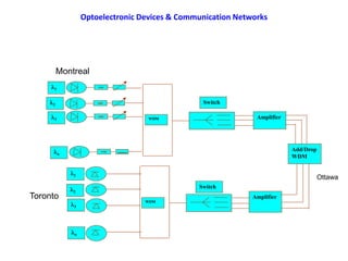
  • 1. Optoelectronic Devices & Communication Networks Amplifier Add/Drop WDM Amplifier WDM WDM Switch Switch 1 2 3 1 n 2 3 n Montreal Toronto Ottawa
  • 2. Optoelectronic Devices for Communication Networks » Optical Sources » LED » Laser » Optical Diodes » WDM » Fiber Optics » Optical Amplifiers » Optical Attenuators » Optical Isolators » Optical Switches » Add/Drop Devices
  • 3. Optoelectronic Devices for Communication Networks • Requirements to understand the concepts of Optoelectronic Devices: 1. We need to study concepts of light properties 2. Some concepts of solid state materials in particular semiconductors. 3. Light + Solid State Materials
  • 4. Light Properties • Wave/Particle Duality Nature of Light • Reflection • Snell’s Law and Total Internal Reflection (TIR) • Reflection & Transmission Coefficients • Fresnel’s Equations • Intensity, Reflectance and Transmittance • Refraction • - Refractive Index • Interference • - Multiple Interference and Optical Resonators • Diffraction • Fraunhofer Diffraction • Diffraction Grating
  • 5. Light Properties • Dispersion • Polarization of Light • Elliptical and Circular Polarization • Birefringent Optical Devices • Electro-Optic Effects • Magneto-Optic Effects
  • 6. Some Concepts of Solid State Materials Contents The Semiconductors in Equilibrium Nonequilibrium Condition Generation-Recombination Generation-Recombination rates Photoluminescence & Electroluminescence Photon Absorption Photon Emission in Semiconductors Basic Transitions Radiative Nonradiative Spontaneous Emission Stimulated Emission Luminescence Efficiency Internal Quantum Efficiency External Quantum Efficiency Photon Absorption Fresnel Loss Critical Angle Loss Energy Band Structures of Semiconductors PN junctions Homojunctions, Heterojunctions Materials III-V semiconductors Ternary Semiconductors Quaternary Semiconductors II-VI Semiconductors IV-VI Semiconductors
  • 7. Light • The nature of light Wave/Particle Duality Nature of Light --Particle nature of light (photon) is used to explain the concepts of solid state optical sources (LASER, LED), optical detectors, amplifiers,… --The wave nature of light is used to explain refraction, diffraction, polarization,… used to explain the concepts of light transmission in fiber optics, WDM, add/drop/ modulators,…    h p mc E c h h E     2
  • 8. The wave nature of Light
  • 9.
  • 10. The wave nature of Light • Polarization • Reflection • Refraction • Diffraction • Interference To explain these concepts light can be treated as rays (geometrical optics) or as an electromagnetic wave (wave optics, studies related to Maxwell Equations). An electromagnetic wave consist of two fields: • Electric Field • Magnetic Field
  • 11. Ex z Direction of Propagation By z x y k An electromagnetic wave is a travelling wave which has time varying electric and magnetic fields which are perpendicular to each other and the direction of propagation,z. © 1999 S.O. Kasap,Optoelectronics (Prentice Hall) An electromagnetic wave consist of two components; electrical field and magnetic field components. k is the wave vector, and its magnitude is 2π/λ Light can treated as an EM wave, Ex and By are propagating through space in such a way that they are always perpendicular to each other and to the direction of propagation z.
  • 12. The wave nature of Light We can treat light as an EM wave with time varying electric and magnetic fields. Ex and BY which are propagating through space in such a way that they are always perpendicular to each other and to the direction of propagation z. Traveling wave (sinusoidal):   0 0 . cos ) , (      r k t E t r E
  • 13. z Ex = Eo sin(t–kz) Ex z Propagation E B k E and B have constant phase in this xy plane; a wavefront E A plane EM wave travelling along z, has the same Ex (or By) at any point in a given xy plane. All electric field vectors in a given xy plane are therefore in phase. The xy planes are of infinite extent in the x and y directions. © 1999 S.O. Kasap, Optoelectronics (Prentice Hall)
  • 14. The wave nature of Light y z k Direction of propagation r O  E(r,t) r A travelling plane EM wave along a direction k © 1999 S.O. Kasap, Optoelectronics (Prentice Hall)     0 0 cos ,      kr t E t r E t cons kz t tan 0                k dt dz t z V   2  Phase velocity: ] Re[ ) , ( ) ( 0 0 kz t j j x e e E t z E     During a time interval Δt, a constant phase moves a distance Δz,    z z k      2 Phase difference:
  • 15. k Wave fronts r E k Wave fronts (constant phase surfaces) z    Wave fronts P O P A perfect spherical wave A perfect plane wave A divergent beam (a) (b) (c) Examples of possible EM waves © 1999 S.O. Kasap, Optoelectronics (Prentice Hall)   kr t r A E    cos Spherical wave     0 0 cos ,      kr t E t r E Plane wave t E E 2 2 2      Maxwell’s Wave Equations Electric field component of EM wave: These are the solutions of Maxwell’s equation Optical Divergence
  • 16. y x Wave fronts z Beam axis r Intensity (a) (b) (c) 2wo  O Gaussian 2w (a) Wavefronts of a Gaussian light beam. (b) Light intensity across beam cross section. (c) Light irradiance (intensity) vs. radial distancer from beam axis (z). © 1999 S.O. Kasap, Optoelectronics (Prentice Hall) Wo is called waist radius and 2Wo is called spot size ) 2 ( 4 2 0 w     Is called beam divergence Gaussian Beams
  • 17. Refractive Index c V   0 0 1   0 1   V 0    r  r v c n    Phase velocity Speed of light k(medium) = nk λ(medium)= λ/n Isotropic and anisotropic materials?; Optically isotropic/anisotropic? n and εr are both depend on The frequency of light (EM wave) If the light is traveling in dielectric medium, assuming nonmagnetic and isotropic we can use Maxwell’s equations to solve for electric field propagation, however we need to define a new phase velocity. What is εr ??
  • 18.    +   –  k Emax Emax Wave packet Two slightly different wavelength waves travelling in the same direction result in a wave packet that has an amplitude variation which travels at the group velocity. © 1999 S.O. Kasap, Optoelectronics (Prentice Hall) dz/dt = δω/δk or Vg = dω/dk group velocity
  • 19. Refractive index n and the group index Ng of pure SiO2 (silica) glass as a function of wavelength. Ng n 500 700 900 1100 1300 1500 1700 1900 1.44 1.45 1.46 1.47 1.48 1.49 Wavelength (nm) © 1999 S.O. Kasap, Optoelectronics (Prentice Hall) g g N c d dn n c dk d medium v        ) ( What is dispersion?; dispersive medium?                   2 ) ( n c vk In vacuum group velocity Is the same as phase velocity.
  • 20. z Propagation direction E B k Area A vt A plane EM wave travelling along k crosses an areaA at right angles to the direction of propagation. In timet, the energy in the cylindrical volume Avt (shown dashed) flows throughA . © 1999 S.O. Kasap, Optoelectronics (Prentice Hall) In EM wave a magnetic field is always accompanying electric field, Faraday’s Law. In an isotropic dielectric medium Ex = vBy = c/n (By), where v is the phase velocity and n is index of refraction of the medium.
  • 21. n y n2 n1 Cladding Core z y r  Fiber axis The step index optical fiber. The central region, the core, has greater refractive index than the outer region, the cladding. The fiber has cylindrical symmetry. We use the coordinates r, , z to represent any point in the fiber. Cladding is normally much thicker than shown. © 1999 S.O. Kasap, Optoelectronics (Prentice Hall) Structure of Fiber Optics
  • 22. n2 n2 z 2a y A 1 2 1 B    A B C   k1 E x n1 Two arbitrary waves 1 and 2 that are initially in phase must remain in phase after reflections. Otherwise the two will interfere destructively and cancel each other. © 1999 S.O. Kasap, Optoelectronics (Prentice Hall)
  • 23. n2 z a y A 1 2   A C k E x y ay Guide center  Interference of waves such as 1 and 2 leads to a standing wave pattern along the y- direction which propagates alongz. © 1999 S.O. Kasap,Optoelectronics (Prentice Hall)
  • 24. n2 Light n2 n1 y E(y) E(y,z,t) = E(y)cos(t – 0z) m = 0 Field of evanescent wave (exponential decay) Field of guided wave The electric field pattern of the lowest mode traveling wave along the guide. This mode has m = 0 and the lowest. It is often referred to as the glazing incidence ray. It has the highest phase velocity along the guide. © 1999 S.O. Kasap, Optoelectronics (Prentice Hall)     z t y E t z y E m m     cos ) ( 2 , , 1                    m m m m m y k z t y k E t z y E     2 1 cos 2 1 cos 2 , , 0 1
  • 25. y E(y) m = 0 m = 1 m = 2 Cladding Cladding Core 2a n1 n2 n2 The electric field patterns of the first three modes (m = 0, 1, 2) traveling wave along the guide. Notice different extents of field penetration into the cladding. © 1999 S.O. Kasap, Optoelectronics (Prentice Hall)
  • 26. Low order mode High order mode Cladding Core Light pulse t 0 t Spread,  Broadened light pulse Intensity Intensity Axial Schematic illustration of light propagation in a slab dielectric waveguide. Light pulse entering the waveguide breaks up into various modes which then propagate at different group velocities down the guide. At the end of the guide, the modes combine to constitute the output light pulse which is broader than the input light pulse. © 1999 S.O. Kasap ,Optoelectronics (Prentice Hall)
  • 27. n2 z y O i n1 Ai   r i Incident Light Bi Ar Br t t t RefractedLight Reflected Light kt At Bt B A B A A r ki kr A light wave travelling in a mediumwith a greater refractive index ( n1 > n2) suffers reflection and refraction at the boundary. © 1999 S.O. Kasap,Optoelectronics (Prentice Hall) Snell’s Law and Total Internal Reflection (TIR) 1 2 sin sin n n V V t i t i     1 1 sin sin n n V V r i r i     Vi = Vr , therefore θi = θr When θt reaches 90 degree, θi = θc called critical angle 1 2 sin n n c   , We have total internal reflection (TIR)
  • 28. n2 i n1 > n2 i Incident light t Transmitted (refracted) light Reflected light kt i>c c TIR c Evanescent wave ki kr (a) (b) (c) Light wave travelling in a more dense mediumstrikes a less dense medium. Depending on the incidence angle with respect to c, which is determined by the ratio of the refractive indices, the wave may be transmitted (refracted) or reflected. (a) i < c (b) i = c (c) i > c and total internal reflection (TIR). © 1999 S.O. Kasap,Optoelectronics (Prentice Hall) 0 0 1   r v  r v c n    Isotropic and anisotropic materials     z k t j E e z y x E iz i y t       exp , , 0 , 2 2 1 2 2 2 1 2 2 1 sin 2                   i n n n     α2 is the attenuation coefficient and 1/ α2 is called penetration depth
  • 29. x y z Ey Ex yEy ^ xEx ^ (a) (b) (c) E Plane of polarization x ^ y ^ E (a) A linearly polarized wave has its electric field oscillations defined along a line perpendicular to the direction of propagation, z. The field vectorE and z define a plane of polarization . (b) The E-field oscillations are contained in the plane of polarization. (c) A linearly polarized light at any instant can be represented by the superposition of two fields Ex and Ey with the right magnitude and phase. E © 1999 S.O. Kasap,Optoelectronics (Prentice Hall)
  • 30. ki n2 n1 > n2 t=90° Evanescent wave Reflected wave Incident wave i r Er,// Er, Ei, Ei,// Et, (b) i > c then the incident wave suffers total internal reflection. However, there is an evanescent wave at the surface of the medium. z y x into paper i r Incident wave t Transmitted wave Ei,// Ei, Er,// Et, Et, Er, Reflected wave kt kr Light wave travelling in a more dense medium strikes a less dense medium. The plane of incidence is the plane of the paper and is perpendicular to the flat interface between the two media. The electric field is normal to the direction of propagation . It can be resolved into perpendicular ( ) and parallel (//) components (a) i < c then some of the wave is transmitted into the less dense medium. Some of the wave is reflected. Ei, © 1999 S.O. Kasap,Optoelectronics(Prentice Hall) Transverse electric field (TE) Transverse magnetic Field (TM) ) . ( 0     r k t j i i i e E E  ) . ( 0     r k t j r r r e E E  ) . ( 0     r k t j t t t e E E      z k t j E e z y x E iz i y t       exp , , 0 , 2
  • 31. Fresnel’s Equations: using Snell’s law, and applying boundary conditions:    2 1 2 2 2 1 2 2 , 0 , 0 sin cos sin cos i i i i i r n n E E r               2 1 2 2 , 0 , 0 sin cos cos 2 i i i i t n E E t               i i i i i r n n n n E E r     cos sin cos sin 2 2 1 2 2 2 2 1 2 2 // , 0 // , 0 //        2 1 2 2 2 // , 0 // , 0 // sin cos cos 2 i i i i t n n n E E t        n = n2/n1
  • 32. Internal reflection: (a) Magnitude of the reflection coefficients r// and r vs. angle of incidence i for n1 = 1.44 and n2 = 1.00. The critical angle is 44°. (b) The corresponding phase changes // and  vs. incidence angle. //  (b) 60 120 180 Incidence angle, i 0 0.1 0.2 0.3 0.4 0.5 0.6 0.7 0.8 0.9 1 0 10 20 30 40 50 60 70 80 90 | r// | | r | c p Incidence angle, i (a) Magnitude of reflection coefficients Phase changes in degrees 0 10 20 30 40 50 60 70 80 90 c p TIR 0 60 20 80 © 1999 S.O. Kasap,Optoelectronics (Prentice Hall) Polarization angle   i i n    cos sin 2 1 tan 2 1 2 2            i i n n     cos sin 2 1 2 1 tan 2 2 1 2 2 //          and r‖ = r┴ = (n1 – n2)/(n1+ n2) For incident angle close to zero:
  • 33. The reflection coefficients r// and r vs. angle of incidence i for n1 = 1.00 and n2 = 1.44. -1 -0.8 -0.6 -0.4 -0.2 0 0.2 0.4 0.6 0.8 1 0 10 20 30 40 50 60 70 80 90 p r// r Incidence angle, i External reflection © 1999 S.O. Kasap, Optoelectronics (Prentice Hall)
  • 34. 2 0 2 1 o r E V I    2 2 , 0 2 , 0       r E E R i r 2 // 2 // , 0 2 // , 0 // r E E R i r   2 2 1 2 1 //               n n n n R R R 2 1 2 2 , 0 2 , 0 2               t n n E E n T i t 2 // 1 2 2 // , 0 2 // , 0 2 // t n n E E n T i t            2 2 1 2 1 // 4 n n n n T T T      Light intensity Reflectance for normal incident Transmittance
  • 35. d Semiconductor of photovoltaic device Antireflection coating Surface Illustration of how an antireflection coating reduces the reflected light intensity n1 n2 n3 A B © 1999 S.O. Kasap, Optoelectronics (Prentice Hall)
  • 36. n1 n2 A B n1 n2 C Schematic illustration of the principle of the dielectric mirror with many low and high refractive indexlayers and its reflectance. Reflectance  (nm)   330 550 770 1 2 2 1 o 1/4 2/4 © 1999 S.O. Kasap, Optoelectronics (Prentice Hall)
  • 37. Light n2 A planar dielectric waveguide has a central rectangular region of higher refractive index n1 than the surrounding region which has a refractive index n2. It is assumed that the waveguide is infinitely wide and the central region is of thickness 2 a. It is illuminated at one end by a monochromatic light source. n2 n1 > n2 Light Light Light © 1999 S.O. Kasap, Optoelectronics (Prentice Hall)
  • 38. n2 n2 d = 2a   k1 Light A B C    E  n1 A light ray travelling in the guide must interfere constructively with itself to propagate successfully. Otherwise destructive interference will destroy the wave. © 1999 S.O. Kasap, Optoelectronics (Prentice Hall) z y x        m a n m m         cos 2 2 1 m m m n k      sin 2 sin 1 1         m m m n k k     cos 2 cos 1 1         ΔΦ (AC) = k1(AB + BC) - 2Φ = m(2π), k1 = kn1 = 2πn1/λ m=0, 1, 2, … Waveguide condition
  • 39. n2 Light n2 n1 y E(y) E(y,z,t) = E(y)cos(t – 0z) m = 0 Field of evanescent wave (exponential decay) Field of guided wave The electric field pattern of the lowest mode traveling wave along the guide. This mode has m = 0 and the lowest. It is often referred to as the glazing incidence ray. It has the highest phase velocity along the guide. © 1999 S.O. Kasap, Optoelectronics (Prentice Hall)     z t y E t z y E m m     cos ) ( 2 , , 1                    m m m m m y k z t y k E t z y E     2 1 cos 2 1 cos 2 , , 0 1
  • 40. y E(y) m = 0 m = 1 m = 2 Cladding Cladding Core 2a n1 n2 n2 The electric field patterns of the first three modes (m = 0, 1, 2) traveling wave along the guide. Notice different extents of field penetration into the cladding. © 1999 S.O. Kasap, Optoelectronics (Prentice Hall)
  • 41. Low order mode High order mode Cladding Core Light pulse t 0 t Spread,  Broadened light pulse Intensity Intensity Axial Schematic illustration of light propagation in a slab dielectric waveguide. Light pulse entering the waveguide breaks up into various modes which then propagate at different group velocities down the guide. At the end of the guide, the modes combine to constitute the output light pulse which is broader than the input light pulse. © 1999 S.O. Kasap ,Optoelectronics (Prentice Hall) Ey (m) is the field distribution along y axis and constitute a mode of propagation. m is called mode number. Defines the number of modes traveling along the waveguide. For every value of m we have an angle θm satisfying the waveguide condition provided to satisfy the TIR as well. Considering these condition one can show that the number of modes should satisfy: m = ≤ (2V – Φ)/π V is called V-number  2 1 2 2 2 1 2 n n a V     For V ≤ π/2, m= 0, it is the lowest mode of propagation referred to single mode waveguides. The cut-off wavelength (frequency) is a free space wavelength for v = π/2
  • 42.   E By Bz z y O   B E// Ey Ez (b) TM mode (a) TE mode B// x (into paper) Possible modes can be classified in terms of (a) transelectric field (TE) and (b) transmagnetic field (TM). Plane of incidence is the paper. © 1999 S.O. Kasap, Optoelectronics (Prentice Hall)
  • 43. y E(y) Cladding Cladding Core 2 > 1 1 > c 2 < 1 1 < cut-off vg1 y vg2 > vg1 The electric field of TE0 mode extends more into the cladding as the wavelength increases. As more of the field is carried by the cladding, the group velocity increases. © 1999 S.O. Kasap, Optoelectronics (Prentice Hall)
  • 44. i n2 n1 > n2 Incident light Reflected light r z Virtual reflecting plane Penetration depth,  z y The reflected light beam in total internal reflection appears to have been laterally shifted by an amount z at the interface. A B © 1999 S.O. Kasap, Optoelectronics (Prentice Hall) Goos-Hanchen shift
  • 45. i n2 n1 > n2 Incident light Reflected light r When medium B is thin (thickness d is small), the field penetrates to the BC interface and gives rise to an attenuated wave in medium C. The effect is the tunnelling of the incident beam in A through B to C. z y d n1 A B C © 1999 S.O. Kasap, Optoelectronics (Prentice Hall) Optical Tunneling
  • 46. Incident light Reflected light i > c TIR (a) Glass prism i > c FTIR (b) n1 n1 n2 n1 B = Low refractive index transparent film ( n2 ) A C A Reflected Transmitted (a) A light incident at the long face of a glass prismsuffers TIR; the prismdeflects the light. (b) Two prisms separated by a thin low refractive indexfilmforming a beam-splitter cube. The incident beamis split into two beams by FTIR. Incident light © 1999 S.O. Kasap, Optoelectronics (Prentice Hall)
  • 47. n y n2 n1 Cladding Core z y r  Fiber axis The step index optical fiber. The central region, the core, has greater refractive index than the outer region, the cladding. The fiber has cylindrical symmetry. We use the coordinates r, , z to represent any point in the fiber. Cladding is normally much thicker than shown. © 1999 S.O. Kasap, Optoelectronics (Prentice Hall) For the step index optical fiber Δ = (n1 – n2)/n1 is called normalized index difference Fiber axis 1 2 3 4 5 Skew ray 1 3 2 4 5 Fiber axis 1 2 3 Meridional ray 1, 3 2 (a) A meridional ray always crosses the fiber axis. (b) A skew ray does not have to cross the fiber axis. It zigzags around the fiber axis. Illustration of the difference between a meridional ray and a skew ray. Numbers represent reflections of the ray. Along the fiber Ray path projected on to a plane normal to fiber axis Ray path along the fiber © 1999 S.O. Kasap, Optoelectronics (Prentice Hall)
  • 48. E r E01 Core Cladding The electric field distribution of the fundamental mode in the transverse plane to the fiber axis z. The light intensity is greatest at the center of the fiber. Intensity patterns in LP01, LP11 and LP21 modes. (a) The electric field of the fundamental mode (b) The intensity in the fundamental mode LP01 (c) The intensity in LP11 (d) The intensity in LP21 © 1999 S.O. Kasap, Optoelectronics (Prentice Hall)     z t j r E E lm lm LP      exp . LPs (linearly polarized waves) propagating along the fiber have either TE or TM type represented by the propagation of an electric field distribution Elm(r,Φ) along z. ELP is the field of the LP mode and βlm is its propagation constant along z.
  • 49. V-number 2 2 V M     2 1 1 2 1 2 2 2 1 2 2 2     n n a n n a V       405 . 2 2 2 1 2 2 2 1     n n a V c off cut       2 1 2 2 2 1 1 2 1 2 / / n n n n n n      Normalized index difference For V = 2.405, the fiber is called single mode (only the fundamental mode propagate along the fiber). For V > 2.405 the number of mode increases according to approximately Most SM fibers designed with 1.5<V<2.4 For weakly guided fiber Δ=0.01, 0.005,..
  • 50. 0 2 4 6 1 3 5 V b 1 0 0.8 0.6 0.4 0.2 LP01 LP11 LP21 LP02 2.405 Normalized propagation constant b vs. V-number for a step index fiber for various LP modes. © 1999 S.O. Kasap, Optoelectronics (Prentice Hall)   2 2 2 1 2 2 2 / n n n k b     kn2 <β<kn1 Propagation condition b changes between 0 and 1
  • 51. C l a d d i n g C o r e   max A B  < c A B  > c   max n0 n1 n2 Lost Propagates Maximum acceptance angle max is that which just gives total internal reflection at the core-cladding interface, i.e. when  = max then  = c. Rays with  > max (e.g. ray B) become refracted and penetrate the cladding and are eventually lost. Fiber axis © 1999 S.O. Kasap, Optoelectronics (Prentice Hall)   0 2 1 2 2 2 1 max sin n n n    2 / 1 2 2 2 1 ) ( n n NA   0 max sin n NA   NA a V   2  Example values for n1=1.48, n2=1.47; very close numbers Typical values of NA = 0.07…,0.25 Numerical Aperture---Maximum Acceptance Angle
  • 52. Optical waveguides display 3 types of dispersion: These are the main sources of dispersion in the fibers. • Material dispersion, different wavelength of light travel at different velocities within a given medium. Due to the variation of n1 of the core wrt wavelength of the light. •Waveguide dispersion, β depends on the wavelength, so even within a single mode different wavelengths will propagate at slightly different speeds. Due to the variation of group velocity wrt V- number  t Spread, ²  t 0  Spectrum, ²  1 2 o Intensity Intensity Intensity Cladding Core Emitter Very short light pulse vg(2) vg (1 ) Input Output All excitation sources are inherently non-monochromatic and emit within a spectrum, ², of wavelengths. Waves in the guide with different free space wavelengths travel at different group velocities due to the wavelength dependence of n1. The waves arrive at the end of the fiber at different times and hence result in a broadened output pulse. © 1999 S.O. Kasap, Optoelectronics (Prentice Hall)      D L
  • 53. • Modal dispersion, in waveguides with more than one propagating mode. Modes travel with different group velocities. Due to the number of modes traveling along the fiber with different group velocity and different path. Low order mode High order mode Cladding Core Light pulse t 0 t Spread,  Broadened light pulse Intensity Intensity Axial Schematic illustration of light propagation in a slab dielectric waveguide. Light pulse entering the waveguide breaks up into various modes which then propagate at different group velocities down the guide. At the end of the guide, the modes combine to constitute the output light pulse which is broader than the input light pulse. © 1999 S.O. Kasap ,Optoelectronics (Prentice Hall)
  • 54. 0 1.2 1.3 1.4 1.5 1.6 1.1 -30 20 30 10 -20 -10 (m) Dm Dm + Dw Dw 0 Dispersion coefficient (ps km-1 nm-1) Material dispersion coefficient (Dm) for the core material (taken as SiO2), waveguide dispersion coefficient (Dw) (a = 4.2 m) and the total or chromatic dispersion coefficient Dch (= Dm + Dw) as a function of free space wavelength,  © 1999 S.O. Kasap, Optoelectronics (Prentice Hall)      m D L           2 2   d n d c Dm       D L   2 2 2 2 2 2 984 . 1 cn a N D g         P D L         p m D D D L Material Dispersion Coefficient Waveguide Dispersion Coefficient Dp is called profile dispersion; group velocity depends on Δ
  • 55. Core z n1x // x n1y // y Ey Ex Ex Ey E  = Pulse spread Input light p ulse Output light pulse t t  Intensity Suppose that the core refractive index has different values along two orthogonal directions corresponding to electric field oscillation direction (polarizations). We can take x and y axes along these directions. An input light will travel along the fiber with Ex and Ey polarizations having different group velocities and hence arrive at the output at different times © 1999 S.O. Kasap,Optoelectronics (Prentice Hall) Polarization Dispersion
  • 56. Material and waveguide dispersion coefficients in an optical fiber with a core SiO2-13.5%GeO2 for a = 2.5 to 4 m. 0 –10 10 20 1.2 1.3 1.4 1.5 1.6 –20  (m) Dm Dw SiO2-13.5%GeO2 2.5 3.0 3.5 4.0 a (m) Dispersion coefficient (ps km-1 nm-1) © 1999 S.O. Kasap, Optoelectronics (Prentice Hall) e.g. For λ =1.5, and 2a = 8μm Dm=10 ps/km.nm and Dw=-6 ps/km.nm
  • 57. 20 -10 -20 -30 10 1.1 1.2 1.3 1.4 1.5 1.6 1.7 0 30 (m) Dm Dw Dch = Dm + Dw 1 Dispersion coefficient (ps km-1 nm-1) 2 n r Thin layer of cladding with a depressed index Dispersion flattened fiber example. The material dispersion coefficient ( Dm) for the core material and waveguide dispersion coefficient (Dw) for the doubly clad fiber result in a flattened small chromatic dispersion between 1 and 2. © 1999 S.O. Kasap, Optoelectronics (Prentice Hall)
  • 58. t 0 Emitter Very short light pulses Input Output Fiber Photodetector Digital signal Information Information t 0 ~2²  T t Output Intensity Input Intensity ²  An optical fiber link for transmitting digital information and the effect of dispersion in the fiber on the output pulses. © 1999 S.O. Kasap, Optoelectronics (Prentice Hall)
  • 59. n1 n2 2 1 3 n O n1 2 1 3 n n2 O O' O'' n2 (a) Multimode step index fiber. Ray paths are different so that rays arrive at different times. (b) Graded index fiber. Ray paths are different but so are the velocities along the paths so that all the rays arrive at the same time. 2 3 © 1999 S.O. Kasap, Optoelectronics (Prentice Hall)
  • 60. 0.5P O' O (a) 0.25P O (b) 0.23P O (c) Graded index (GRIN) rod lenses of different pitches. (a) PointO is on the rod face center and the lens focuses the rays onto O' on to the center of the opposite face. (b) The rays fromO on the rod face center are collimated out. (c) O is slightly away from the rod face and the rays are collimated out. © 1999 S.O. Kasap, Optoelectronics (Prentice Hall)
  • 61. z A solid withions Light direction k Ex Lattice absorption through a crystal. The field in the wave oscillates the ions which consequently generate "mechanical" waves in the crystal; energy is thereby transferred from the wave to lattice vibrations. © 1999 S.O. Kasap, Optoelectronics (Prentice Hall) Sources of Loss and Attenuation in Fibers Absorption depends on materials, amount of materials, wavelength, and the impurities in the substances. It is cumulative and depends on the amount of materials, e.g. length of the fiber optics. d ) 1 (   α is the absorption per unit length and d is the distance that light travels
  • 62. Scattered waves Incident wave Through wave A dielectric particle smaller than wavelength Rayleigh scattering involves the polarization of a small dielectric particle or a region that is much smaller than the light wavelength. The field forces dipole oscillations in the particle (by polarizing it) which leads to the emission of EM waves in "many" directions so that a portion of the light energy is directed away from the incident beam. © 1999 S.O. Kasap, Optoelectronics (Prentice Hall)
  • 63. Escaping wave     c  Microbending R Cladding Core Field distribution Sharp bends change the local waveguide geometry that can lead to waves escaping. The zigzagging ray suddenly finds itself with an incidence angle  that gives rise to either a transmitted wave, or to a greater cladding penetration; the field reaches the outside medium and some light energy is lost. © 1999 S.O. Kasap, Optoelectronics (Prentice Hall)
  • 64. Attenuation in Optical Fiber ) 10 ( ) log( 10 1 10 / L in out out in dB P P P P L      G. Keiser (Ref. 1)   34 . 4  dB
  • 65. Some Concepts of Solid State Materials Contents The Semiconductors in Equilibrium Nonequilibrium Condition Generation-Recombination Generation-Recombination rates Photoluminescence & Electroluminescence Photon Absorption Photon Emission in Semiconductors Basic Transitions Radiative Nonradiative Spontaneous Emission Stimulated Emission Luminescence Efficiency Internal Quantum Efficiency External Quantum Efficiency Photon Absorption Fresnel Loss Critical Angle Loss Energy Band Structures of Semiconductors PN junctions Homojunctions, Heterojunctions Materials III-V semiconductors Ternary Semiconductors Quaternary Semiconductors II-VI Semiconductors IV-VI Semiconductors
  • 66. Classification of Devices • Combination of Electrics and Mechanics form Micro/Nano-Electro- Mechanical Systems (MEMS/NEMS) • Combination of Optics, Electrics and Mechanics form Micro/Nano-Opto- Electro-Mechanical Systems (MOEMS/NOEMS) Optical Electronics Mechanical MEMS MOEMS
  • 67. Schematic illustration of the the structure of a double heterojunction stripe contact laser diode Oxide insulator Stripe electrode Substrate Electrode Active region where J > Jth. (Emission region) p-GaAs (Contacting layer) n-GaAs (Substrate) p-GaAs (Active layer) Current paths L W Cleaved reflecting surface Elliptical laser beam p-Alx Ga1-x As (Confining layer) n-Alx Ga1-x As (Confining layer) 1 2 3 Cleaved reflecting surface Substrate © 1999 S.O. Kasap, Optoelectronics (Prentice Hall) Solid State Optoelectronic Devices Optical Sources; Laser, LED Switches Photodiodes Photodetectors Solar Cells
  • 68. Type of Semiconductors • Simple Semiconductors • Compound Semiconductors • Direct Band gap Semiconductors • Indirect Band gap Semiconductors
  • 69. Some Properties of Some Important Semiconductors Compound Eg Gap(eV) Transition λ(nm) Bandgap Diamond 5.4 230 indirect ZnS 3.75 331 direct ZnO 3.3 376 indirect TiO2 3 413 indirect CdS 2.5 496 direct CdSe 1.8 689 direct CdTe 1.55 800 direct GaAs 1.5 827 direct InP 1.4 886 direct Si 1.2 1033 indirect AgCl 0.32 3875 indirect PbS 0.3 4133 direct AgI 0.28 4429 direct PbTe 0.25 4960 indirect
  • 70. Common Planes • {100} Plane • {110} Plane • {111} Plane a a a – Lattice Constant For Silicon a = 5.34 A o Two Interpenetrating Face-Centered Cubic Lattices Diamond or Zinc Blend Structure
  • 71. Energy Band Structure of Semiconductors
  • 72.
  • 73. Concept of positive charges in solids (holes)
  • 74.
  • 77.
  • 78. The Semiconductors in Equilibrium • The thermal equilibrium concentration of carriers is independent of time. • The random generation-recombination of electrons-holes occur continuously due to the thermal excitation. • In direct band-to-band generation-recombination, the electrons and holes are created-annihilated in pairs: • Gn0 = Gp0 , Rn0 = Rp0 • -The carriers concentrations are independent of time therefore: • Gn0 = Gp0 = Rn0 = Rp0
  • 79. Nonequilibrium Conditions in Semiconductors • When current exist in a semiconductor device, the semiconductor is operating under nonequilibrium conditions. In these conditions excess electrons in conduction band and excess holes in the valance band exist, due to the external excitation (thermal, electrical, optical…) in addition to thermal equilibrium concentrations. n(t) = no + n(t), p(t) = po + p(t) • The behavior of the excess carriers in semiconductors (diffusion, drift, recombination, …) which is the fundamental to the operation of semiconductors (electronic, optoelectronic, ..) is described by the ambipolar transport or Continuity equations.
  • 81. Nonequilibrium Conditions in Semiconductors Generation-Recombination Rates • The recombination rate is proportional to electron and hole concentrations. is the thermal equilibrium generation rate. dt t n d dt t n n d t p t n n dt t dn i ) ( )) ( ( )] ( ) ( [ ) ( 0 2         ) ( ) ( 0 t n n t n    ) ( ) ( 0 t p p t p    2 i n 
  • 82. Generation-Recombination Rates • Electron and holes are created and recombined in pairs, therefore, • n(t) = p(t) and no and po are independent of time. )] ( ) )[( ( )] ( ))( ( ( [ )) ( ( 0 0 0 0 2 t n p n t n t p p t n n n dt t n d i               Considering a p-type material under low-injection condition, ) ( )) ( ( 0 t n p dt t n d      0 0 ) 0 ( ) 0 ( ) ( n t t p e n e n t n          no = (po)-1 is the minority carrier electrons lifetime, constant for low-injections.
  • 83. Generation-Recombination Rates • The recombination rate ( a positive quantity) of excess minority carriers (electrons-holes) for p-type materials is: 0 ' ' ) ( n p n t n R R     Similarly, the recombination rate of excess minority carriers for n-type material is: 0 ' ' ) ( p p n t p R R     • where po is the minority carrier holes lifetime.
  • 84. Generation-Recombination Rates so, no = (p)-1 and po = (n)-1 [For high injections which is in the case of LASER and LED operations, n >> no and p >> po ] • During recombination process if photons are emitted (usually in direct bandgap semiconductors), the process is called radiative (important for the operation of optical devices), otherwise is called nonradiative recombination (takes place via surface or bulk defects and traps).
  • 85. Generation-Recombination Rates • In any carrier-decay process the total lifetime  can be expressed as nr r    1 1 1   where r and nr are the radiative and nonradiative lifetimes respectively. The total recombination rate is given by Where Rr and Rnr are radiative and nonradiative recombination rates per unit volume respectively and Rsp is called the spontaneous recombination rate. sp nr r total R R R R   
  • 86.
  • 87. pn Junction The entire semiconductor is a single- crystal material: -- p region doped with acceptor impurity atoms --n region doped with donor atoms --the n and p region are separated by the metallurgical junction.
  • 88. -eNa eNd x B- h+ p n M As+ e- W Neutral n-region Neutral p-region Space charge region Metallurgical Junction (a) (b) -xp xn (c) E E (x) eVbi ex) x x 0 Eo M x n x n - xp -xp (e) (f) (d)  (x) Hole PE(x) Electron PE(x)
  • 89. - the potential barrier : - keeps the large concentration of electrons from flowing from the n region into the p region; - keeps the large concentration of holes from flowing from the p region into the n region; => The potential barrier maintains thermal equilibrium.
  • 90. - the potential of the n region is positive with respect to the p region => the Fermi energy in the n region – lower than the Fermi energy in the p region; - the total potential barrier – larger than in the zero-bias case; - still essentially no charge flow and hence essentially no current;
  • 91. -a positive voltage is applied to the p region with respect to the n region; - the Fermi energy level – lower in the p region than in the n region; - the total potential barrier – reduced => the electric field in the depletion region – reduced;  diffusion of holes from the p region across the depletion region into the n region;  diffusion of electrons from the n region across the depletion region into the p region; - diffusion of carriers => diffusion currents;
  • 92.          2 ln i d a t bi n N N V V -in thermal equilibrium : - the n region contains many more electrons in the conduction band than the p region; - the built-in potential barrier prevents the large density of electrons from flowing into the p region; - the built-in potential barrier maintains equilibrium between the carrier distribution on either side of the junction;         kT qV n n bi n p exp 0 0
  • 93. - the electric field Eapp induced by Va – in opposite direction to the electric field in depletion region for the thermal equilibrium; - the net electric field in the depletion region is reduced below the equilibrium value; - majority carrier electrons from the n side -> injected across the depletion region into the p region; - majority carrier holes from the p region -> injected across the depletion region into the n region; - Va applied => injection of carriers across the depletion regions-> a current is created in the pn junction;
  • 94.
  • 96. When there is no voltage applied across the pn junction  the junction is in thermal equilibrium => the Fermi energy level – constant throughout the entire system. Fp Fn bi V                                p n n p i d a bi n n e kT p p e kT n N N e kT V ln ln 2                           i d i a Fi Fn Fp Fi n p bi n N e kT n N e kT e E E e E E V ln ln / ) ( / ) (
  • 97. dx x dE x dx x d Equation s Poisson s ) ( ) ( ) ( ' 2 2        p x  + _ ρ(C/cm³) d eN  a eN  n x  E x =0   x x s p dx x x E ) ( 1 ) (   n n s d p p s a x x x x eN E x x x x eN E            0 ), ( 0 ), (   cm F Si For r s / ) 10 85 . 8 )( 7 . 11 ( 14 0         n d p a x N x N  Charge neutrality: The peak electric field Is at x = 0 s p a s n d x eN x eN E       max n x  p x  Emax
  • 99. The bipolar transistor: - tree separately doped regions - two pn junctions; The width of the base region – small compared to the minority carrier diffusion length; The emitter – largest doping concentration; The collector – smallest doping concentration;
  • 100. - the bipolar semiconductor – not a symmetrical device; -the transistor – may contain two n regions or two p regions -> the impurity doping concentrations in the emitter and collector = different; -- the geometry of the two regions – can be vastly different;
  • 101.
  • 102. Electromagnetic Spectrum • Three basic bands; infrared (wavelengths above 0.7m), visible (wavelengths between 0.4-0.7m), and ultraviolet light (wavelengths below 0.4m). • E = h = hc/  ; c =  (μm) =1.24 /E(eV) • An emitted light from a semiconductor optical device has a wavelength proportional to the semiconductor band-gap. • Longer wavelengths for communication systems; Eg  1m. (lower Fiber loss). • Shorter wavelengths for printers, image processing,… Eg > 1m. • Semiconductor materials used to fabricate optical devices depend on the wavelengths required for the operating systems.
  • 103. Photoluminescence & Electroluminescence • The recombination of excess carries in direct bandgap semiconductors may result in the emission of photon. This property is generally referred to as luminescence. • If the excess electrons and holes are created by photon absorption, then the photon emission from the recombination process is called photoluminescence. • If the excess carries are generated by an electric current, then the photon emission from the recombination process is called electroluminescence.
  • 104. Photoluminescence Optical Absorption Consider a two-level energy states of E1 and E2. Also consider that E1 is populated with N1 electron density, and E2 with N2 electron density. E1; N1 E2; N2
  • 105. Absorption • dN1 states are raised from E1 to E2 i.e dN1 photons are absorbed. Electrons are created in conduction band and holes in valence band. • When photons with an intensity of I (x) are traveling through a semiconductor, going from x position to x + dx position (in 1-D system), the energy absorbed by semiconductor per unit of time is given by I (x)dx, where  is the absorption coefficient; the relative number of photons absorbed per unit distance (cm-1). dx x I dx dx x dI x I dx x I ) ( . ) ( ) ( ) (           ) ( ) ( x I dx x dI      x e I x I      0 ) ( where I(0) = I0
  • 106. Absorption • Intensity of the photon flux decreases exponentially with distance. • The absorption coefficient in semiconductor is strong function of photon energy and band gap energy. • The absorption coefficient for h < Eg is very small, so the semiconductor appears transparent to photons in this energy range.
  • 107. Photoluminescence Optical Absorption • When semiconductors are illuminated with light, the photons may be absorbed (for Eph = hEg= E2 – E1)or they may propagate through the semiconductors (for EphEg). • There is a finite probability that electrons in the lower level absorb energy from incoming electromagnetic field (light) with frequency of   (E2 – E1)/h and jump to the upper level. • B12 is proportionality constant,  = 2 - 1 and  = I is the photon density in the frequency range of . 1 12 1 ) ( N B dt dN ab    
  • 108. Photon Emission in Semiconductors • When electrons in semiconductors fall from the conduction band to the valence band, called recombination process, release their energy in form of light (photon), and/or heat (lattice vibration, phonon). • N1 and N2 are the concentrations of occupied states in level 1 (E1) and level 2 (E2) respectively. Basic Transitions Radiative Intrinsic emission Energetic carriers Nonradiative Impurities and defect center involvement Auger process
  • 109. Photon Emission in Semiconductors
  • 110. Photon Emission in Semiconductors
  • 111. Photon Emission in Semiconductors Spontaneous Emission
  • 112. Photon Emission in Semiconductors
  • 113. Photon Emission in Semiconductors
  • 114. Photon Emission in Semiconductors
  • 115.
  • 117. Einstein Relationship These are the two fundamental conditions for lasing.
  • 118.
  • 120.
  • 121.
  • 124.
  • 125.
  • 126.
  • 127. Materials • Almost all optoelectronic light source depend upon epitaxial crystal growth techniques where a thin film (a few microns) of semiconductor alloys are grown on single-crystal substrate; the film should have roughly the same crystalline quality. It is necessary to make strain-free heterojunction with good-quality substrate. The requirement of minimizing strain effects arises from a desire to avoid interface states and to encourage long-term device reliability, and this imposes a lattice-matching condition on the materials used.
  • 128. Schematic illustration of the the structure of a double heterojunction stripe contact laser diode Oxide insulator Stripe electrode Substrate Electrode Active region where J > Jth. (Emission region) p-GaAs (Contacting layer) n-GaAs (Substrate) p-GaAs (Active layer) Current paths L W Cleaved reflecting surface Elliptical laser beam p-Alx Ga1-x As (Confining layer) n-Alx Ga1-x As (Confining layer) 1 2 3 Cleaved reflecting surface Substrate © 1999 S.O. Kasap, Optoelectronics (Prentice Hall) Solid State Optoelectronic Devices Optical Sources; Laser, LED Switches Photodiodes Photodetectors Solar Cells
  • 129. Materials • The constraints of bandgap and lattice match force that more complex compound must be chosen. These compounds include ternary (compounds that containing three elements) and quaternary (consisting of four elements) semiconductors of the form AxB1-xCyD1-y; variation of x and y are required by the need to adjust the band-gap energy (or desired wavelength) and for better lattice matching. Quaternary crystals have more flexibility in that the band gap can be widely varied while simultaneously keeping the lattice completely matched to a binary crystal substrate. The important substrates that are available for the laser diode technology are GaAs, InP and GaP. A few semiconductors and their alloys can match with these substrates. GaAs was the first material to emit laser radiation, and its related to III-V compound alloys, are the most extensively studied developed.
  • 130. Materials III-V semiconductors • Ternary Semiconductors; Mixture of binary-binary semiconductors; AxB1-xC; mole fraction, x, changes from 0 to 1 (x will be adjusted for specific required wavelength). GaxAl1-xAs ; In0.53Ga0.47As; In0.52Al0.48As - Vegard’s Law: The lattice constant of AxB1-xC varies linearly from the lattice constant of the semiconductor AC to that of the semiconductor BC. - The bandgap energy changes as a quadratic function of x. - The index of refraction changes as x changes. • The above parameters cannot vary independently • Quaternary Semiconductors; AxB1-xCyD1-y (x and y will be adjusted for specific wavelength and matching lattices). GaxIn1-xPyAs1-y ; (AlxGa1-x)yIn1-yP; AlxGa1-xAsySb1-y 2 cx bx a Eg   
  • 131. Materials • II-VI Semiconductors • CdZnSe/ZnSe; visible blue lasers. Hard to dope p-type impurities at concentration larger than 21018 cm-3 (due to self-compensation effect). Densities on this order are required for laser operation.
  • 132. Materials • IV-VI semiconductors • PbSe; PbS; PbTe • By changing the proportion of Pb atoms in these materials semiconductor changes from n- to p-type. • Operate around 50 Ko • PbTe/Pb1-xEuxSeyTe1-y operates at 174 Ko
  • 134. Materials • In the near infrared region, the most important and certainly the most extensively characterized semiconductors are GaAs, AlAs and their ternary derivatives AlxGa1-xAs. • At longer wavelengths, the materials of importance are InP and ternary and quaternary semiconductors lattice matched to InP. The smaller band-gap materials are useful for application in the long wavelength range.
  • 135. Energy Band Structure of Semiconductors
  • 136. 0.2 0.4 0.6 0.8 1 1.2 1.4 1.6 1.8 2 2.2 2.4 2.6 0.54 0.55 0.56 0.57 0.58 0.59 0.6 0.61 0.62 Lattice constant, a (nm) GaP GaAs InAs InP Direct bandgap Indirect bandgap In0.535Ga0.465As X Quaternary alloys with direct bandgap In1-xGaxAs Quaternary alloys with indirect bandgap Eg (eV) Bandgap energy Eg and lattice constant a for various III-V alloys of GaP, GaAs, InP and InAs. A line represents a ternary alloy formed with compounds from the end points of the line. Solid lines are for direct bandgap alloys whereas dashed lines for indirect bandgap alloys. Regions between lines represent quaternary alloys. The line from X to InP represents quaternary alloys In1-xGaxAs1-yPy made from In0.535Ga0.465As and InP which are lattice matched to InP. © 1999 S.O. Kasap, Optoelectronics (Prentice Hall)
  • 137. 3.6 III-V compound semiconductors in optoelectronics Figure 3Q6 represents the bandgap Eg and the lattice parameter a in the quarternary III-V alloy system. A line joining two points represents the changes in Eg and a with composition in a ternary alloy composed of the compounds at the ends of that line. For example, starting at GaAs point, Eg = 1.42 eV and a = 0.565 nm, and Eg decreases and a increases as GaAs is alloyed with InAs and we move along the line joining GaAs to InAs. Eventually at InAs, Eg = 0.35 eV and a = 0.606 nm. Point X in Figure 3Q6 is composed of InAs and GaAs and it is the ternary alloy InxGa1-xAs. It has Eg = 0.7 eV and a = 0.587 nm which is the same a as that for InP. InxGa1-xAs at X is therefore lattice matched to InP and can hence be grown on an InP substrate without creating defects at the interface.
  • 138. Further, InxGa1-xAs at X can be alloyed with InP to obtain a quarternary alloy InxGa1-xAsyP1-y whose properties lie on the line joining X and InP and therefore all have the same lattice parameter as InP but different bandgap. Layers of InxGa1-xAsyP1-y with composition between X and InP can be grown epitaxially on an InP substrate by various techniques such as liquid phase epitaxy (LPE) or molecular beam expitaxy (MBE) . The shaded area between the solid lines represents the possible values of Eg and a for the quarternary III-V alloy system in which the bandgap is direct and hence suitable for direct recombination. The compositions of the quarternary alloy lattice matched to InP follow the line from X to InP. a Given that the InxGa1-xAs at X is In0.535Ga0.465As show that quarternary alloys In1-xGaxAsyP1-y are lattice matched to InP when y = 2.15x. b The bandgap energy Eg, in eV for InxGa1-xAsyP1-y lattice matched to InP is given by the empirical relation, Eg (eV) = 1.35 - 0.72y + 0.12 y2 Find the composition of the quarternary alloy suitable for an emitter operating at 1.55 mm.
  • 141. Basic Semiconductor Luminescent Diode Structures LEDs (Light Emitting Diode) • Under forward biased when excess minority carriers diffuse into the neutral semiconductor regions where they recombine with majority carriers. If this recombination process is direct band-to-band process, photons are emitted. The output photon intensity will be proportional to the ideal diode diffusion current. • In GaAs, electroluminescence originated primarily on the p- side of the junction because the efficiency for electron injection is higher than that for hole injection. • The recombination is spontaneous and the spectral outputs have a relatively wide wavelength bandwidth of between 30 – 40 nm. •  = hc/Eg = 1.24/ Eg
  • 142. Photon Emission in Semiconductors
  • 143. Light output Insulator (oxide) p n+ Epit axial layer A schematic illustration of typical planar surface emitting LED devices. (a)p-layer grown epitaxially on an n+ substrate. (b) Firstn+ is epitaxially grown and then p region is formed by dopant diffusion into the epitaxial layer. Light output p Epit axial layers (a) (b) n+ Substrate Substrate n+ n+ Met al electrode © 1999 S.O. Kasap,Optoelectronics (Prentice Hall)
  • 144. Basic Semiconductor Luminescent Diode Structures
  • 145. Basic Semiconductor Luminescent Diode Structures
  • 146. 2eV 2eV eVo Holes in VB Electrons in CB 1.4eV No bias With forward bias Ec Ev Ec Ev EF EF (a) (b) (c) (d) p n+ p Ec GaAs AlGaAs AlGaAs p p n+ ~ 0.2 m AlGaAs AlGaAs (a) A double heterostructure diode has two junctions which are between two different bandgap semiconductors (GaAs and AlGaAs) (b) A simplified energy band diagram with exaggerated features. EF must be uniform. (c) Forward biased simplified energy band diagram. (d) Forward biased LED. Schematic illustration of photons escaping reabsorption in the AlGaAs layer and being emitted from the device. © 1999 S.O. Kasap, Optoelectronics (Prentice Hall) GaAs
  • 147. Ec Ev E1 E1 h = E1 – E1 E In single quantum well (SQW) lasers electrons are injected by the forward current into the thin GaAs layer which serves as the active layer. Population inversion between E1 and E1 is reached even with a small forward current which results in stimulated emissions. © 1999 S.O. Kasap, Optoelectronics (Prentice Hall)
  • 148. 0.4 0.5 0.6 0.7 0.8 0.9 1.0 1.1 1.2 1.3 1.4 1.5 1.6 Blue Green Orange Yellow Red  1.7 Infrared Violet GaAs GaAs 0.55 P 0.45 GaAs1-yPy InP In 0.14 Ga 0.86 As In1-xGaxAs1-yPy AlxGa1-xAs x = 0.43 GaP(N) GaSb Indirect bandgap InGaN SiC(Al) In 0.7 Ga 0.3 As 0.66 P 0.34 In 0.57 Ga 0.43 As 0.95 P 0.05 Free space wavelength coverage by different LED materials fromthe visible spectrumto the infrared including wavelengths used in optical communications. Hatched region and dashed lines are indirect Eg materials. In0.49AlxGa0.51-xP © 1999 S.O. Kasap, Optoelectronics (Prentice Hall)
  • 149.
  • 150. E Ec Ev Carrier concentration per unit energy Electrons in CB Holes in VB h 1 0 Eg h h h CB VB  Relative intensity 1 0     h Relative intensity (a) (b) (c) (d) Eg + kBT (2.5-3)kBT 1/2kBT Eg 1 2 3 2kBT (a) Energy band diagramwith possible recombination paths. (b) Energy distribution of electrons in the CB and holes in the VB. The highest electron concentration is (1/2) kBT above Ec . (c) The relative light intensity as a function of photon energy based on (b). (d) Relative intensity as a function of wavelength in the output spectrumbased on (b) and (c). © 1999 S.O. Kasap, Optoelectronics (Prentice Hall) LED Characteristics
  • 151. V 2 1 (c) 0 20 40 I (mA) 0 (a) 600 650 700 0 0.5 1.0  Relative intensity 24 nm  655nm (b) 0 20 40 I (mA) 0 Relative light intensity (a) A typical output spectrum (relative intensity vs wavelength) from a red GaAsP LED. (b) Typical output light power vs. forward current. (c) Typical I-V characteristics of a red LED. The turn-on voltage is around 1.5V. © 1999 S.O. Kasap, Optoelectronics (Prentice Hall)
  • 152. 800 900 –40°C 25°C 85°C 0 1 740 Relative spectral output power 840 880 Wavelength (nm) The output spectrum from AlGaAs LED. Values normalized to peak emission at 25°C. © 1999 S.O. Kasap, Optoelectronics (Prentice Hall)
  • 153. Light output p Electrodes Light Plastic dome Electrodes Domed semiconductor pn Junction (a) (b) (c) n+ n+ (a) Some light suffers total internal reflection and cannot escape. (b) Internal reflections can be reduced and hence more light can be collected by shaping the semiconductor into a dome so that the angles of incidence at the semiconductor-air surface are smaller than the critical angle. (b) An economic method of allowing more light to escape fromthe LED is to encapsulate it in a transparent plastic dome. Substrate © 1999 S.O. Kasap, Optoelectronics (Prentice Hall)
  • 154. Electrode SiO2 (insulator) Electrode Fiber (multimode) Epoxy resin Etched well Double heterostructure Light is coupled from a surface emitting LED into a multimode fiber using an index matching epoxy. The fiber is bonded to the LED structure. (a) Fiber A microlens focuses diverging light from a surface emitting LED into a multimode optical fiber. Microlens (Ti2O3:SiO2 glass) (b) © 1999 S.O. Kasap, Optoelectronics (Prentice Hall)
  • 155. Schematic illustration of the the structure of a double heterojunction stripe contact edge emitting LED Insulation Stripe electrode Substrate Electrode Active region (emission region) p+-InP (Eg = 1.35 eV, Cladding layer) n+-InP (Eg = 1.35 eV, Cladding/Substrate) n-InGaAs (Eg = 0.83 eV, Active layer) Current paths L 60-70 m Light beam p+-InGaAsP (Eg  1 eV, Confining layer) n+-InGaAsP (Eg  1 eV, Confining layer) 1 2 3 200-300 m © 1999 S.O. Kasap, Optoelectronics (Prentice Hall)
  • 156. Active layer Barrier layer Ec Ev E A multiple quantum well (MQW) structure. Electrons are injected by the forward current into active layers which are quantum wells. © 1999 S.O. Kasap, Optoelectronics (Prentice Hall)
  • 157. Multimode fiber Lens (a) ELED Active layer Light from an edge emitting LED is coupled into a fiber typically by using a lens or a GRIN rod lens. GRIN-rod lens (b) Single mode fiber ELED © 1999 S.O. Kasap, Optoelectronics (Prentice Hall)
  • 158. LASERS • The sensitivity of most photosensitive material is greatly increased at wave-length < 0.7 m; thus, a laser with a short wave-length is desired for such applications as printers and image processing. The sensitivity of the human eye range between the wavelengths of 0.4 and 0.8m and the highest sensitivity occur at 0.555m or green so it is important to develop laser in this spectral regime for visual applications. • Lasers with wavelength between 0.8 – 1.6 m are used in optical communication systems.
  • 159. LASERS • The semiconductor laser diode is a forward bias p-n junction. The structure appears to be similar to the LED as far as the electron and holes are concerned, but it is quite different from the point of view of the photons. Electrons and holes are injected into an active region by forward biasing the laser diode. At low injection, these electrons and holes recombine (radiative) via the spontaneous process to emit photons. However, the laser structure is so designed that at higher injections the emission process occurs by stimulated emission. As we will discuss, the stimulated emission process provides spectral purity to the photon output, provides coherent photons, and offers high-speed performance. • The exact output spectrum from the laser diode depends both on the nature of the optical cavity and the optical gain versus wavelength characteristics. • Lasing radiation is only obtained when optical gain in the medium can overcome the photon loss from the cavity, which requires the diode current I to exceed a threshold value Ith and gop>gth • Laser-quality crystals are obtained only with lattice mismatches <0.01% relative to the substrate.
  • 160.
  • 161. A B L M1 M2 m = 1 m = 2 m = 8 Relative intensity  m m m + 1 m - 1 (a) (b) (c) R ~ 0.4 R ~ 0.8 1 f Schematic illustration of the Fabry-Perot optical cavity and its properties. (a) Reflected waves interfere. (b) Only standing EM waves, modes, of certain wavelengths are allowed in the cavity. (c) Intensity vs. frequency for various modes. R is mirror reflectance and lower R means higher loss fromthe cavity. © 1999 S.O. Kasap, Optoelectronics (Prentice Hall) L m        2  m=1,2,3….     KL R R I Icavity 2 2 0 sin 4 1    f m m L c m     ) 2 ( L c f 2   Lowest frequency; m=1 Fabry-Perot Optical Resonator
  • 162. L  m m - 1 Fabry-Perot etalon Partially reflecting plates Output light Input light Transmitted light Transmitted light through a Fabry-Perot optical cavity. © 1999 S.O. Kasap, Optoelectronics (Prentice Hall)  2 0 max 1 R I I         kL R R R I I incident d transmitte 2 2 2 sin 4 1 1     R R F   1 2 / 1  Finesse measures the loss in the cavity, F increases as loss decreases It is maximum when kL=mπ m f F     =ratio of the mode separation to spectral width
  • 163. LASER Diode Modes of Threshold Conditions   Lasing Conditions: Population Inversion Fabry-Perot cavity gain (of one or several modes) > optical loss   z hv hv g e I z I                ) ( ) 0 ( ) ( I – optical field intensity g – gain coefficient in F.P. cavity - effective absorption coefficient Γ – optical field confinement factor. (the fraction of optical power in the active layer) In one round trip i.e. z = 2L gain should be > loss for lasing; During this round trip only R1 & R2 fractions of optical radiation are reflected from the two laser ends 1 & 2. 2 2 1 2 1            n n n n R
  • 164. LASER Diode Modes of Threshold Conditions From the laser conditions: , ) ( ) 2 ( o I L I  1 2   L j e    m L   2 2  ) 0 ( ) 0 ( ) 2 ( _ 2 2 1 I e R R I L I g L            2 1 2 1 _ R R e g L           2 1 _ 1 ln 2 R R g L           end th R R L g         _ 2 1 _ 1 ln 2 1 Lasing threshold is the point at which the optical gain is equal to the total loss αt end t th g        _ th th J g g    M– is constant and depends on the specific device construction. Thus the gain z j e o E z E    ) ( ) (
  • 165. Laser Diode Rate Equations Rate Equations govern the interaction of photons and electrons in the active region. ph sp R Bn dt d        = stimulated emission + spontaneous emission - photon loss   Bn n qd J dt dn sp    = injection - spontaneous recombination - stimulated emission (shows variation of electron concentration n). Variation of photon concentration: The relationship between optical output and the diode drive current: d - is the depth of carrier-confinement region B - is a coefficient (Einstein’s) describing the strength of the optical absorption and emission interactions,; Rsp - is rate of spontaneous emission into the lasing mode; τph – is the photon lifetime; τsp – is the spontaneous recombination lifetime; J – is the injection current density;
  • 166. Laser Diode Rate Equations Solving the above Equations for a steady-state condition yields an expression for the output power. 0  dt d 0  dt dn Steady-state => and n must exceed a threshold value nth in order for Φ to increase. In other words J needs to exceed Jth in steady-state condition, when the number of photons Φ=0. sp th th n qd J   No stimulating emission This expression defines the current required to sustain an excess electron density in the laser when spontaneous emission is the only decay mechanism.
  • 167. Laser Diode Rate Equations               0 0 qd J n Bn R Bn sp th s th ph s sp s th      Now, under steady-state condition at the lasing threshold: Фs is the steady-state photon density. 0     qd J n R sp th ph s sp    ph ph sp th ph sp s qd J n R         qd J n th sp th     ph sp th ph s R J J qd       # of photon resulting from stimulated emission Adding these two equations: but The power from the first term is generally concentrated in one or few modes; The second term generates many modes, in order of 100 modes.
  • 168. Laser Diode Rate Equations To find the optical power P0: c nL t   time for photons to cross cavity length L. s  2 1 - is the part travels to right or left (toward output face) R is part of the photons reflected and 1-R part will escape the facet     t R hv volume P s          1 2 1 0    th ph J J qn R W hc P              2 ) 1 ( 2 0 W is the width of active layer
  • 169. Laser Characteristics P0 J Jth nth P0 lasing output power ≡ Фs Threshold population inversion n
  • 170. Typical output optical power vs. diode current ( I) characteristics and the corresponding output spectrum of a laser diode.  Laser  Laser Optical Power Optical Power I 0  LED Optical Power Ith Spontaneous emission Stimulated emission Optical Power © 1999 S.O. Kasap, Optoelectronics (Prentice Hall)
  • 171. Laser Characteristics Resonant Frequency m L   2 2     / 2 n  m L n    2 2 2        c nLv 2   nL m 2  So: n L m 2   This states that the cavity resonates (i.e. a standing wave pattern exists within it) when an integer number m of λ/2 spans the region between the mirrors. Depending on the laser structures, any number of freq. can satisfy 1 & ) 0 ( ) 2 ( 2    L j e I L I  Thus some lasers are single - & some are multi-modes. The relationship between gain & freq. can be assumed to have Gaussian form:   2 2 0 2 ) 0 ( ) (        e g g where λ0 is the wavelength at the center of spectrum; σ is the spectrum width of gain & maximum g(0) is proportional to the population inversion. Remember that inside the optical cavity for zero phase difference : 1 2   L j e  ; ;
  • 172. Laser Characteristics Spacing between the modes: m v c Ln m 2  L n m  2  1 2 1    m v c Ln m Ln m Ln m Ln m Ln m 2 2 1 2 2 2 2           1 2 2 1      v c Ln v v c Ln m m Ln c v 2    v c  2          c v c v Ln Ln c c 2 2 2 2          m Ln 2   or
  • 173. Laser Characteristics Internal & External Quantum Efficiency Quantum Efficiency (QE) = # of photons generated for each EHP injected into the semiconductor junction  a measure of the efficiency of the electron-to-photon conversion process. If photons are counted at the junction region, QE is called internal QE (int ), which depends on the materials of the active junction and the neighboring regions. For GaAs int = 65% to 100%. If photons are counted outside the semiconductor diode QE is external QE(ext). Consider an optical cavity of length L , thickness W and width S. Defining a threshold gain gth as the optical gain needed to balance the total power loss, due to various losses in the cavity, and the power transmission through the mirrors .
  • 174. Laser Characteristics Internal & External Quantum Efficiency The optical intensity due to the gain is equal to: I = Io exp(2Lgth), There will be lost due to the absorption and the reflections on both ends by R1R2 exp(-2Lα) So: I = Io exp(2Lgth){ R1R2 exp(-2Lα)} = Io (at threshold). Therefore: 1 ) ( 2 2 1   th g L e R R where R1 and R2 are power reflection coefficients of the mirrors,  is attenuation constant.
  • 175. Laser Characteristics Internal & External Quantum Efficiency 2 1 1 ln 2 1 R R L gth   g is gain constant of the active region and is roughly proportional to current density (g = J).  is a constant.   2 1 1 ln 2 1 ) / 1 ( R R L Jth     By measuring Jth, , L, R1 and R2 one can calculate  (dependent upon the materials and the junction structure). The ratio of the power radiated through mirrors to the total power generated by the semiconductor junction is total ra P P R R L R R L   2 1 2 1 1 ln 2 1 1 ln 2 1 
  • 176. Laser Characteristics Internal & External Quantum Efficiency Therefore ext= int(Pra/Ptotal) which can be determined experimentally from PI characteristic. For a given Ia (in PI curve current at point a) the number of electrons injected into the active area/sec = Ia /q and the number of photons emitted /second = Pa /h q I h P a a ext / /    q I h P b b ext / /    I P h q h I I P P q b a b a ext          ) ( ) ( i.e. ext is proportional to slope of PI curve in the region of I > Ith. th ext I I P h q     If we choose Ib = Ith , Pb0 and h Eg and h/q = Eg /q gives voltage across the junction in volts.
  • 177. Laser Characteristics Power Efficiency At dc or low frequency the equivalent circuit to a LASER diode may be viewed as an ideal diode in series with rs. Therefore the power efficiency = p =(optical power output)/ (dc electrical power input) s g p r I q E I P 2 ) / (    ext th I I q h P   ) (   s g g th ext p r I q E I q E I I 2 ) / ( / ) (     
  • 178. L Electrode Current GaAs GaAs n+ p+ Cleaved surface mirror Electrode Active region (stimulated emission region) A schematic illustration of a GaAs homojunction laser diode. The cleaved surfaces act as reflecting mirrors. L © 1999 S.O. Kasap, Optoelectronics (Prentice Hall)
  • 179. Typical output optical power vs. diode current ( I) characteristics and the corresponding output spectrum of a laser diode.  Laser  Laser Optical Power Optical Power I 0  LED Optical Power Ith Spontaneous emission Stimulated emission Optical Power © 1999 S.O. Kasap, Optoelectronics (Prentice Hall)
  • 180. Refractive index Photon density Active region n ~ 5% 2 eV Holes in VB Electrons in CB AlGaAs AlGaAs 1.4 eV Ec Ev Ec Ev (a) (b) p n p Ec (a) A double heterostructure diode has two junctions which are between two different bandgap semiconductors (GaAs and AlGaAs). 2 eV (b) Simplified energy band diagram under a large forward bias. Lasing recombination takes place in the p- GaAs layer, the active layer (~0.1m) (c) Higher bandgap materials have a lower refractive index (d) AlGaAs layers provide lateral optical confinement. (c) (d) © 1999 S.O. Kasap, Optoelectronics (Prentice Hall) GaAs
  • 181. Schematic illustration of the the structure of a double heterojunction stripe contact laser diode Oxide insulator Stripe electrode Substrate Electrode Active region where J > Jth. (Emission region) p-GaAs (Contacting layer) n-GaAs (Substrate) p-GaAs (Active layer) Current paths L W Cleaved reflecting surface Elliptical laser beam p-Alx Ga1-x As (Confining layer) n-Alx Ga1-x As (Confining layer) 1 2 3 Cleaved reflecting surface Substrate © 1999 S.O. Kasap, Optoelectronics (Prentice Hall)
  • 182. Oxide insulation n-AlGaAs p+-AlGaAs (Contacting layer) n-GaAs (Substrate) p-GaAs (Active layer) n-AlGaAs (Confining layer) p-AlGaAs (Confining layer) Schematic illustration of the cross sectional structure of a buried heterostructure laser diode. Electrode © 1999 S.O. Kasap, Optoelectronics (Prentice Hall)
  • 183. Height, H Width W Length, L The laser cavity definitions and the output laser beam characteristics. Fabry-Perot cavity Dielectric mirror Diffraction limited laser beam © 1999 S.O. Kasap, Optoelectronics (Prentice Hall)
  • 184. 778 780 782 Po = 1 mW Po = 5 mW Relative optical power  (nm) Po = 3 mW Output spectra of lasing emission from an index guided LD. At sufficiently high diode currents corresponding to high optical power, the operation becomes single mode. (Note: Relative power scale applies to each spectrum individually and not between spectra) © 1999 S.O. Kasap, Optoelectronics (Prentice Hall)
  • 185. Typical optical power output vs. forward current for a LED and a laser diode. Current 0 Light power Laser diode LED 100 mA 50 mA 5 mW 10 mW © 1999 S.O. Kasap, Optoelectronics (Prentice Hall)
  • 186. Corrugated dielectric structure Distributed Bragg reflector (a) (b) A B  q(B/2n) =  Active layer (a) Distributed Bragg reflection (DBR) laser principle. (b) Partially reflected waves at the corrugations can only constitute a reflected wave when the wavelength satisfies the Bragg condition. Reflected waves A and B interfere constructive when q(B/2n) = . © 1999 S.O. Kasap, Optoelectronics (Prentice Hall)
  • 187.  Active layer Corrugated grating Guiding layer (a) (a) Distributed feedback (DFB) laser structure. (b) Ideal lasing emission output. (c) Typical output spectrumfroma DFB laser. Optical power  (nm) 0.1 nm Ideal lasing emission   B (b) (c) © 1999 S.O. Kasap, Optoelectronics (Prentice Hall)
  • 188. Fiber Bragg grating Bowei Zhang, Presentation for the Degree of Master of Applied Science Department of Electrical and Computer Engineering
  • 189. Fiber Bragg grating fabrication Phase Mask: Direct Imprinting Bowei Zhang, Presentation for the Degree of Master of Applied Science Department of Electrical and Computer Engineering 0th order (Suppressed) Diffraction m = -1 Diffraction m = +1 Phase Mask ΛPM Ge doped Fiber 248 nm Laser
  • 190. Active layer L D (a) Cleaved-coupled-cavity (C3) laser  Cavity Modes   In L In D In both L and D (b) © 1999 S.O. Kasap, Optoelectronics (Prentice Hall)
  • 191. A quantum well (QW) device. (a) Schematic illustration of a quantum well (QW) structure in which a thin layer of GaAs is sandwiched between two wider bandgap semiconductors (AlGaAs). (b) The conduction electrons in the GaAs layer are confined (by ² Ec) in the x-direction to a small length d so that their energy is quantized. (c) The density of states of a two-dimensional QW. The density of states is constant at each quantized energy level. AlGaAs AlGaAs GaAs y z x d Ec Ev d E1 E2 E3 g(E) Density of states E Bulk QW n = 1 Eg2 Eg1 E n = 2 ² Ec Bulk QW ² Ev (a) (b) (c) Dy Dz © 1999 S.O. Kasap, Optoelectronics (Prentice Hall)
  • 192. Ec Ev E1 E1 h = E1 – E1 E In single quantum well (SQW) lasers electrons are injected by the forward current into the thin GaAs layer which serves as the active layer. Population inversion between E1 and E1 is reached even with a small forward current which results in stimulated emissions. © 1999 S.O. Kasap, Optoelectronics (Prentice Hall)
  • 193. Active layer Barrier layer Ec Ev E A multiple quantum well (MQW) structure. Electrons are injected by the forward current into active layers which are quantum wells. © 1999 S.O. Kasap, Optoelectronics (Prentice Hall)