We were working for the project Godrej Nature’s Basket, trying to manage its supply chain and delivery partners and would like to accurately forecast the sales for the period starting from “1st January 2019 to 15th January 2019” Checkout for more articles: https://insideaiml.com/articles

1. Different Models Used In Time Series
We were working for the project Godrej Nature’s Basket, trying to
manage its supply chain and delivery partners and would like to
accurately forecast the sales for the period starting from ―1st January
2019 to 15th January 2019‖.
To know what it’s going to future prediction, of sales in these particular
days. We use the time series models. For the most accepted results,
using some important methodologies, like AR, MA, ARMA,
ARIMA,ARIMAX, SPURIOUS & GRANGER CAUSALITY MODELS, In
our last content we discussed about Time Series now, let’s understand
1. What are these different models used in Timeseries?
2. What are its uses?
3. Where it’s applied and its details.
Let’s begin with understanding what are:-AR, MA AND ARIMA
MODELS,
Using the same dataset with coding part simultaneously.
Since that we are going to predict the sales for 15 days will extract only
those data and understand how its going to work with Time Series
models
.
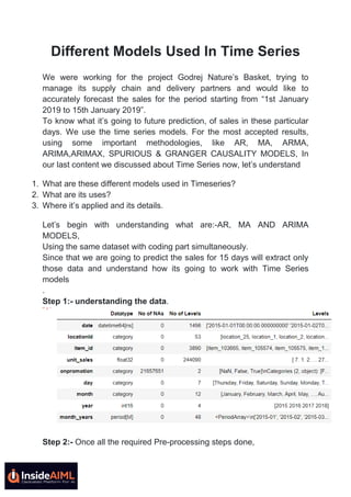
Step 1:- understanding the data.
Step 2:- Once all the required Pre-processing steps done,

2. Step 3:- Explore some Time series plots.
Since that we are going to explore the sales, lets verify with basic of
Timeseries steps those are Residual, Seasonal, Trend of the selected
dataset.
Key Observation:-
1. Seasonality looks more like additive seasonality.
2. This is a strong indication of trend over 4 years and seasonality across
months.
3. Clearly there is yearly trend, with monthly seasonality in the data.

3. Issues with Regressing on Time:-
After walking through basic steps, like working with regression model,
since it is easy and more flexible to work with Timeseries models, and
then finding out the error matrices of seasonality & trend, important
observation one should understand that trend required to capture all the
movements of the data, If there is no trend or if seasonality, and
fluctuations are more important than trend, then the coefficients behave
weirdly. To avoid these major issues one has to work with advance
method of regression which deals with capturing all the movements
present in trend.
What is AR (p) models:- Auto Regressive model
The term AR (Auto Regressive) in simple terms refers to working
auto/self-taking help of regression is called auto regressive.
It will help us to predict/to forecast the variable, of interest using linear
regression, which is the combination of the past values of the variable.
Auto regressive is so flexible to use wide range of different time series
patterns.
Time series has got different styles of understanding the concept, but
let’s use the simplest, and more powerful methods in our content.
Where Auto-regressive model of order p
Ŷ t = α + β1 yt-1 + β2 yt-2 +… βp yt-p

4. 1. This above equation describes about calculations for future prediction
using Ŷ which is the predicted value of y.
2. We find the best value of parameters (β1 , β2,…) that minimize the
errors in forecast of Ŷ t
3. The order of the model p is determined based on the number, beyond
which PACF terms are zero.
4. We normally restrict autoregressive models to stationary data, in which
case some constraints on the values of the parameters are required.
Drawbacks of AR model:-
Where the Timeseries was created out of integration, which although
doesn’t get stationaries even after we difference it, which leads to
quadratic differencing with second differencing, which is called
(Integrated of order II). Which leads to capturing data in all the lags.
Moving Average or MA(q) models:
This method works with two different measures which considers the past
error metrics, captures the regression of order of two coefficients. Where
the largest non-zero terms speaks about the terms required to consider.
Model attempts to predict future values using past error in predictions,Ʃ1
= Ŷ1 — Y1
1. So MA(2) model is Where,
Ŷ t=µ+ϕ1Ʃt-1+ ϕ2Ʃt-2
Where µ, is the average value of the time series, it is the average value
of the time series
• Again, the parameters (ϕ1 ,ϕ2 ) are determined so that prediction error
is minimized.
• The number of terms, q, is determined from the ACF plot. Its the
maximum lag beyond which the ACF is 0

5. ARMA(p,q) model:-
which is called ―Autoregressive moving average model‖, which is the
combination of both the models which takes two hypermeter, So a
ARMA(2,1) model is which takes the two previous values of AR values
and one error term for the regression. also requires two parameters with
one coefficient.
Ŷ t = α + β1 yt-1 + β2 yt-2+ ϕ1Ʃt-1
ARIMA(p,d,q) Models:-
Which is called ―An autoregressive integrated moving average ―which is
mostly used as an statistical tool, for the timeseries for better
understanding of the data.
Where following are the different parameters used in ARIMA.
• p is the number of autoregressive terms, (a linear regression of the
current value of the series against one or more prior values of the
series.) — Maximum lag beyond which PACF is 0.
• d is the number of non-seasonal differences, (order of the differencing)
used to make the time series stationary,
1. q is the number of past prediction, error terms used for the future
forecasts

6. Example of ARIMA: - A time series of the numbers of users, connected
to the Internet through a server every minute. or the example of our
sales took place in those 15 days movement is been captured in ARIMA
Model.
Note:-The forecast is plotted in dark blue. The dark grey and light grey
regions represent the 80% and 95% confidence intervals.
Few important points to be noted about model identification about time
series model..
Model Identification:-
Before Automated functions were available, one used to use ACF plots
to determine the best value of (p,d,q) for a given dataset
1. Box–Jenkins Methodology: This method is used for Model identification
and model selection, it make sure variables are stationary. also finds the
difference as necessary to get a constant mean and transformations to
get constant variance. Required to Check for seasonality, which Decays
and spikes at regular intervals in ACF plots.

7. 2. Parameter estimation :
It Compute coefficients that best fit the selected model.
 Model checking:
This helps to Check if residuals are independent of each other and
constant in mean and variance over time (white noise).
•Non-seasonal: ARIMA models are denoted ARIMA(p,d,q)
• Seasonal ARIMA: (SARIMA) models are denoted
ARIMA(p,d,q)(P,D,Q)m, where m refers to the number of periods in each
season and (P,D,Q) refer to the autoregressive, differencing and moving
average terms of the seasonal part of the ARIMA model.

8. Identification Phase Step 1: Plot the data (transform data to stabilize
variance, if required)
Step 2: Plot ACF and PACF to get preliminary understanding of the
processes involved.(The suspension bridge pattern in ACF (also,
positive and negative spikes in PACF) suggests non-stationarity and
strong seasonality.)
Step 3: Perform a non-seasonal difference. We are getting read to build
an ARIMA(x,1,y) model
Step 4: Check ACF and PACF of differenced data to explore remaining
dependencies.(The differenced series looks somewhat stationary but
has strong seasonal lags.)
Step 5: Perform seasonal differencing (t0 -t12, t1 -t13, etc.) on the
original time series to get seasonal stationarity. This is the same as an
ARIMA(p,0,q) (x,1,y) 12 model.
Step 6: Check ACF and PACF of seasonally differenced data to explore
remaining dependencies and identify model(s). Strong positive
autocorrelation indicates need for either an AR term or a non-seasonal
differencing

9. Step 7: Perform a non-seasonal differencing on seasonally differenced
data. This is like an ARIMA (p,1,q) (x,1,y) 12 model.
Step 8: Check ACF and PACF to explore remaining dependencies.: This
indicates an ARIMA(1,1,1)(0,1,1)12 model. As the significant lag at
seasonal period is negative, include a Seasonal MA(1) term.
Step 9: Calculate parameters using the identified model(s). Use AIC to
pick the best model.
Evaluation Phase Step 10: Check ACF and PACF of the residuals to
evaluate model. The residuals indicate white noise. Indicates a good
model that can be used for forecasting.
Evaluation Phase Step 10: The residuals indicate white noise. Can be
checked using Ljung-Box test.
Important note: For non-seasonal time series, use h = min(10, n/5) For
seasonal time series, use h = min(2m, n/5), where m is the seasonal
period
h is the maximum lag being considered
n is the # of observations (length of the time series)
rk is the autocorrelation
If residuals are white noise (purely random),then Q has a Chi-Square
distribution with h-p degrees of freedom, where p is the number of
parameters estimated in the model. The residuals indicate white noise.
Can be checked using Ljung-Box test.
Null hypothesis:-Residuals are random
Large p-value indicates, null hypothesis can be accepted.
Model Selection:-
• The number of parameters (p,d,q) needed to fit, depends on the
dataset.
• There are techniques that automate model selection.
• auto.Arima command in R picks the best p,d & q parameters for
ARIMA(p,d,q)
―Prediction is very difficult, especially if it’s about the future.‖ — Niels
Bohr,

10. ARIMAX:-
An ARIMAX (ARIMA with exogenous variables) model is simply a
multiple regression with AR and/or MA terms.
when and why arimax is used lets understand with below live examples
1. It is used for where daily data is provided, & to check what should be the
frequency of the time series?
2. If we find any annual spikes in that situation we can start by declaring
the data as a timeseries object with frequency 365.
ARIMAX Approach
1. If the data is not stationary, find out the difference of yt. then apply the
same differencing to all exogenous variables, xt.
2. Build a (multiple) regression model on the stationarized data.
3. Check for Granger-causality. If xt does not Granger-cause yt, then do
not proceed with ARIMAX. It will not do any better than ARIMA.
For example, yt-yt-1= β1(xt-xt-1)+nt

11. where nt are the residuals (white noise; i.e., constant mean and constant
variance). also Check for white noise of residuals, insignificant
exogenous variables,& multicollinearity among exogenous variables,
signs, etc.
A version of ARIMAX is implemented in forecast package and can be
called from the ―auto.arima function‖.
SPURIOUS REGRESSION:-
It is possible to estimate a regression and find a statistically significant
relationship even if none exists. In time series analysis this is actually a
common occurrence when data are not stationary, which converts the
Univar ate to Multivariate data.
So far, we discussed Time Series problems, with involving a single
variable. there are few drawbacks involves with, and that is where
spurious regression helps to resolve the issue with.
These are few situations where spurious, work better than regression
models.
• We may be able to build better models if we have other causal
variables as well.
• Often, people ignore the time-series property of the data and start build
linear regression models in such cases. This could sometimes lead to
misleading results.
• The R2 values could be high, even though the model might not have
any predictive power.
Example:-A recent consulting project…
which is working on predicting different aspects of price of stocks, and
price movement etc. which helps to understand the variables that impact
stock price of a company finds the Possible predictors: like GDP, Oil
Price, Inflation, Commodity Prices.

12. S&P 500 Index GDP
Explanation:-
Look at initial model Date Range: 1950–2017 and this predictions are
been calculated taking some important dimensions from s&p and GDP
when we try executing with R or Python we require basic predictions
which can be performed using simple calculations..

13. Ok then…
where R-squared gave the value of 0.8653, which is the measurement
used to compare the values of previous predicted value.
1. S&P 500 data has a strong trend (non-stationary)
Any other variable with a trend will also show large R2
lets check with some of the Spurious Regressions Some
Examples/used technology.

14. • So, if directly regressing S&P500 with GDP is wrong, what is the right
thing to do?
What is the real goal?
Our intent is to understand how change in GDP affects the S&P
movements.
1. S&P change vs GDP change.
2. This is equivalent to stationarizing the data before we do the regression.
GRANGER CAUSALITY:-
Granger causality is a statistical concept of causality that is based on
prediction. According to Granger causality, if a signal X1 ―Granger-
causes‖ (or ―G-causes‖) a signal X2, then past values of X1 should
contain information that helps predict X2 above and beyond the
information contained in past values of X2 alone.

15. Difference between Regression and Causality
1. Linear regression detects the presence of correlation between change in
x vs change in y.
2. The examples discussed show that high-correlation, does not imply
causation.
3. Sometimes, we want to know if there is a causal relationship.
4. For eg: — Increased endorphins are associated with decreased stress.
Does increase in endorphins actually cause decrease in stress or are
they just correlated?
5. Is there a way to detect causal relationship between two variables? •
Existence of causal relationship would imply better predictive power for
the models.
6. Auto-regressive model of order p (RESTRICTED MODEL, RM)
Ŷ t = α + β1 yt-1 + β2 yt-2 +…+Ɣp yt-p
where p parameters (degrees of freedom) to be estimated
1. The predictor is said to Granger-cause if can be better predicted using
past values of xt.
2. Simple premise: If X causes Y, then X must precede Y.
3. This implies: — Lagged values of X should be significantly related to Y. —
Lagged Values of Y should NOT be significantly related to X
4. Tests the following H0 : xt does not Granger-cause yt i.e
α1=α2=…..αp=0
5. HA : Granger-causes yt, i.e., at least one of the lags of x is significant.
6. Granger Causality is not true causality.
7. It only says that past values of xt can help predict yt better; i.e.,x
precedes y. For example, Diwali fireworks sales precede (i.e., Granger-
cause) Diwali but they do not cause Diwali.
8. Cannot overrule the possibility of a hidden predictor that is causing both
xt and yt.

16. KEY POINTS TO TAKE AWAY
1. Be suspicious of high R 2 in real-life complex problems, especially when
time is a confounding factor. Possible spurious regression.
2. Granger-Causality can help understand which variables have predictive
influence.
3. Granger-causality doesn’t necessarily mean real causality.
4. You must remove autocorrelation (stationarize the data) before testing
for Granger-causality
Finally we learnt all the necessary points which are required to cover in
time series as well as its models.
Thanking you,
Happy Learning.